ScienceDirect
Available online at www.sciencedirect.comAvailable online at www.sciencedirect.com
ScienceDirect
Structural Integrity Procedia 00 (2016) 000–000
www.elsevier.com/locate/procedia
2452-3216 © 2016 The Authors. Published by Elsevier B.V.
Peer-review under responsibility of the Scientific Committee of PCF 2016.
XV Portuguese Conference on Fracture, PCF 2016, 10-12 February 2016, Paço de Arcos, Portugal
Thermo-mechanical modeling of a high pressure turbine blade of an
airplane gas turbine engine
P. Brandão
a, V. Infante
b, A.M. Deus
c*
aDepartment of Mechanical Engineering, Instituto Superior Técnico, Universidade de Lisboa, Av. Rovisco Pais, 1, 1049-001 Lisboa, Portugal
bIDMEC, Department of Mechanical Engineering, Instituto Superior Técnico, Universidade de Lisboa, Av. Rovisco Pais, 1, 1049-001 Lisboa, Portugal
cCeFEMA, Department of Mechanical Engineering, Instituto Superior Técnico, Universidade de Lisboa, Av. Rovisco Pais, 1, 1049-001 Lisboa, Portugal
Abstract
During their operation, modern aircraft engine components are subjected to increasingly demanding operating conditions, especially the high pressure turbine (HPT) blades. Such conditions cause these parts to undergo different types of time-dependent degradation, one of which is creep. A model using the finite element method (FEM) was developed, in order to be able to predict the creep behaviour of HPT blades. Flight data records (FDR) for a specific aircraft, provided by a commercial aviation company, were used to obtain thermal and mechanical data for three different flight cycles. In order to create the 3D model needed for the FEM analysis, a HPT blade scrap was scanned, and its chemical composition and material properties were obtained. The data that was gathered was fed into the FEM model and different simulations were run, first with a simplified 3D rectangular block shape, in order to better establish the model, and then with the real 3D mesh obtained from the blade scrap. The overall expected behaviour in terms of displacement was observed, in particular at the trailing edge of the blade. Therefore such a model can be useful in the goal of predicting turbine blade life, given a set of FDR data.
© 2016 The Authors. Published by Elsevier B.V.
Peer-review under responsibility of the Scientific Committee of PCF 2016.
Keywords: High Pressure Turbine Blade; Creep; Finite Element Method; 3D Model; Simulation.
* Corresponding author. Tel.: +351 218419991.
E-mail address: [email protected]
Procedia Structural Integrity 2 (2016) 1023–1030
Copyright © 2016 The Authors. Published by Elsevier B.V. This is an open access article under the CC BY-NC-ND license (http://creativecommons.org/licenses/by-nc-nd/4.0/).
Peer review under responsibility of the Scientific Committee of ECF21. 10.1016/j.prostr.2016.06.131
10.1016/j.prostr.2016.06.131
ScienceDirect
Structural Integrity Procedia 00 (2016) 000–000www.elsevier.com/locate/procedia
2452-3216 © 2016 The Authors. Published by Elsevier B.V.
Peer-review under responsibility of the Scientific Committee of ECF21.
21st European Conference on Fracture, ECF21, 20-24 June 2016, Catania, Italy
Material Characterization and Numerical Simulation of a Dissimilar
Metal Weld
Szabolcs Szávai
a,*, Zoltán Bézi
b, Peter Rózsahegyi
ca ,b ,c Bay Zoltán Nonprofit Ltd. for Applied Research, Engineering Division, Iglói street 2., Miskolc 3519, Hungary
Abstract
A 3D thermal-mechanical-metallurgical finite element (FE) model has been developed to investigate the microstructure and the distribution of residual stress of a muck-up represents a dissimilar metal weld (DMW) joint of a VVER 440 reactor pressure vessel safety-end nozzle. In order to capture the correct microstructure evolution a number of material properties were required for present simulations. The first task of mechanical characterization was the determination, with accurate experimental devices and its numerical interpretation, of the mechanical properties in terms of stress-strain curve of all DMW constitutive materials: austenitic stainless steel, ferrite steel, heat affected ferrite steel zone and buttering layers properties. For characterization and validation purpose microstructure and hardness map were also evaluated. To get addition information for further investigation, fracture properties for base materials, heat affected ferrite steel zone and buttering layers were also measured. The welding was simulated by the 3D finite element model using temperature and phase dependent material properties. The commercial finite element code was used to obtain the numerical results by implementing the Goldak’s double ellipsoidal shaped weld heat source and combined convection radiation boundary conditions. The results of the simulation provide the size of the HAZ and the volume of the molten zone. The volume fraction of bainite and martensite can be quantified and serves as an additional response that can be used to validate this model with experiments and to predict phase volume fractions under new processing conditions. This paper also presents the results of the through-thickness residual stress distributions on the certain DMW. The results of FE analyses were compared with the experimental measurements in the ferritic steel section of the weld.
© 2016 The Authors. Published by Elsevier B.V.
Peer-review under responsibility of the Scientific Committee of ECF21.
Keywords: FEM, dissimilar metal weld, material characterisation, residual stress;
* Szabolcs Szávai. Tel.: +36-70-205-6455; fax: +36-46-422-786.
E-mail address: [email protected]
Copyright © 2016 The Authors. Published by Elsevier B.V. This is an open access article under the CC BY-NC-ND license (http://creativecommons.org/licenses/by-nc-nd/4.0/).
1.Introduction
DMWs that are in scope of this paper connecting the reactor pressure vessel with the hot-cold leg, and are produced by fusion welding and their structural stability is strongly affected by welding conditions and post weld heat treatment. This type of welding process produces large residual stresses. The value of tensile stress is commonly equal to the yield strength of joint materials. The residual stress of welding can significantly impair the performance and reliability of welded structures. Therefore it is necessary to map and assess the distribution of these residual stresses in welded joints, but advanced numerical investigation is needed that requires detailed input parameters.
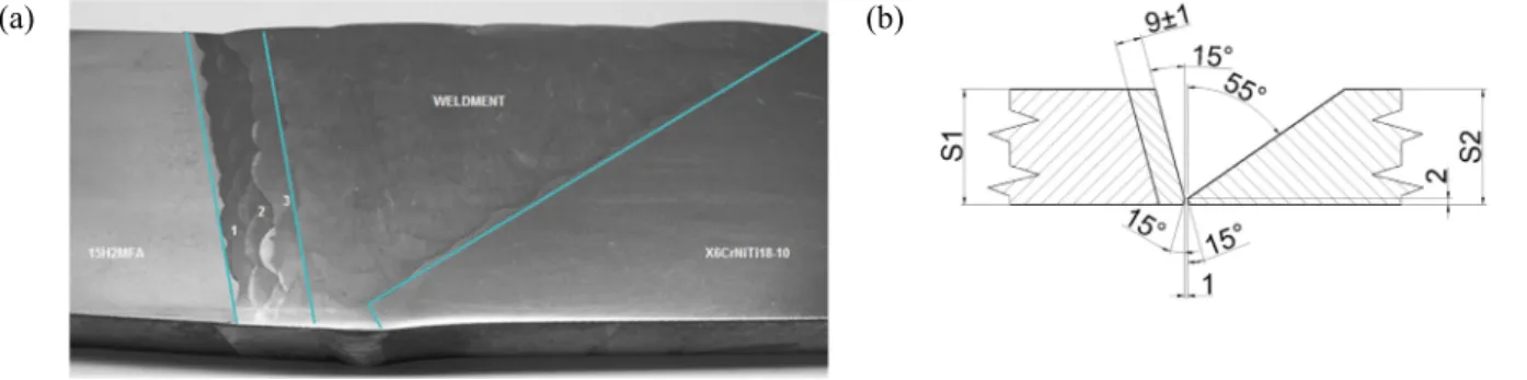
Since the component test cannot be carried out a muck-up was needed was needed for required material characterizations and assessment method verifications. For this purpose an identical muck-up weld has been manufactured. The mock-up reflects the DMW configuration of the WWER-440 reactors connecting the reactor pressure vessel with the hot-cold leg. It involves a bimetallic fusion weld with three buttering layers towards the ferritic side. The goal was to replicate the conditions of a heterogeneous weld in a type VVER 440 reactor pressure vessel RPV nozzle as much as possible with original RPV steel and welding material for buttering layers. It was essential since the interfaces between the RPV steel and the buttering layers are the most sensitive regions. Preparing the mock-up we used the original ferritic steel material and model material for austenitic steel (X6CrNiTi18-10 (1.4541). The original parameters were used for welding and heat treatment. The MU has a thickness of 40 mm. The cushion has two layers. The thickness of the first layer is 3 ± 1 mm and it was welded on by EA-395/9, Ø 4 mm covered stick electrodes. After the first layer was grinded down to meet the thickness criteria, the second layer was welded on, using EA-400/10T Ø 4 mm covered stick electrodes. The total thickness of the layers has to be 9±1 mm (Fig. 1). After cladding, the specimen was heat treated by heating it up to 670°C at a rate of 50°C/h for 16 hours and let it cool down together with the furnace. The welding was performed in two steps and without pre-heating or heat treatment. Originally the root weld was welded from the root side by GTAW method using Sv-04H19N11M3 Ø 1,6 mm electrodes that is no longer commercially available, so a slightly different type of electrode is used, namely Lincoln TIG 316L since its chemical composition is almost the same as the Sv-04H19N11M3. The filling weld and the capping were welded by SAW method using Sv-04H19N11M3 Ø 2 mm electrodes and OF-6 flux in horizontal position (Fig. 1).
(a) (b)
Fig. 1. (a) Macrostructures of butt-welded joint; (b) dimensions of butt-welded joint.
2.Experimental procedure
The first task of mechanical characterization was the determination, with accurate experimental devices and its numerical interpretation, of the mechanical properties in terms of stress-strain curve of all DMW constitutive materials: austenitic stainless steel, ferrite steel, heat affected ferrite steel zone and buttering layers properties. In order to determine the HAZ thickness of 15H2MFA we measured the Vickers hardness (HV1) distribution of the weld. The visualization of these values is on Fig. 2.
Fig. 2. Visualization of the hardness values (HV1) of weld.
The tensile tests were carried out at room temperature and 300 °C. The tensile specimens were worked out parallel with the weld direction. The Fig. 3 shows the positions. The cross section of the specimens is 10x2 mm. For the cutting we used electric cutting machine and drilling machine. The used tensile test machine was an Instron 8850 servohidraulic, biaxial material testing system.
Fig. 3. Tensile test specimen positions (WELD1 includes the buttering layers).
Instrumented hardness testing was planned to use for determining elastic-plastic properties of the different zones of the welded joint of MU3. The comparison of the instrumented hardness test results and tensile test results at room temperature was planned also.
(a) (b)
1.Introduction
DMWs that are in scope of this paper connecting the reactor pressure vessel with the hot-cold leg, and are produced by fusion welding and their structural stability is strongly affected by welding conditions and post weld heat treatment. This type of welding process produces large residual stresses. The value of tensile stress is commonly equal to the yield strength of joint materials. The residual stress of welding can significantly impair the performance and reliability of welded structures. Therefore it is necessary to map and assess the distribution of these residual stresses in welded joints, but advanced numerical investigation is needed that requires detailed input parameters.
Since the component test cannot be carried out a muck-up was needed was needed for required material characterizations and assessment method verifications. For this purpose an identical muck-up weld has been manufactured. The mock-up reflects the DMW configuration of the WWER-440 reactors connecting the reactor pressure vessel with the hot-cold leg. It involves a bimetallic fusion weld with three buttering layers towards the ferritic side. The goal was to replicate the conditions of a heterogeneous weld in a type VVER 440 reactor pressure vessel RPV nozzle as much as possible with original RPV steel and welding material for buttering layers. It was essential since the interfaces between the RPV steel and the buttering layers are the most sensitive regions. Preparing the mock-up we used the original ferritic steel material and model material for austenitic steel (X6CrNiTi18-10 (1.4541). The original parameters were used for welding and heat treatment. The MU has a thickness of 40 mm. The cushion has two layers. The thickness of the first layer is 3 ± 1 mm and it was welded on by EA-395/9, Ø 4 mm covered stick electrodes. After the first layer was grinded down to meet the thickness criteria, the second layer was welded on, using EA-400/10T Ø 4 mm covered stick electrodes. The total thickness of the layers has to be 9±1 mm (Fig. 1). After cladding, the specimen was heat treated by heating it up to 670°C at a rate of 50°C/h for 16 hours and let it cool down together with the furnace. The welding was performed in two steps and without pre-heating or heat treatment. Originally the root weld was welded from the root side by GTAW method using Sv-04H19N11M3 Ø 1,6 mm electrodes that is no longer commercially available, so a slightly different type of electrode is used, namely Lincoln TIG 316L since its chemical composition is almost the same as the Sv-04H19N11M3. The filling weld and the capping were welded by SAW method using Sv-04H19N11M3 Ø 2 mm electrodes and OF-6 flux in horizontal position (Fig. 1).
(a) (b)
Fig. 1. (a) Macrostructures of butt-welded joint; (b) dimensions of butt-welded joint.
2.Experimental procedure
The first task of mechanical characterization was the determination, with accurate experimental devices and its numerical interpretation, of the mechanical properties in terms of stress-strain curve of all DMW constitutive materials: austenitic stainless steel, ferrite steel, heat affected ferrite steel zone and buttering layers properties. In order to determine the HAZ thickness of 15H2MFA we measured the Vickers hardness (HV1) distribution of the weld. The visualization of these values is on Fig. 2.
Fig. 2. Visualization of the hardness values (HV1) of weld.
The tensile tests were carried out at room temperature and 300 °C. The tensile specimens were worked out parallel with the weld direction. The Fig. 3 shows the positions. The cross section of the specimens is 10x2 mm. For the cutting we used electric cutting machine and drilling machine. The used tensile test machine was an Instron 8850 servohidraulic, biaxial material testing system.
Fig. 3. Tensile test specimen positions (WELD1 includes the buttering layers).
Instrumented hardness testing was planned to use for determining elastic-plastic properties of the different zones of the welded joint of MU3. The comparison of the instrumented hardness test results and tensile test results at room temperature was planned also.
(a) (b)
The indentations in the different zone (Weld, Buttering layers, HAZ and ferritic material). The ABIT test results and the tensile test result are in the same diagram on Fig. 4. There are significant differences between the two results. The reason of this may be the different stress state. The strength properties at 300°C can be seen on Fig. 4 as well.
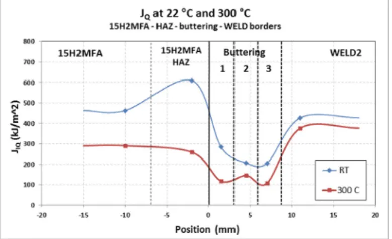
The J-R tests were performed using non side-grooved 10x20 SE(B) specimens at room temperature and at a temperature of +300 °C for ferritic base material, three buffering layers, and for the Ti-stabilised stainless steel base material. Specimens positions are illustrated on Fig. 5. The specimens have surface cracks. The lowest fracture toughness was that of the buffering layers at both temperatures. The values were lowest at +300 °C with estimated ductile tearing onset values JQ of about 100 kJ/m2. The fracture toughness as a function of location and temperature is illustrated in Fig. 6. The precracking and fracture test parameter used are based on ASTM E1820 standard specification. After the fracture tests, the precracked clack length and propagated crack length were measured. The lowest fracture toughness was measured in the buffering layers.
Fig. 5. Cutting plan of the fracture specimens (WELD1: buttering layers, WELD2: austenitic weld).
Fig. 6. The JIQ values measured at room temperature and 300 °C in different layer.
3. 3D finite element modelling
In this paper, a 3D thermal-mechanical-metallurgical finite element (FE) model has been developed to investigate the simulations capability of such kind of joints in real structures.
The welding of DMW mock-up is simulated using three-dimensional (3D) thermo-mechanical and metallurgical finite element model. Work tasks:
Simulate the cladding process
Simulate the heat treatment after the cladding
Simulate the butt-weld process
The FEM pre-processing, calculations and post-processing have been carried out by MSC.Marc and Simufact.welding software based on MSC.Marc code. The thermo-elastic-plastic-metallurgic finite element computational procedure is performed to analyse the welding temperature field and the welding residual stress in DMW mock-up. The thermo-mechanical and metallurgical behaviour is calculated using a coupled formulation.
Fig. 7. FE mesh for DMW
The simulations (in 3D) are done on slightly simplified geometries (Fig. 7). In case of cladding, the welded plate was 200 mm length instead of 780 mm, due to the high costs of computing time and computer resources compare to the case of welding simulation for the full length plate.
One cladding layer is divided to 9 beads along the plate thickness (40 mm). The number of cladding layers was four. In case of welding process, 200 mm length of weld plate is taken account and the total numbers of simulated passes are 39 (Fig. 8). Between welding of the layers ~5 min cooling time is considered, because the interpass cooling temperature is important factor in the final residual stress distribution. Interpass temperature was 250°C in the first cladding layer and it was under 100°C in the other cladding layers and all layer of butt-weld.
(a) (b)
Fig. 8. Welding layers: (a) cladding passes; (b) weld passes.
For DMW simulation, the FE models are created by 8-noded hexagonal elements, number of element is 64120, and number of nodes is 68798. The 15H2MFA plate is modelled as simply supported, during both the cladding sequences and butt-weld sequences. Due to the expected high temperature and stress gradients near the heat source, a relatively fine mesh is used. Element sizes increase progressively with distance from the heat affected zone. In case of butt-weld a relatively coarser mesh is used.
MSC.Marc software uses Goldak’s heat source model for welding simulation. The heat source distribution combines two different ellipses, i.e. one in the front quadrant of the heat source and the other in the rear quadrant. Goldak’s double ellipsoidal shaped weld heat source can be used to specify volume fluxes in 3D as it is presented in Goldak et al. (1984) and MSC.Marc software guide (2013).
MSC.MARC code contains the implementation of material addition or removal technique is very suitable for simulating welding processes Lindgren et al. (1999). The technique requires that the complete model, including all material volume during the whole process, to be defined and meshed in advance. In the deactivated element method,
The indentations in the different zone (Weld, Buttering layers, HAZ and ferritic material). The ABIT test results and the tensile test result are in the same diagram on Fig. 4. There are significant differences between the two results. The reason of this may be the different stress state. The strength properties at 300°C can be seen on Fig. 4 as well.
The J-R tests were performed using non side-grooved 10x20 SE(B) specimens at room temperature and at a temperature of +300 °C for ferritic base material, three buffering layers, and for the Ti-stabilised stainless steel base material. Specimens positions are illustrated on Fig. 5. The specimens have surface cracks. The lowest fracture toughness was that of the buffering layers at both temperatures. The values were lowest at +300 °C with estimated ductile tearing onset values JQ of about 100 kJ/m2. The fracture toughness as a function of location and temperature is illustrated in Fig. 6. The precracking and fracture test parameter used are based on ASTM E1820 standard specification. After the fracture tests, the precracked clack length and propagated crack length were measured. The lowest fracture toughness was measured in the buffering layers.
Fig. 5. Cutting plan of the fracture specimens (WELD1: buttering layers, WELD2: austenitic weld).
Fig. 6. The JIQ values measured at room temperature and 300 °C in different layer.
3. 3D finite element modelling
In this paper, a 3D thermal-mechanical-metallurgical finite element (FE) model has been developed to investigate the simulations capability of such kind of joints in real structures.
The welding of DMW mock-up is simulated using three-dimensional (3D) thermo-mechanical and metallurgical finite element model. Work tasks:
Simulate the cladding process
Simulate the heat treatment after the cladding
Simulate the butt-weld process
The FEM pre-processing, calculations and post-processing have been carried out by MSC.Marc and Simufact.welding software based on MSC.Marc code. The thermo-elastic-plastic-metallurgic finite element computational procedure is performed to analyse the welding temperature field and the welding residual stress in DMW mock-up. The thermo-mechanical and metallurgical behaviour is calculated using a coupled formulation.
Fig. 7. FE mesh for DMW
The simulations (in 3D) are done on slightly simplified geometries (Fig. 7). In case of cladding, the welded plate was 200 mm length instead of 780 mm, due to the high costs of computing time and computer resources compare to the case of welding simulation for the full length plate.
One cladding layer is divided to 9 beads along the plate thickness (40 mm). The number of cladding layers was four. In case of welding process, 200 mm length of weld plate is taken account and the total numbers of simulated passes are 39 (Fig. 8). Between welding of the layers ~5 min cooling time is considered, because the interpass cooling temperature is important factor in the final residual stress distribution. Interpass temperature was 250°C in the first cladding layer and it was under 100°C in the other cladding layers and all layer of butt-weld.
(a) (b)
Fig. 8. Welding layers: (a) cladding passes; (b) weld passes.
For DMW simulation, the FE models are created by 8-noded hexagonal elements, number of element is 64120, and number of nodes is 68798. The 15H2MFA plate is modelled as simply supported, during both the cladding sequences and butt-weld sequences. Due to the expected high temperature and stress gradients near the heat source, a relatively fine mesh is used. Element sizes increase progressively with distance from the heat affected zone. In case of butt-weld a relatively coarser mesh is used.
MSC.Marc software uses Goldak’s heat source model for welding simulation. The heat source distribution combines two different ellipses, i.e. one in the front quadrant of the heat source and the other in the rear quadrant. Goldak’s double ellipsoidal shaped weld heat source can be used to specify volume fluxes in 3D as it is presented in Goldak et al. (1984) and MSC.Marc software guide (2013).
MSC.MARC code contains the implementation of material addition or removal technique is very suitable for simulating welding processes Lindgren et al. (1999). The technique requires that the complete model, including all material volume during the whole process, to be defined and meshed in advance. In the deactivated element method,
filler elements are initially deactivated in the analysis and are not shown on the post file. When the elements are physically created by the moving heat source, they are activated in the model and appear on the post file. Inactive elements have been activated initially to simulate the addition of filler material. The thermal and mechanical activation of the elements are separated. The criterion for thermal activation is that an element should be inside the volume of the heat source. Mechanical activation of an element is achieved when the temperature in the element has dropped below a threshold value. The chosen threshold value is 1800 K. On all free surfaces of all FE-models a convective heat loss with a heat transfer coefficient, h=15W/mK and a radiation heat loss using an emissivity coefficient, ε=0.5 are defined.
Full Newton–Raphson solution technique with direct sparse matrix solver is used for obtaining a solution. During the thermal analysis, the temperature and the temperature-dependent material properties change very rapidly MSC.Marc (2013). Thus, it is believed that a full Newton–Raphson technique using modified material properties gives more accurate results.
4. Material properties
In order to capture the correct microstructure evolution a number of material properties are required for present simulations. The elastic behaviour is modelled using the isotropic Hooke’s rule with temperature-dependent Young’s modulus. The thermal strain is considered in the model using thermal expansion coefficient. The yield criterion is the Von Mises yield surface. In the model, the strain hardening is taken into account using the isotropic Hooke’s law for ferritic steel.
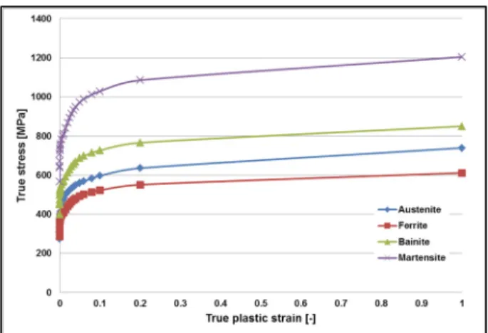
Since the stress-strain curves were available only at room temperature and 300°C and several other imput parameters were required for the simulation, the thermo-metallurgy material properties of 15H2MFA steel were generated with JMatPro software Saunders et al. (2004) based on its chemical composition and corrected to fit the experimental results. Strain hardenings of the phases at room temperature are shown in Fig. 9. Transformation data was calculated using Simufact.premap interface with 8 µm grain size starting at 1200°C.
Fig. 9. Strain hardening of phases for 15H2MFA.
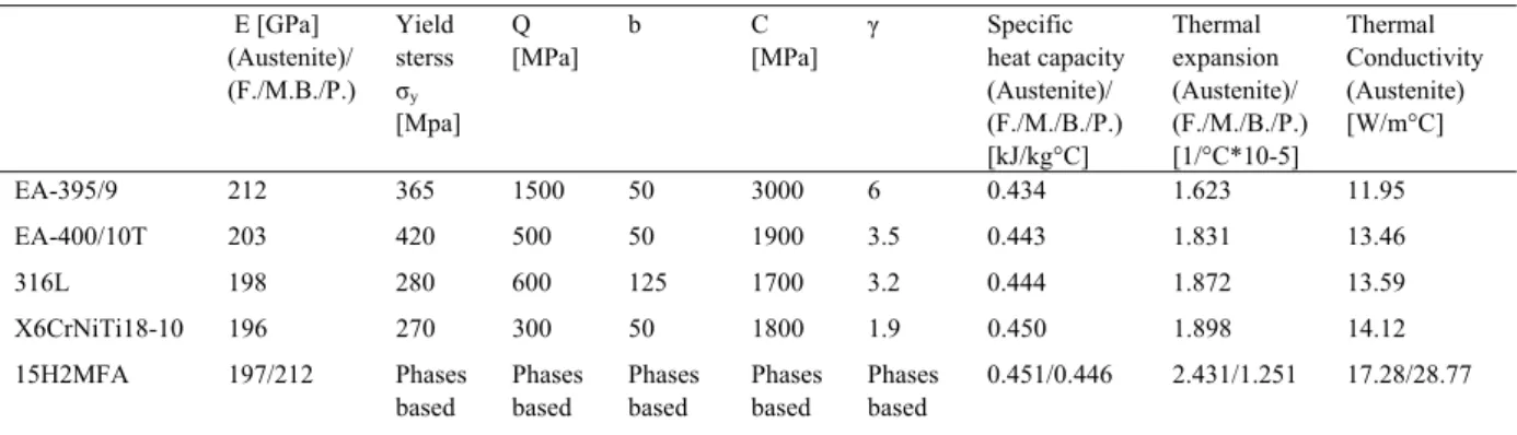
Stainless steel has no solid-state phase transformation during cooling and the heating time is relatively short, it can be expected that the strains due to phase transformation and creep can be neglected in the present simulation. In case of stainless steels, the strain hardening is taken into account using the Chaboche’s combined hardening law Smith et al. (2014). The model in MSC.Marc requires at least five parameters (c, γ, Q, b, σy) which is an acceptable number to be determined from experimental stress vs. strain curves (Table 1). Using these parameters, the model provides an adequate description of the real elastic-plastic material behaviour. Other thermo-mechanical material properties of austenitic steels (Table 1) were generated by JMatPro software. The mixture of the initial microstructure elements in the FE model has to be defined for each material. In case of 15H2MFA 100% bainite and for other materials 100% austenite initial fractions were used Ohms et al. (2015).
Table 1. Thermo- mechanical properties at room temperature. E [GPa] (Austenite)/ (F./M.B./P.) Yield sterss σy [Mpa] Q
[MPa] b C [MPa] γ Specific heat capacity (Austenite)/ (F./M./B./P.) [kJ/kg°C] Thermal expansion (Austenite)/ (F./M./B./P.) [1/°C*10-5] Thermal Conductivity (Austenite) [W/m°C] EA-395/9 212 365 1500 50 3000 6 0.434 1.623 11.95 EA-400/10T 203 420 500 50 1900 3.5 0.443 1.831 13.46 316L 198 280 600 125 1700 3.2 0.444 1.872 13.59 X6CrNiTi18-10 196 270 300 50 1800 1.9 0.450 1.898 14.12 15H2MFA 197/212 Phases
based Phases based Phases based Phases based Phases based 0.451/0.446 2.431/1.251 17.28/28.77
5.Results and discussion
DMW model was validated with available experimental results. A simulation model has been developed and extensive numerical calculations were carried out to find out the residual stress distribution of DMW. The deformed
mesh contour and photograph of DMW section are compared in Fig. 10. The model distortion and the size of the
fusion zone and the heat affected zone (HAZ) are in good agreement with the experimental observations. The results of the simulation provide the size of the HAZ and the volume of the molten zone. The molten zone is the region of the mock-up where the actual weld is formed, while the heat affected zone is the adjacent region where heat may cause solid state phase transformation, but melting does not occur. An additional capability of the model is the ability to predict the volume fraction of various phases.
(a) (b)
Fig. 10. Distortion after welding; (a) deformed shape; (b) distortion at the bottom side.
(a) (b)
filler elements are initially deactivated in the analysis and are not shown on the post file. When the elements are physically created by the moving heat source, they are activated in the model and appear on the post file. Inactive elements have been activated initially to simulate the addition of filler material. The thermal and mechanical activation of the elements are separated. The criterion for thermal activation is that an element should be inside the volume of the heat source. Mechanical activation of an element is achieved when the temperature in the element has dropped below a threshold value. The chosen threshold value is 1800 K. On all free surfaces of all FE-models a convective heat loss with a heat transfer coefficient, h=15W/mK and a radiation heat loss using an emissivity coefficient, ε=0.5 are defined.
Full Newton–Raphson solution technique with direct sparse matrix solver is used for obtaining a solution. During the thermal analysis, the temperature and the temperature-dependent material properties change very rapidly MSC.Marc (2013). Thus, it is believed that a full Newton–Raphson technique using modified material properties gives more accurate results.
4. Material properties
In order to capture the correct microstructure evolution a number of material properties are required for present simulations. The elastic behaviour is modelled using the isotropic Hooke’s rule with temperature-dependent Young’s modulus. The thermal strain is considered in the model using thermal expansion coefficient. The yield criterion is the Von Mises yield surface. In the model, the strain hardening is taken into account using the isotropic Hooke’s law for ferritic steel.
Since the stress-strain curves were available only at room temperature and 300°C and several other imput parameters were required for the simulation, the thermo-metallurgy material properties of 15H2MFA steel were generated with JMatPro software Saunders et al. (2004) based on its chemical composition and corrected to fit the experimental results. Strain hardenings of the phases at room temperature are shown in Fig. 9. Transformation data was calculated using Simufact.premap interface with 8 µm grain size starting at 1200°C.
Fig. 9. Strain hardening of phases for 15H2MFA.
Stainless steel has no solid-state phase transformation during cooling and the heating time is relatively short, it can be expected that the strains due to phase transformation and creep can be neglected in the present simulation. In case of stainless steels, the strain hardening is taken into account using the Chaboche’s combined hardening law Smith et al. (2014). The model in MSC.Marc requires at least five parameters (c, γ, Q, b, σy) which is an acceptable number to be determined from experimental stress vs. strain curves (Table 1). Using these parameters, the model provides an adequate description of the real elastic-plastic material behaviour. Other thermo-mechanical material properties of austenitic steels (Table 1) were generated by JMatPro software. The mixture of the initial microstructure elements in the FE model has to be defined for each material. In case of 15H2MFA 100% bainite and for other materials 100% austenite initial fractions were used Ohms et al. (2015).
Table 1. Thermo- mechanical properties at room temperature. E [GPa] (Austenite)/ (F./M.B./P.) Yield sterss σy [Mpa] Q
[MPa] b C [MPa] γ Specific heat capacity (Austenite)/ (F./M./B./P.) [kJ/kg°C] Thermal expansion (Austenite)/ (F./M./B./P.) [1/°C*10-5] Thermal Conductivity (Austenite) [W/m°C] EA-395/9 212 365 1500 50 3000 6 0.434 1.623 11.95 EA-400/10T 203 420 500 50 1900 3.5 0.443 1.831 13.46 316L 198 280 600 125 1700 3.2 0.444 1.872 13.59 X6CrNiTi18-10 196 270 300 50 1800 1.9 0.450 1.898 14.12 15H2MFA 197/212 Phases
based Phases based Phases based Phases based Phases based 0.451/0.446 2.431/1.251 17.28/28.77
5.Results and discussion
DMW model was validated with available experimental results. A simulation model has been developed and extensive numerical calculations were carried out to find out the residual stress distribution of DMW. The deformed
mesh contour and photograph of DMW section are compared in Fig. 10. The model distortion and the size of the
fusion zone and the heat affected zone (HAZ) are in good agreement with the experimental observations. The results of the simulation provide the size of the HAZ and the volume of the molten zone. The molten zone is the region of the mock-up where the actual weld is formed, while the heat affected zone is the adjacent region where heat may cause solid state phase transformation, but melting does not occur. An additional capability of the model is the ability to predict the volume fraction of various phases.
(a) (b)
Fig. 10. Distortion after welding; (a) deformed shape; (b) distortion at the bottom side.
(a) (b)
The volume fraction of bainite and martensite (Fig. 11) can be quantified and serve as an additional response that can be used to validate this model with experiments and to predict phase volume fractions under new processing conditions. Fig. 12 represents the residual stress distributions of the model after welding. As expected, generally lower stresses in base metal and higher stresses in HAZs as well as welded zones were calculated.
Fig. 12. Residual stress distribution [Pa] after but-weld. 6. Summary
In this study, residual stress prediction was carried out for dissimilar metal welded mock-up. Three-dimensional model was utilized to predict stress fields after welding, especially the longitudinal residual stresses which are in general most harmful to the integrity of the structure among the stress components, in dissimilar steel butt-welded joints between ferritic and austenitic steels which are in essence have different thermal and mechanical properties.
All results are presented considering temperature dependent material properties, phase change, and convection boundary. Also, experimental measurements employing neutron diffraction have been conducted to assess residual stresses within the welded samples. An acceptable agreement has been found between the predicted and the measured data that verifies the validity of the employed model. The simulation results suggest obtaining a highly precise prediction of final residual stress in the joint of the dissimilar metals. Furthermore, considering the important manufacturing processes and developing more reasonable material models are necessary. Both the numerical model and the experiment show that strain hardening consent to the final residual stresses.
7. Acknowledgement
The presented work was carried out as a part of the MULTIMETAL project that has received funding from the European Community’s Seventh Framework Program (FP7/2012- 2015) under grant agreement n◦295968.
References
Goldak, J., Chakravarti, A., Bibby, M., 1984. A new finite element model for welding heat sources model. Metallurgical Transactions B. 15, 299-305.
MSC.Marc 2013.1 Volume A: Theory and User Information
Lindgren, L.-E., Runnemalm, H., Näsström, M., 1999.Simulation of multipass welding of a thick plate. International Journal for Numerical Methods in Engineering 44(9),1301-1316.
Saunders, N., Guo, Z., Li, X., Miodownik, A.P., Schillé, J.P., 2004. The calculation of TTT and CCT diagrams for general steels, Internal report, Sente Software Ltd., U.K..
Smith, M.C., Smith, A.C., Wimpory, R., 2014. A review of the NeT Task Group 1 residual stress measurement and analysis round robin on a single weld bead-on-plate specimen, International Journal of Pressure Vessels and Piping, 93–140.
Ohms, C., Martin, O., Bezi, Z., Beleznai, R., Szavai, Sz., 2015. MULTIMETAL Deliverable D3.10, Residual Stress Measurements of Mockup-3. Technical report, JRC, BZF.


![Fig. 12. Residual stress distribution [Pa] after but-weld.](https://thumb-us.123doks.com/thumbv2/123dok_us/1446131.2693570/8.816.260.560.192.420/fig-residual-stress-distribution-pa-weld.webp)
