University of Arkansas, Fayetteville
ScholarWorks@UARK
Theses and Dissertations5-2018
Parameterizing and Aggregating Activation
Functions in Deep Neural Networks
Luke Benjamin Godfrey
University of Arkansas, Fayetteville
Follow this and additional works at:http://scholarworks.uark.edu/etd Part of theArtificial Intelligence and Robotics Commons
This Dissertation is brought to you for free and open access by ScholarWorks@UARK. It has been accepted for inclusion in Theses and Dissertations by an authorized administrator of ScholarWorks@UARK. For more information, please [email protected], [email protected].
Recommended Citation
Godfrey, Luke Benjamin, "Parameterizing and Aggregating Activation Functions in Deep Neural Networks" (2018).Theses and
Dissertations. 2655.
Parameterizing and Aggregating
Activation Functions in Deep Neural Networks
A dissertation submitted in partial fulfillment of the requirements for the degree of Doctor of Philosophy in Computer Science
by
Luke B. Godfrey University of Arkansas
Bachelor of Science in Computer Science, 2014 University of Arkansas
Master of Science in Computer Science, 2015
May 2018 University of Arkansas
This dissertation is approved for recommendation to the Graduate Council.
——————————————————– Dr. Michael S. Gashler Dissertation Director ——————————————————– Dr. Wing Ning Li Committee Member ——————————————————– Dr. Xintao Wu Committee Member ——————————————————– Dr. Giovanni Petris Committee Member
Abstract
The nonlinear activation functions applied by each neuron in a neural network are essential for making neural networks powerful representational models. If these are omitted, even deep neural networks reduce to simple linear regression due to the fact that a linear combi-nation of linear combicombi-nations is still a linear combicombi-nation. In much of the existing literature on neural networks, just one or two activation functions are selected for the entire network, even though the use of heterogenous activation functions has been shown to produce su-perior results in some cases. Even less often employed are activation functions that can adapt their nonlinearities as network parameters along with standard weights and biases. This dissertation presents a collection of papers that advance the state of heterogenous and parameterized activation functions. Contributions of this dissertation include
• three novel parametric activation functions and applications of each,
• a study evaluating the utility of the parameters in parametric activation functions,
• an aggregated activation approach to modeling time-series data as an alternative to
recurrent neural networks, and
• an improvement upon existing work that aggregates neuron inputs using product
Acknowledgements
I thank Dr. Michael Gashler for his mentorship. He introduced me to the fascinating world of machine learning, a subject about which I have become very passionate under his direction. His time and guidance has been indispensible to my graduate career, and his imagination is truly inspiring. Dr. Gashler made the daunting task of composing a dissertation enjoyable and rewarding, and for that I owe him a great deal of thanks.
I thank my family for all the encouragement, prayer, and love through which they kept me going. I thank my parents for their motivation, support, and example, who often reminded me that God is always in control.
I especially thank my dear wife, Rebekah, who has taken wonderful care of me, staying up late with me on many occasions and being exceptionally patient with her grumpy, sleep-deprived husband. Her love kept me sane and gave me a reason to continue, even when I felt I would never be able to finish this work.
Finally, I thank my great God and Savior, Jesus Christ, without whom none of this would have been possible. The more I study artificial intelligence, the more in awe I am of the one who invented the mind.
Dedication
Contents
I INTRODUCTION 1
1 Deep Neural Networks 2
2 Activation Functions 4
3 Statement and Summary of Contributions 6
3.1 Dissertation Organization . . . 8
II CONTRIBUTIONS 9 4 A Continuum Among Logarithmic, Linear, and Exponential Func-tions, and Its Potential to Improve Generalization in Neural Networks 10 4.1 Introduction . . . 10 4.2 Derivation . . . 11 4.3 Analysis . . . 13 4.4 Inner product . . . 14 4.5 Distance . . . 16 4.6 Polynomials . . . 17
4.7 Radial basis function networks . . . 18
4.8 Fourier networks . . . 18
4.9 Proposed architecture . . . 19
4.10 Conclusion . . . 21
5 A Parameterized Activation Function for Learning Fuzzy Logic Op-erations in Deep Neural Networks 22 5.1 Introduction . . . 22
5.2 Related Work . . . 23
5.3 Approach . . . 25
5.4 Learning Simple Logic Operations . . . 28
5.5 Learning Complex Logic Expressions . . . 30
5.6 Validation . . . 33
5.7 Conclusion . . . 36
6 Neural Decomposition of Time-Series Data 37 6.1 Introduction . . . 37
6.2 Related Work . . . 39
6.2.1 Models for Time-Series Prediction . . . 39
6.2.2 Harmonic Analysis . . . 41
6.3 High Level Approach . . . 45
6.3.1 Algorithm Description . . . 45
6.3.2 Toy Problem for Justification . . . 49
6.3.3 Toy Problem Analysis . . . 51
6.3.4 Chaotic Series . . . 54 6.4 Implementation Details . . . 56 6.4.1 Topology . . . 57 6.4.2 Weight Initialization . . . 57 6.4.3 Input Preprocessing . . . 58 6.4.4 Regularization . . . 59 6.5 Validation . . . 60 6.6 Conclusion . . . 65
7 Leveraging Product as an Activation Function 68 7.1 Introduction . . . 68
7.2 Related Work . . . 69
7.2.1 Product Unit Neural Networks . . . 69
7.2.2 Gated Units . . . 70
7.2.3 Sum-Product Networks . . . 71
7.3 Approach . . . 71
7.4 Applications . . . 74
7.4.1 Representing Polynomials . . . 74
7.4.2 Generalizing Gated Units . . . 74
7.5 Results . . . 76
7.6 Conclusion . . . 79
8 An Evaluation of Parameterized Activation Functions for Deep Learn-ing 80 8.1 Introduction . . . 80
8.2 Related Work . . . 82
8.2.1 Adaptive Transfer Functions . . . 82
8.2.2 Adaptive Piecewise Linear Units . . . 82
8.2.3 Parametric Rectified Linear Units . . . 83
8.2.4 Parametric Exponential Linear Units . . . 84
8.3 Bendable Linear Units . . . 85
8.4 Experiments . . . 88 8.5 Conclusion . . . 94 III CONCLUSION 95 9 Summary 96 10 Future Work 98 References 99
List of Figures
4.1 A plot of h(β,3,7). When β = 0, it correctly calculates 3 + 7 = 10. When
β = 1, it correctly calculates 3∗7 = 21. . . 13
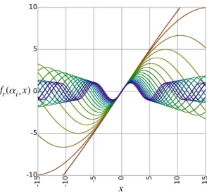
4.2 A plot of f(α, x) for α={−1,−0.9,−0.8,· · · ,0.8,0.9,1.0}from red to purple. 15 4.3 A plot of f(α, x) for x={−5,−4.5,−4,· · · ,4,4.5,5} from red to purple. . . 15
4.4 A neural network implementation of inner product using soft exponential as
an activation function. All of the weights represented with lines in this figure
have a value of 1. All other weights have a value of 0. . . 16
4.5 A neural network implementation of a polynomial,y=a+bx+cx2+dx3. . .,
using soft exponential as an activation function. . . 17
4.6 A neural network implementation of squared distance using soft exponential
as an activation function. To compute Euclidean distance (the square root of
this), only one additional network unit would be required. . . 17
4.7 A plot of the real component of soft exponential over a range of values for αi. 19
4.8 A plot of the imaginary component of soft exponential over a range of values
for αi. . . 21
5.1 Equation 5.2 continuously interpolates among three fuzzy logic operations:
nor, nxor, and and. By allowing biases (true and false) and weights (in
particular, a weight of -1), this equation can also computeidentity,not,or,
xor, and nand. . . 27
5.2 A comparison of Equations 5.1, 5.2, and 5.3 when computing trueαtrue.
Equation 5.1 is smoother, but Equation 5.2 is better suited for use with
gradient-based optimization. . . 29
5.3 A comparison of Equations 5.1, 5.2, and 5.3 when computing trueαfalse.
6.1 Three broad classes of models for time-series forecasting: (A) prediction using a sliding window, (B) recurrent models, and (C) regression-based extrapolation. 40
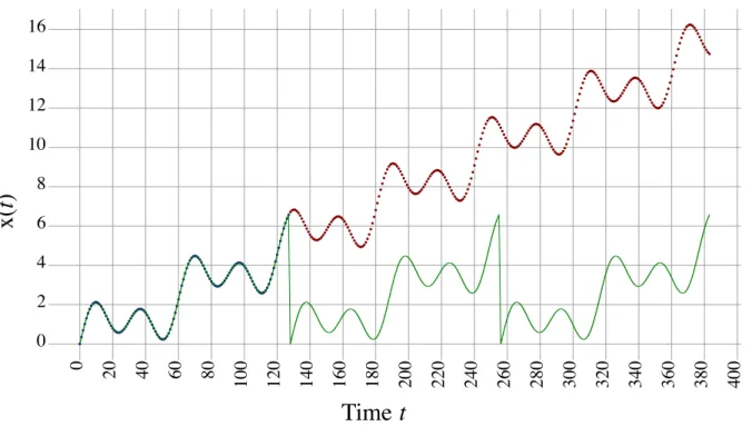
6.2 The predictive model generated by the iDFT for a toy problem with both
periodic and nonperiodic components. Blue dots represent training samples, red dots represent testing samples, and the green line represents the iDFT. Two significant problems limit its ability to generalize: (1) The model repeats, ignoring the linear trend, and (2) The extrapolated predictions misalign with
the phase of the continuing nonlinear trend. . . 43
6.3 A diagram of the neural network model used by Neural Decomposition. For
each of thek sinusoid units,wi are frequencies,φi are phase shifts, andai are
amplitudes, where i∈ {1. . . k}. The augmentation function g(t) is shown as
a single unit, but it may be composed of one or more units with one or more
activation functions. . . 47
6.4 A comparison of Neural Decomposition with two algorithmic variations
show-ing the importance of certain algorithm details. The data used here is the same data used in Figure 6.2. The full ND model, shown in green, fits very closely to the data that was withheld during training. The cyan curve shows predictions made when the basis functions, including sinusoidal frequencies, were frozen during training. Note that the predictions are out-of-phase, indicating that training these components is essential for effective generalization. The orange curve shows predictions made without including any nonperiodic components
among the basis functions, that is, setting the augmentation functiong(t) = 0.
Although the predictions exhibit the correct phase, they fail to fit with the nonperiodic trend. This shows the importance of using heterogeneous basis
6.5 (Top) Frequencies of the basis functions of Neural Decomposition over time. (Bottom) Basis weights (amplitudes) over time on the same problem. Note that ND first tunes the frequencies (Top), then finishes adjusting the
corre-sponding amplitudes for those sinusoids (Bottom) (wA corresponds toφA and
wB corresponds to φB). In most cases, the amplitudes are driven to zero to
form a sparse representation. After the amplitudes reach zero, the frequencies
are no longer modified. . . 50
6.6 Frequency domain representations of the toy problem (amplitude vs frequency).
(Top) Frequencies used by the iDFT. (Bottom) Frequencies used by ND. . . 51
6.7 Neural Decomposition on the Mackey-Glass series. Although it does not
cap-ture all the high-frequency fluctuations in the data, our model predicts the location and height of each peak and valley in the series with a high degree
of accuracy. . . 52
6.8 A comparison of the four best predictive models on the monthly
unemploy-ment rate in the US. Blue points represent training samples from January 1948 to June 1969 and red points represent testing samples from July 1969 to December 1977. SARIMA, shown in magenta, correctly predicted a rise in unemployment but underestimated its magnitude, and did not predict the shape of the data well. ESN, shown in cyan, predicted a reasonable mean, but did not capture the dynamics of the data. LSTM, shown in orange, predicted the first peak in the data, but leveled off to predict only the mean. Only ND, shown in green, successfully predicted both the depth and approximate shape of the surge in unemployment, followed by another surge in unemployment
6.9 A comparison of the four best predictive models on monthly totals of inter-national airline passengers from January 1949 to December 1960 [16]. Blue points represent the 72 training samples from January 1949 to December 1954 and red points represent the 72 testing samples from January 1955 to Decem-ber 1960. SARIMA, shown in magenta, learns the trend and general shape of the data. ESN, shown in cyan, predicts a mean but does not capture the dynamics of the actual data. LSTM, shown in orange, predicts a valley and a peak that did not actually occur, followed by a poor estimation of the mean that suggests that it was unable to learn the seasonality of the data. ND, shown in green, learns the trend, shape, and growth better than the other
compared models. . . 55
6.10 A comparison of the four best predictive models on monthly ozone concentra-tion in downtown Los Angeles from January 1955 to August 1967 [73]. Blue points represent the 152 training samples from January 1955 to December 1963 and red points represent the 44 testing samples from January 1964 to August 1967. The compared models include SARIMA, ESN, LSTM, and ND. All four of these models perform well on this problem. Both LSTM (shown in orange) and ESN (shown in cyan) predict with slightly higher accuracy compared to ND. ND, shown in green, has slightly higher accuracy compared to SARIMA (shown in magenta). ARIMA, SVR, and Gashler and Ashmore’s model all performed poorly on this problem; rather than include them in this
6.11 A comparison of two predictive models on a series of oxygen isotope readings in speleothems in India from 1489 AD to 1839 AD [143]. Blue points repre-sent the 250 training samples from July 1489 to April 1744 and red points represent the 132 testing samples from August 1744 to December 1839. Be-cause this time-series is irregularly sampled (the time step between samples is not constant), only SVR and ND could be applied to it. SVR, shown in orange, does not perform well, but predicts a steep drop in value that does not actually occur in the testing data, followed by a flat line. ND, shown in
green, performs well, capturing the general shape of the testing samples. . . 60
7.1 Test set misclassifications over time of a WPUNN on the MNIST dataset,
fixing s = 1 but varying w. The inverse relationship between accuracy and
window size demonstrates that WPUNNs are sensitive to the hyperparameter
w(window size). Reducing window size solves the major problems associated
with training PUNNs, which validates our primary contribution. . . 73
7.2 A comparison of two neural networks for modeling polynomials. The vertical
axis is error (lower is better) and the horizontal axis is polynomial degree. The green curve is the error rate from a WPUNN and the orange curve is the error rate from a ReLU network. As expected, the WPUNN consistently yields a lower error rate than the ReLU model. The noticable increase in loss
in the WPUNN for d = 9 and d = 10 can be attributed to the depth of the
network being less thanlog(d). . . 75
7.3 Forecasts made by two models on a time-series of Mauna Loa CO2 readings.
Blue points represent training data, red points represent withheld testing data, the green curve represents the forecast by a WPUNN, and the orange curve represents the forecast by a LSTM network. Although the LSTM network yields a more accurate prediction, the WPUNN model is faster and uses a
8.1 A visualization of Bendable Linear Units, varyingα, withβ fixed at 0.9. The
closer α is to 0, the more it is like LReLU [115], and the closer α is to 1, the
more it is like SoftPlus [51]. . . 85
8.2 A visualization of Bendable Linear Units, with α fixed at 0.5. The closer β
is to 0, the more it is like the identity function, and the closer β is to 1, the
steeper the bend. . . 86
8.3 One of the β values from the lowest layer of the WRN-16-4 network using
the BLU-β activation. The initial value, which is about 0.2, is selected from
a uniform random distribution. During the course of training, the network
tunes this value to almost 0, forming a kind of learned residual connection. . 92
8.4 Selected training curves of test set accuaracy on the CIFAR-10 task from our
first experiment. We include curves for BLU, ELU (in orange), PELU (in red), ReLU (in green), and PReLU (in yellow). BLU learns the fastest, but does not converge to as good a final accuracy as PELU and ELU. PELU and ELU achieve approximately the same final result, but PELU converges faster. PReLU, on the other hand, yields significantly better results than ReLU. Thus, for both PELU and PReLU, we observe a benefit to the parameterization. 93
List of Tables
5.1 Average errors of a deep neural network (DNN), an ensemble of ANFIS fuzzy
classifiers (EFC), our model, and the expressions obtained from “snapping” the weights in our network (Snapped) on the validation data for five
classifi-cation problems. Best results arebolded. . . 33
5.2 Logical expressions learned by our model for three of the datasets. These
expressions were formed by “snapping” all parameters of the network to the nearest whole value. Expressions for the other two datasets were omitted for
the sake of brevity. . . 35
6.1 Mean absolute percent error (MAPE) on the validation problems for ARIMA,
SARIMA, SVR, Gashler and Ashmore, ESN, LSTM, and ND. Best result
(smallest error) for each problem is shown in bold. . . 65
6.2 Root mean square error (RMSE) on the validation problems for ARIMA,
SARIMA, SVR, Gashler and Ashmore, ESN, LSTM, and ND. Best result
(smallest error) for each problem is shown in bold. . . 66
8.1 The wide residual network (WRN) topology [172] used in some of our
exper-iments. A WRN has two hyperparameters: d (which controls depth) and k
(which controls width). n, used in the table, is defined as d−64. The final
column, Number, is how many copies of the layer are used in succession. . . 90
8.2 The final CIFAR-10 test set accuracy for each activation/topology pair tested
in our first experiment. The best activation for each topology is shown in bold. Parametric activations tend to achieve higher accuracy than their
8.3 The final CIFAR-10 test set accuracy for each activation using a WRN-16-4 topology in our second experiment, limiting training time to 100 epochs. The parametric activations learn faster than the non-parametric activations. The
best result is shown in bold. . . 92
8.4 The final CIFAR-10 test set accuracy for each activation tested in our third
experiment (using WRN-40-4 with no residual connections). The difference
in accuracy compared with WRN-40-4 with residual connections is reported
in the last column. BLU performed the best in this experiment, both in terms of accuracy and difference in loss. PELU, marked with “x”, diverged during training for several random seeds. ELU achieved good results, despite not being able to approximate the identity function. Though not as good as ELU or BLU, PReLU vastly outperforms ReLU. The best result (highest accuracy
Part I
Chapter 1
Deep Neural Networks
An artificial neural network is a machine learning model that simulates, to the best of our knowledge, how the brain processes electrical signals. In this abstraction, neural networks are made up of neurons (also called nodes) and synapses (also called connections) that link neurons together. A neuron’s output is computed by aggregating its inputs (i.e. as a weighted
sum) and activating the result by applying an activation function such as tanh. One widely
used class of neural networks is multi-layer perceptrons, in which neurons are arranged in layers, with the outputs of one layer being used as inputs to the next. It has been shown that such a neural network with only a single hidden layer (that is, one layer between the input and the output) can serve as a universal function approximator [76]. Neural networks with many hidden layers are called deep neural networks, and depths can range from only six layers [26] to more than 100 [78].
There is a vast body of work involving deep neural networks. Many optimization tech-niques have been studied [70, 157, 95], much work has considered various topologies [118, 148], and several general approaches have been proposed, such as recurrent LSTM networks [75, 49], convolutional networks [102], and reservoir networks [81]. Activation functions, which provide neural networks with the crucial nonlinearities necessary to generalize well,
have also been well-studied [33, 93]. Some of the most popular activation functions aretanh
and rectified linear.
Neural networks are powerful adaptive models with applications in many disciplines. With the backpropagation algorithm, neural networks can be trained in a straightforward manner by gradient-based optimization techniques like stochastic gradient descent and RM-SProp [157]. Several variations of these models are particularly good at certain tasks, such as convolutional neural networks for image classification [102] and LSTM for time-series
analysis [75]. In every neural network, the topology, connections, and nonlinearities play a crucial role to learning.
Chapter 2
Activation Functions
The nonlinear activation functions applied by each neuron in a neural network are critically important for effective learning. In fact, if these are omitted, even deep neural networks reduce to simple linear regression. This is due to the fact that a linear combination of linear combinations is still a linear combination. Thus, activation functions are essential for making neural networks powerful representational models.
For years, sigmoidal activation functions such as tanh have been popular choices [91].
More recently, rectified linear units (ReLUs) have been shown to possess desirable properties [125, 174], as well as a number of variations including leaky ReLUs [115], randomized ReLUs [165], parametric ReLUs [67], and more. Other widely used activations include exponential linear units (ELUs) [27] and scaled ELUs (SELUs) [96].
While these functions perform well empirically, little theoretical basis has been found to justify their extensive use over many other potential functions. In much of the existing literature on neural networks, just one or two activation functions are selected for the entire network, even though the use of heterogenous activation functions has been shown to produce superior results in some cases [159]. Indeed, although using a different activation function for each layer is common, little work has explored mixing multiple activation functions side-by-side within each layer.
Even less often employed are activation functions that can adapt their nonlinearities as network parameters along with standard weights and biases. An adaptable activation func-tion similar to rectified linear but with an arbitrary number of bends was recently proposed and found to achieve state-of-the-art performance on the CIFAR-10 and CIFAR-100 datasets over standard rectified linear networks at the time of its proposal [2]. Parameterized acti-vation functions are not yet widely used, but interest in the topic appears to be building as
Chapter 3
Statement and Summary of Contributions
The aggregation of heterogenous activation functions and the parameterization of activa-tion funcactiva-tions can enable neural networks to model data more quickly and more accurately. Heterogenous activation functions are well-suited for modeling data sampled from the compo-sition of heterogenous signals, while parametric activation functions can be used to promote simpler models to reduce overfitting and generalize more effectively.
Contributions of this dissertation include
• three novel parametric activation functions and applications of each:
– Soft Exponential (SoftExp), which interpolates between logarithm, linear, and
exponential functions,
– the first adaptive transfer function that learns fuzzy logic operations by gradient
descent, and
– Bendable Linear Unit (BLU), which synthesizes properties from parametric
rec-tified linear units (PReLUs), exponential linear units (ELUs), and scaled expo-nential linear units (SELUs) and enables implicit residual connections in deep networks,
• a study evaluating the utility of the parameters in parametric activation functions, in
which we find the following:
– parametric activations achieve (marginally) higher accuracy than their non-parametric
counterparts,
– parametric activations tend to converge more quickly than non-parametric
– parametric activations that can approximate the identity function are more robust than non-parametric activations when removing residual connections,
• an aggregated activation approach to modeling time-series data as an alternative to
recurrent neural networks, which
– empirically shows why the Fourier transform provides a poor initialization point
for generalization and how neural network weights must be tuned to properly decompose a signal into its constituent parts,
– demonstrates the necessity of an augmentation function in Fourier and
Fourier-like neural networks and shows that components must be adjustable during the training process, observing the relationships between weight initialization, input preprocessing, and regularization in this context, and
– unifies these insights to describe a method for time-series forecasting and
demon-strates that this method is effective at generalizing for some real-world datasets,
• an improvement upon existing work that aggregates neuron inputs using product
in-stead of sum, demonstating that
– gradient-based optimization can be used effectively with windowed product units,
– windowed product is as effective as traditional nonlinearities like rectified linear
units (ReLU),
– windowed product unit neural networks can generalize gated units in recurrent
neural networks, and
– our method solves the major problems associated with training product unit
3.1 Dissertation Organization
Chapters 4 through 6 of this dissertation consist of three works that have been published as a result of this dissertation, and Chapters 7 through 8 consist of two works that are currently under consideration for publication. The references for the three published works are listed here, and are ordered according to the chapter in which they appear in this dissertation:
• Luke B Godfrey and Michael S Gashler. A continuum among logarithmic, linear, and
exponential functions, and its potential to improve generalization in neural networks.
InKnowledge Discovery, Knowledge Engineering and Knowledge Management (IC3K),
2015 7th International Joint Conference on, volume 1, pages 481–486. IEEE, 2015
• Luke B Godfrey and Michael S Gashler. A parameterized activation function for
learn-ing fuzzy logic operations in deep neural networks. InSystems, Man, and Cybernetics
(SMC), 2017 IEEE International Conference on. IEEE, 2017
• Luke B Godfrey and Michael S Gashler. Neural decomposition of time-series data for
effective generalization. IEEE transactions on neural networks and learning systems,
2017
It should also be noted that the publication in Chapter 6 builds upon the author’s Masters’ thesis (2015), but is made up of substantially new content not included in that thesis.
Part II
Chapter 4
A Continuum Among Logarithmic, Linear, and Exponential Functions, and Its Potential to Improve Generalization in Neural Networks
Abstract: We present the soft exponential activation function for artificial neural networks
that continuously interpolates between logarithmic, linear, and exponential functions. This activation function is simple, differentiable, and parameterized so that it can be trained as the rest of the network is trained. We hypothesize that soft exponential has the potential to improve neural network learning, as it can exactly calculate many natural operations that typical neural networks can only approximate, including addition, multiplication, inner product, distance, polynomials, and sinusoids.
4.1 Introduction
Each neuron in an artificial neural network applies a non-linear activation function to a weighted sum of its inputs. The activation function serves the important role of enabling the neural network to fit to non-linear curves and surfaces. If omitted, even deep multi-layered neural networks reduce to be functionally equivalent to simple linear regression. Hence, the activation function endows the neural network with its representational power.
One might ask, which activation function is best for neural networks? For years, the
logistic and tanh functions have been popular choices [91]. More recently, rectified linear units have been shown to possess desirable properties [125, 174]. While these functions perform well empirically, little theoretical basis has been found to justify their extensive use over many other potential functions. We present the soft exponential function, a novel activation function with many desirable theoretical properties. It continuously interpolates between logarithmic, linear, and exponential activation functions. It enables neural networks to exactly compute many natural mathematical structures that can only be approximated by
neural networks that use traditional activation functions, including addition, multiplication, exponentiation, dot product, Euclidean and L-norm distance, polynomials, Gaussian radial basis functions, and Fourier neural networks.
The next section derives soft exponential and the remainder of the chapter discusses its desirable properties.
4.2 Derivation
It is well known that multiplication can be implemented by means of addition in logarithmic space. That is,
p∗q =e(logep)+(logeq). (4.1) This property can enable neural networks that use a mixture of logarithmic, linear, and exponential activation functions to exactly perform the basic mathematical operation of multiplication. However, using a mixture of different activation functions in a single neural network adds a significant component of complexity. Specifically, it leaves the user to deter-mine which activation function should be used with each neuron in the network. If a func-tion can be found that continuously generalizes between logarithmic, linear, and exponential functions, then a neural network with a single activation function would be empowered to autonomously learn to add, multiply, exponentiate, and compute the logarithms as needed to accomplish arbitrary tasks. Because these mathematical operations have proven to have significant value in nearly all other areas of science, it is natural to suppose that neural networks should be given the ability to perform the same operations when they attempt to autonomously model various phenomena.
A simple equation that continuously interpolates between linear and exponential func-tions is
g(α, x) = e
αx−1
α +α. (4.2)
Note that limα→0g(α, x) = x, and g(1, x) = ex. This function does not become a
log-arithmic function (i.e. when α = −1), so it does not provide a complete solution to our
objective. However, we can invertg with respect to x to obtain a function that interpolates
between logarithmic and linear functions:
g−1(α, x) = loge(1 +α(x−α))
α . (4.3)
Since g and g−1 are equivalent when α = 0, we can mathematically piece them together
along that edge without breaking continuity. We negateαin the case of the inverse function
and obtain the following continuous piecewise function:
f(α, x) = −loge(1−α(x+α)) α for α <0 x for α= 0 eαx−1 α +α for α >0. (4.4)
Equation 4.4 interpolates between logarithmic, linear, and exponential functions.
Al-though it is spliced together, it is continuous both with respect to α and with respect to
x, and has a number of properties that render it particularly useful as a neural network
activation function. We callf the soft exponential activation function.
We can now address the challenge of creating a continuum of operations between
ad-dition and multiplication. By substituting f into Equation 4.1, we obtain a continuous
generalization between these two operations:
h(β, p, q) =f(β, f(−β, p) +f(−β, q)). (4.5)
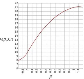
Ifβ = 0, this function addspand q. If β = 1, it multiplies pandq. Figure 4.1 illustrates
-0.1 0 0.1 0.2 0.3 0.4 0.5 0.6 0.7 0.8 0.9 1 1.1 6 7 8 9 10 11 12 13 14 15 16 17 18 19 20 21 22 h(β,3,7) β
Figure 4.1: A plot ofh(β,3,7). When β = 0, it correctly calculates 3 + 7 = 10. Whenβ = 1,
it correctly calculates 3∗7 = 21.
q = 7. At β = 0, it correctly calculates 3 + 7 = 10, and at β = 1, it correctly calculates
3∗7 = 21.
4.3 Analysis
Some of the nice properties of soft exponential include:
• f(−1, x) = loge(x)
• f(0, x) =x
• f(1, x) =ex
• For other values ofα, f(α, x) does something continuous and reasonable.
• The equation is simple, and can be implemented in code with very few operations.
• It appears reasonably smooth when plotted. (See Figures 4.2 and 4.3.)
• For any constant value of α, f(α, x) is monotonic.
• It is continuously differentiable with respect to x,
∂f ∂x = 1 1−α(α+x) for α <0 eαx for α≥0 (4.6) because lim α→0+ ∂f ∂x ≡αlim→0− ∂f ∂x ≡1.
• And it is continuously differentiable with respect to α,
∂f ∂α = loge(1−(α2+αx))− 2α2+αx α2+αx−1 α2 for α <0 x2 2 + 1 for α= 0 α2+(αx−1)eαx+1 α2 for α >0 (4.7) because lim α→0+ ∂f ∂α ≡αlim→0− ∂f ∂α ≡ x2 2 + 1.
• Because it is differentiable, it is possible to train a neural network with soft exponential
using gradient descent. The alpha parameter of the activation function is updated in the same manner as the weights, by stepping in the gradient direction that reduces some objective function.
4.4 Inner product
One operation we might want to generalize is inner product. The inner product is typically implemented as, p·q=p0q0+p1q1+p2q2+. . .. Inner product could be implemented using a 3-layer neural network as depicted in Figure 4.4. This network uses soft exponential for the activation function in each of its units. The first layer computes the logarithm of all
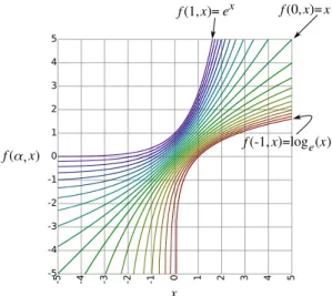
-5 -4 -3 -2 -1 0 1 2 3 4 5 -5 -4 -3 -2 -1 0 1 2 3 4 5 x f(α, ) x x f(1, )= ex x f(-1, )=log ( )ex x f(0, )=x
Figure 4.2: A plot of f(α, x) for α={−1,−0.9,−0.8,· · ·,0.8,0.9,1.0} from red to purple.
-0.5 x f(α, ) α f( ,-5)α f( ,5)α f( ,0)α -1 0 0.5 1 -10 -5 0 5 10
Figure 4.3: A plot of f(α, x) for x={−5,−4.5,−4,· · · ,4,4.5,5} from red to purple.
corresponding elements ofp andq, and exponentiates the result. (All the units in this layer
use α= 1.) The third layer sums all the pair-wise products together. (The unit in this layer
uses α = 0.)
One possible use for this generalization of inner product is to implement a neural network version of matrix factorization, a useful algorithm for recommender systems [98] and missing value imputation for sparse matrix completion [12]. Matrix factorization has also proved to be effective for document clustering [166], text mining and spectral data analysis [7], and molecular pattern discovery [11]. A neural network with our activation function can exactly
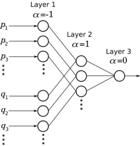
p3 2 p 1 p q3 2 q 1 q α=-1 α=1 α=0 Layer 1 Layer 2 Layer 3
Figure 4.4: A neural network implementation of inner product using soft exponential as an activation function. All of the weights represented with lines in this figure have a value of 1. All other weights have a value of 0.
compute inner product and matrix factorization, and thus it should be able to achieve accuracy at least as good as approaches that do not use neural networks. Because of the flexibility of this generalized approach, it has the potential to outperform direct matrix factorization. For example, in a recommender system, our approach facilitates augmenting user and item profile vectors with static profile vectors for addressing the cold-start problem [98].
4.5 Distance
Suppose we want to compute the distance between two vectors, p and q. This could also
be done with a neural network that uses soft exponential for its activation functions. To do this, we will use the property,
ab =ebloge(a).
Figure 4.6 shows a neural network that computes the squared distance between two vectors. (If you want to take the square root, to make it Euclidean distance, just change the unit in
layer 3 to use α =−1, and add a layer 4 with one unit. This unit would use α = 1, and its
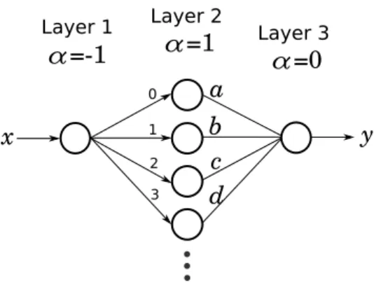
x a α=-1 α=1 Layer 1 Layer 2 2 1 0 α=0 Layer 3 y b c d 3
Figure 4.5: A neural network implementation of a polynomial, y = a+bx+cx2+dx3. . .,
using soft exponential as an activation function.
p3 2 p 1 p q3 2 q 1 q α=-1 α=1 Layer 1 Layer 2 1 1 1 -1 -1 -1 2 2 2 1 α =0 Layer 3 1 1
Figure 4.6: A neural network implementation of squared distance using soft exponential as an activation function. To compute Euclidean distance (the square root of this), only one additional network unit would be required.
4.6 Polynomials
Figure 4.5 shows a neural network that exactly computes an arbitrary polynomial. Mul-tivariate polynomials could also be implemented by simply adding additional units on the input end.
4.7 Radial basis function networks
A gaussian radial basis kernel uses the formula,
e−rs,
whereris a weight that controls the squared radius of the kernel, ands is either the squared
distance between the input vector and the center of the kernel, or the inner product with the input vector. This function is important to a number of classification models, including support vector machines that use a radial basis function and radial basis function networks
[138, 18, 130]. This could be implemented in a network using onlyf as an activation function
by simply adding a single unit withα= 1 to the neural networks in Figures 4.4 or 4.6. The
weight feeding into this unit would be −r. If we added a layer to combine several of these,
we would have a radial basis function network without using any specialized units.
Although it is already well-known that neural networks are universal function approx-imators [29], it is worth noting that soft exponential enables common architectures to be exactly implemented using a neural network with minimal architectural overhead. If a simple model sufficiently models a set of data, it is generally preferable and yields better predictions than an unnecessarily complex one. If these architectures were implemented using a network with a sigmoidal activation function, for example, the resulting models would be very large networks that would probably take more training data to train it to generalize well.
4.8 Fourier networks
Fourier neural networks use a sinusoidal activation function to transform a signal from the time or space domain to the frequency domain in a process similar to the Fourier transform
[141, 154, 182]. If α is allowed to have a complex value, soft exponential can be used as the
activation function in a Fourier neural network. Let αr be the real component of α, and αi
-15 -10 -5 0 5 10 15 -10 -5 0 5 10 x f(α, ) x r i
Figure 4.7: A plot of the real component of soft exponential over a range of values for αi.
is real, and αr = 0. Then the equation for f becomes
f(αi, x) = sin(αix) αi +i αi− cos(αix) + 1 αi . (4.8)
Without these assumptions, the resulting equation contains several additional terms.
Figures 4.7 and 4.8 show the real and imaginary components respectively off over a range of
values for αi. It can be seen in these figures that the imaginary component of α determines
the frequency of the sinusoidal wave. (Although it also affects the amplitude, this is not significant because the outgoing weight can compensate to achieve any desired amplitude).
We have shown that Fourier networks are effective for extrapolating real-world time-series data [44]. Because soft exponential can be logarithmic, exponential, linear, or sinusoidal
when α is allowed to be complex, we can create a Fourier network with only this activation
function and achieve the same level of accuracy for generalization and extrapolation.
4.9 Proposed architecture
We conclude our discussion by describing a deep neural network architecture that could potentially use this novel activation function to autonomously achieve all of these
represen-tational capabilities as needed to address a wide range of challenges. Because complex values
for α cause each unit to output two values, instead of one, it may not be immediately clear
how to apply such a network to arbitrary problems. However, if the α parameter values in
the output layer are constrained to take only real values, then this network will behave like traditional neural networks, mapping from any number of input values to any number of
output values. Allowing hidden units to take on complex values for α should not present
any problems because the additional values may simply be fed into the next layer as if the
preceding layer were twice as big. Hence it should be reasonable to use f as the activation
function for every unit in a deep neural network.
The α parameter for each unit could be initialized to 0 + 0i. This has the very desirable
property of initially causing the entire network to behave like linear regression. As training proceeds, it will take on non-linearities only as necessary to fit the data. All of the weights would be initialized with random values drawn from a normal distribution, then normalized such that the primary eigenvalue is 1. Since all of the activation functions are initially the identity function, the problem of vanishing gradients is initially mitigated, enabling very deep networks to be trained efficiently. This activation function does not impose any particular topology on the rest of the network, so the layers could fully-connected or arranged with sparse connections, such as in convolutional layers.
Likewise, the differentiability of soft exponential facilitates optimization with batch
gra-dient descent, stochastic gragra-dient descent, or many other optimization techniques. α can be
updated along with the weights in the manner of steepest descent. L1 regularization should
be applied to promote sparsity. It can be observed that the various common architectures that we can demonstrated with this activation function use sparse connections. It follows,
therefore, that L1 regularization may be expected to work particularly well with this
acti-vation function. Note that L1 regularization can be applied to the α parameter as well as
the weights of the network. When α is pulled toward zero, the network approaches linear
-15 -10 -5 0 5 10 15 -10 -5 0 5 10 x x fi(αi, )
Figure 4.8: A plot of the imaginary component of soft exponential over a range of values for
αi.
represented by the neural network to straighten out.
4.10 Conclusion
We presented a novel activation function, soft exponential, that continuously generalizes among logarithmic, linear, and exponential functions. This function exhibits many desirable theoretical properties that make it well-suited for use as an activation function with neural networks. Empirical validation of these theoretical properties still needs to be performed as future work. Because of the significant potential that this activation function has to impact the effectiveness of deep neural networks, we are anxious to share these ideas with the broader research community now, instead of waiting for our attempts at achieving validation, so that the community may participate in the process of discovering its potential and limitations.
Chapter 5
A Parameterized Activation Function for Learning Fuzzy Logic Operations in Deep Neural Networks
Abstract: We present a deep learning architecture for learning fuzzy logic expressions. Our
model uses an innovative, parameterized, differentiable activation function that can learn a number of logical operations by gradient descent. This activation function allows a neural network to determine the relationships between its input variables and provides insight into the logical significance of learned network parameters. We provide a theoretical basis for this parameterization and demonstrate its effectiveness and utility by successfully applying our model to five classification problems from the UCI Machine Learning Repository.
5.1 Introduction
Neural networks are powerful adaptive models with applications in many disciplines. With the backpropagation algorithm, neural networks can be trained in a straightforward manner by gradient-based optimization techniques like stochastic gradient descent and RMSProp [157]. Some of these models, such as convolutional neural networks, learn parameters that can be visualized, interpreted, and understood in some cases [173]. Most neural networks, however, are considered black boxes [92, 144] and it is difficult to determine the semantic meanings behind learned weights.
Fuzzy inference systems, built on fuzzy logic, are also powerful models. Unlike neural networks, fuzzy inference systems are straightforward to interpret and often use linguistic values [170]. In fact, these systems are functionally equivalent to a subset of neural networks [84]. Fuzzy inference systems are less general than neural networks, however, and many neural network techniques are not easily translated into the domain of fuzzy logic.
fuzzy inference systems. Adaptive fuzzy systems have been studied for decades [85, 83, 111], and neural fuzzy modeling continues to be an active topic of research [20, 17, 94]. One purpose of combining these techniques is to produce a model with the flexibility and accuracy of black-box neural networks and the interpretability of fuzzy systems.
Although neural fuzzy systems are well-studied, existing approaches primarily focus on
combining specific logical operations in a predefined manner, the most common being an or
of ands [85, 83, 104]. Models that restrict themselves to particular kinds of expressions are
limited in the insights they can offer about given datasets. A system that can adaptively choose from a larger set of logical operations, on the other hand, would be able to provide us with more knowledge about the relationships between its various inputs.
We present a deep learning architecture for learning fuzzy logic expressions by using a novel adaptive transfer function. Our model uses an innovative, parameterized, differen-tiable activation function that can learn a number of logical operations by gradient descent. Parameters learned by our model can be interpreted as fuzzy rules and combined to form complex logic expressions, allowing a glimpse into the knowledge gleaned during the training process. In Section 5.6, we report the results of applying our model to five classification problems taken from the UCI Machine Learning Repository [5]. We find that our model is able to learn complex logical expressions and to achieve accuracy comparable to a standard
deep neural network withtanh activation functions.
5.2 Related Work
Fuzzy logic [97] extends boolean logic into a continuous domain. Typically, false is
repre-sented as0,trueis represented as1, and values in between indicate a corresponding “fuzzy”
degree of uncertainty. A typical set of fuzzy operators that generalize the behavior of boolean logic are:
identity(x) =x not(x) = 1−x or(x, y) = 1−(1−x)·(1−y) xor(x, y) =x+y−2·x·y and(x, y) =x·y nor(x, y) = (1−x)·(1−y) nxor(x, y) = 1−(x+y−2·x·y) nand(x, y) = 1−x·y
One of the most common applications of fuzzy logic is to control systems [105] using a fuzzy inference system [171]. A typical fuzzy logic controller uses Gaussian membership functions to “fuzzify” inputs (which may be linguistic [170]), a set of (fuzzy) logical IF-THEN rules to apply to the fuzzified inputs, and a function that aggregates and “defuzzifies” the result to a crisp value that determines the system’s action [84]. For example, a fuzzy inference
system for an autonomous car might have this inference rule: IF speed limit IS low OR traffic
IS dense THEN speed = slow. In this example,low,dense, andslow are linguistic values that
correspond to functions that map raw sensor inputs to real numbers in the range [0..1] where
0 indicates definitely not in the given set, 1 indicates definitely in the set, and anything else represents how typical the input is for the given set. 100 km/h might be 0.5 in the moderate speed set and 0.8 in the fast speed set.
The combination of fuzzy logic with neural networks has been termed “fuzzy modeling” [85], “neural fuzzy systems” [111], and “adaptive fuzzy systems” [83]. These systems were extensively studied in the 1990s [99, 21, 65, 14, 181, 86], and one of the primary reasons was that the weights and parameters of a neural fuzzy system could be interpreted more meaningfully than in a traditional neural network [28]. More recently, fuzzy neural networks have been applied to tracking control [17] and other nonlinear dynamics [94].
One kind of neural fuzzy system is any neural network that directly models a fuzzy inference system [109, 110, 21]. These models generally have five layers: 1) an input layer,
2) a membership layer to fuzzify input, 3) a rules layer that computes products of the second layers outputs, 4) a normalization layer to defuzzify signals, and 5) a summation layer to produce the output. Inputs and outputs to this kind of system are crisp, and the fuzzy logic takes place in the hidden layers of the network. In 1993, Jang and Sun showed that these neural networks are functionally equivalent to fuzzy inference systems [84]. The learning that occurs in this kind of neural fuzzy system tunes the member functions, adjusting means and standard deviations, in addition to the combination weights in the output layer. The
rules layer in these models is implemented as a product-of-inputs [85], which is a logicaland.
The summation layer performs the logical or, and so most of these models result in a logical
or of ands (or a maxof mins [104]).
Another type of neural fuzzy system is any system that uses both fuzzy logic and neural networks as parts of a whole. Chen et. al recently applied this kind of model to solar radiation forecasting, in which the authors used a fuzzy inference system to combine the predictions three separate neural networks like a weighted ensemble [20]. Other models combine fuzzy systems with genetic algorithms [160] or with a Kalman filter [85]. Still others allow inputs, weights, and outputs to be fuzzy [103]. Kwan and Cai proposed the use of “fuzzy neurons” that combine an aggregation function and an activation function with some number of membership functions [104].
5.3 Approach
We take an approach similar to the common five-layer neural fuzzy system [83], although we use a deeper network. Our model is unique not in its topology in the interpretability of its weights, however, but in the adaptive activation function we use that is able to learn several logical operations. Our activation function is parameterized, continuous, and differentiable, and can therefore be tuned by gradient descent. This has an advantage over existing neural
fuzzy systems because it can model more than just an or of ands, and it has an advantage
set by hand.
The fuzzy logic operators listed in Section 5.2 are elegant because they are simple and continuous. However, the symmetry in these equations is difficult to see because our values
are not centered about the origin. If we linearly remap these operations by defining false
to be-1 instead of 0, they become:
identity(x) =x not(x) =−x or(x, y) =−(x−1)(2y−1) + 1 xor(x, y) =−x·y and(x, y) = (x+1)(2y+1) −1 nor(x, y) = (x−1)(2y−1) −1 nxor(x, y) =x·y nand(x, y) =−(x+1)(2y+1) + 1 Then, if we rewrite them in a consistent form, we obtain:
identity(x) = +(x+0)(1+0)1 −0 not(x) = +(x+0)(1−1+0) −0 or(x, y) =−(x−1)(2y−1) −1 xor(x, y) =−(x+0)(1y+0) −0 and(x, y) = +(x+1)(2y+1) −1 nor(x, y) = +(x−1)(2y−1) −1 nxor(x, y) = +(x+0)(1y+0) −0 nand(x, y) =−(x+1)(2y+1) −1
In this form, it is much more apparent that there is symmetry that can be leveraged to unify these operations into a single more general operation. There are many possible functions that perfectly express all of these fuzzy logic operations. Three representative solutions are given in Equations 5.1, 5.2, and 5.3.
xαy = (x+α)(y+α) α2+ 1 −α 2 (5.1) xαy= (x+α)(y+α) |α|+ 1 − |α| (5.2) xαy = |tt|p|t| − |α| where t = (x+α)(y+α) (5.3)
We can plug any of these functions into our table of logical operations to obtain:
identity(x) =x = true0 x
not(x) =−x = false0 x
or(x, y) =not(x-1y) = false0 (x-1y)
xor(x, y) =not(x0 y) = false0 (x0 y)
and(x, y) =x1y
nor(x, y) =x-1y
nxor(x, y) =x0y
nand(x, y) =not(x1 y) = false0 (x1 y)
Figure 5.3 shows a plot of Equation 5.2 with 5 values for α.
Figure 5.1: Equation 5.2 continuously interpolates among three fuzzy logic operations: nor,
nxor, andand. By allowing biases (trueand false) and weights (in particular, a weight of
5.4 Learning Simple Logic Operations
Since Equations 5.1, 5.2, and 5.3 are continuous and differentiable, gradient-based
optimiza-tion techniques could potentially be used with them to find the values forαthat approximate
the logic represented in a set of training examples.
An important and consideration in using gradient descent with fuzzy logic that does not typically occur in more traditional applications for gradient descent is that each training example only provides information about a subset of the parameter space. For example,
suppose α is initialized to a random value between −1 and 1, and suppose the training
pattern 1α1 = 1 is presented for optimizing the value of α by gradient descent. This
training pattern suggests thatα should not be less than 0, because (1nor 1)6= 1. However,
this training pattern does not suggest anything about what specific valueαshould take≥0,
because (1nxor 1) = 1 and (1 and1) = 1 are both equally true.
Figure 5.4 shows a comparison of Equations 5.1, 5.2, and 5.3 for the case of computing
1α1. If α has a value less than 0, then gradient-based optimization methods will adjust α
by moving it closer to 0 no matter which of these three equations is used. As long as the curve in this region is monotonic, the precise shape is not important because these values
are not defined in boolean logic. However, if Equation 5.1 is used, and αhas a value greater
than 0, then gradient-based optimization methods will move αcloser to 0 or 1, whichever is
closer to the current value ofα. This is incorrect behavior because this training pattern does
not provide any information about whether the logical operation should be more like nxor
or more like and. Since both of these operations are consistent with the training pattern, it
would be arbitrary to bias the model in favor of one over the other. Arbitrary parameter adjustments are likely to fight against subsequent training pattern presentations that may convey valid information for that region of the parameter space, resulting in the model
getting stuck in a local optimum. Equations 5.2 and 5.3 correctly adjust α in all regions of
-1 -0.5 0 0.5 1 -1 0 1 Equation 1 Equation 2 α
nor nxor and 1 α 1
Equation 3
Figure 5.2: A comparison of Equations 5.1, 5.2, and 5.3 when computing trueαtrue.
Equation 5.1 is smoother, but Equation 5.2 is better suited for use with gradient-based optimization. -1 -0.5 0 0.5 1 -1 0 1 α
nor nxor and 1 α -1
Equation 1 Equation 2 Equation 3
Figure 5.3: A comparison of Equations 5.1, 5.2, and 5.3 when computingtrueαfalse. Only
Equation 5.2 is well-suited for use with gradient-based optimization.
As another representative case, consider the training pattern 1−α 1 = 1. Perhaps
coun-terintuitively, this pattern provides no information about any region of the parameter space,
because 1nor−1, 1nxor−1, and 1and−1 all evaluate to −1. Correct behavior, therefore,
should not adjust the value of α, regardless of its current value. Figure 5.4 shows that only
Equation 5.2 exhibits the correct behavior for this case. (This does not imply that such pat-terns should be discarded because in a network containing many fuzzy logic units, different
input values would reach each of the units depending on the currentα values.)
The remaining two cases are both mirror images of these cases, so the same analy-sis applies. It follows that Equation 5.2 can be expected to yield correct behavior with
gradient-based optimization in all cases when training with pure boolean logic. Consistent with this intuition, we found experimentally that Equation 5.2 was always able to learning simple boolean logical expressions, while the other equations sometimes became stuck in
local optima. Therefore, we used Equation 5.2 to implementxαywith the remainder of our
experiments.
At this point, we must note a potential problem with our approach: Equation 5.2 is not a t-norm. A t-norm must be commutative, monotonic, and associative, and the value 1 must be the identity element [61]. Although our equation is commmutative and monotonic, it is
not associative and the value 1 is not neutral for all α. Our work is, therefore, not t-norm
fuzzy logic but belongs instead to a broader class of fuzzy logic. For the purpose of this chapter, we use a relaxed definition of fuzzy logic as being any logic with continuous values
between true and false.
5.5 Learning Complex Logic Expressions
We refer to a layer of network units that implement Equation 5.2 as a Fuzzy layer. Thus,
Equation 5.2 is used as a sort of adaptive transfer function. The only parameters to train
in a fuzzy layer are one α value per each unit. Equations 5.4, 5.5, and 5.6 give the partial
derivatives of Equation 5.2, which are necessary to train such layers with gradient-based optimization methods. ∂α ∂x = y+α |α|+ 1 (5.4) ∂α ∂y = x+α |α|+ 1 (5.5) ∂α ∂α = |a|(x+y)−a(xy+ 1) |a|(|a|+ 1)2 (5.6)
for-ward propagation step that computes predictions with current values, (2) a backpropagation step that computes “blame” terms for each layer in the model, and (3) an update step that refines the parameters of the model. Equation 5.2 is used in the forward propagation step. Equations 5.4 and 5.5 are used in the backpropagation step to assign blame to preceding
layers. Equation 5.6 is used in the update step to refine theα values.
Because Equation 5.6 is not continuous at α = 0, special care must be taken in the
implementation of Fuzzy layers to ensure that they do not become stuck at this point. We
addressed this problem in our implementation by adding the statement “if α < then
α ← −α” to our update step. This small addition enables α to cross over the value 0 in
cases where it would otherwise become stuck. As long as is a small value, this will have
negligible impact on training precision. We used the value = 0.001.
Another challenge that arises in learning fuzzy logic is that Equation 5.2 only accepts two
input values,xandy. One possible solution is to try to generalize the equations in a manner
that can support vectors of arbitrary dimensionality. Equation 5.3 can be generalized in this manner, as given in Equation 5.7.
f(−→x , α) = |tt||t|1/n− |α|
wheret =Qn
i(xi +α)
(5.7)
(In Equation 5.7, f is the fuzzy operator, and n refers to the number of elements in
−
→x.) In higher dimensions, or becomes any, and becomes all, and xor becomes parity.
Unfortunately, Equation 5.3 resists gradient-based optimization, so its generalized version is unlikely to do any better, and Equation 5.2 cannot be generalized in this manner. Further, in applications with many variables, it is often unlikely that all variables will
simultane-ously take the same value, which renders the any and all operations to have very limited
utility. Therefore, a good solution should provide a mechanism to select which values feed into each logical operation. This is also consistent with most real-world uses of boolean logical expressions, and logical expressions involving only two variables at a time are more
likely to be easily comprehensible to humans than logic involving many values. Our
solu-tion to this challenge introduces two addisolu-tional layer types, which we call AllPairings, and
FeatureSelector.
An AllPairings layer accepts n inputs, and outputs all n(n−1)/2 possible unordered
pairings of its input values. In order to facilitate theidentityandnotoperations, we
addi-tionally pair each input value with the bias valuestrueandfalse, which increases the total
number of unordered output pairs ton(n−1)/2+2n. This layer type contains no parameters
to train, so it is straightforward to use in a deep network. During the backpropagation step, the blame term assigned to each input unit is simply the sum of the blame terms for all affect output units.
A FeatureSelector layer is identical to a traditional fully-connected linear layer, except with four minor modifications: (1) No bias weights are used, (2) The weights are initialized with uniform values instead of random values, (3) The weights that feed into each unit are
constrained to have values between -1 and 1, and (4) L1 regularization is applied to the
weights in this layer to gently promote sparse connections in this layer. As it is closely related to a fully-connected layer, it produces a weighted sum of its inputs. This allows the network to learn an interpolation between logical expressions learned in the Fuzzy layers. The outputs of a FeatureSelector layer can be re-mapped between -1 and 1 (i.e. through a membership function) before they are used as input to other layers.
Our topology, given the definitions of these two layer types, is as follows. Given n
continuous input values, we first normalize them between -1 and 1; this can be thought of as a single linear membership function (where 1 is “high” and -1 is “low”). Next, we feed the normalized values into an AllPairings layer. We then feed all combinations of value pairings into a Fuzzy layer, which learns an optimal logical operation for each pair of values. The output of the Fuzzy layer is fed into a FeatureSelector layer to manage dimensionality and to produce the desired number of output values. If a deeper topology is desired, we can feed the output of the FeatureSelector layer into another normalizing layer (i.e. a single membership
Table 5.1: Average errors of a deep neural network (DNN), an ensemble of ANFIS fuzzy classifiers (EFC), our model, and the expressions obtained from “snapping” the weights in our network (Snapped) on the validation data for five classification problems. Best results
are bolded.
Dataset DNN EFC Our Model Snapped
Breast Cancer 3.26% 6.42% 2.77% 2.84%
Diabetes 29.68% 24.51% 22.79% 35.06%
Vehicle 18.01% 50.58% 28.71% 67.84%
Waveform 14.95% - 15.27% 68.43%
Yeast 46.12% 67.37% 49.77% 82.94%
function for each output) and repeat the sequence of AllPairings, Fuzzy, and FeatureSelector layers to an arbitrary depth. If no further depth is needed, we can feed the output of the
final FeatureSelector layer into any kind of output layer; we use amaxlayer for classification.
In our validation, we fix the depth of logic layer to two, resulting in the following final 10-layer deep topology: (1) the input 10-layer (identity), (2) a normalization 10-layer (a single linear membership function), (3) an AllPairings layer, (4) a Fuzzy layer, (5) a FeatureSelector
layer, (6) atanhlayer (a single nonlinear membership function with a new input space), (7)
another AllPairings layer, (8) another Fuzzy layer, (9) another FeatureSelector layer, and
(10) a maxlayer for classification.
5.6 Validation
Our goal in this work is not to surpass the accuracy of existing results or to claim any novelty in learning fuzzy logic rules, but to demonstrate an alternative approach to fuzzy learning using a novel adaptive transfer function. We apply our model to five classification problems taken from the UCI Machine Learning Repository [5], comparing it with a regular
deep neural network (DNN) withtanhactivation functions as well as with ensemble of fuzzy
classifiers (EFC) proposed by Canul-Reich et. al in 2007 [13]. Our results demonstrate that our model meets our goal, adaptively learning complex logic expressions by gradient descent
The five classification problems we used were breast cancer, diabetes, vehicle, waveform, and yeast. Errors yielded by four models are compared in Table 5.1. Across all five problems, we fixed our models parameters to demonstrate robustness. In particular, we set the learning rate to 0.01 and the regularization term to 0.0001. We use a DNN topology with a depth and number of weights similar to our model, but with each layer being fully connected and
all activation functions set totanh.
We also include the results reported by Canul-Reich et. al [13] rather than re-evaluating their method ourselves (which is why there is no result for their model on the waveform problem). Their model is an ANFIS-based ensemble of fuzzy classifiers (labeled EFC in Table 5.1). One of the important observations made by Canul-Reich et. al was that their model performed poorly on datasets with more than six input features (vehicle and yeast).
All of the datasets we use have continuous inputs and discrete class outputs. Breast cancer has 9 inputs and 2-class outputs. Our model outperforms both DNN and EFC in terms of accuracy. Diabetes (Pima) has 8 inputs and 2-class outputs. Again, our model achieves higher accuracy than the compared models.
Vehicle has 18 inputs and 4-class outputs. This is an interesting problem because it has a high number of inputs and more than a binary output. The DNN has significantly lower error than our model, likely due to the difficulties fuzzy systems typically have with larger input spaces. However, our model makes more accurate predictions than EFC, demonstrating that although our model is susceptible to problems with large input spaces, it is more robust than some other fuzzy-based approaches.
Waveform has 40 inputs and 3-class outputs. This is a very large input space, so it is an interesting test for a fuzzy-based system like ours. Our model performed well on this problem, yielding test errors only marginally higher than the DNN. (Canul-Reich et. al did not report results on this problem for EFC).
Yeast has 8 inputs and 10-class outputs. Out of the five datasets we used, this had the highest number of output classes, so the results of this test demonstrate how our model
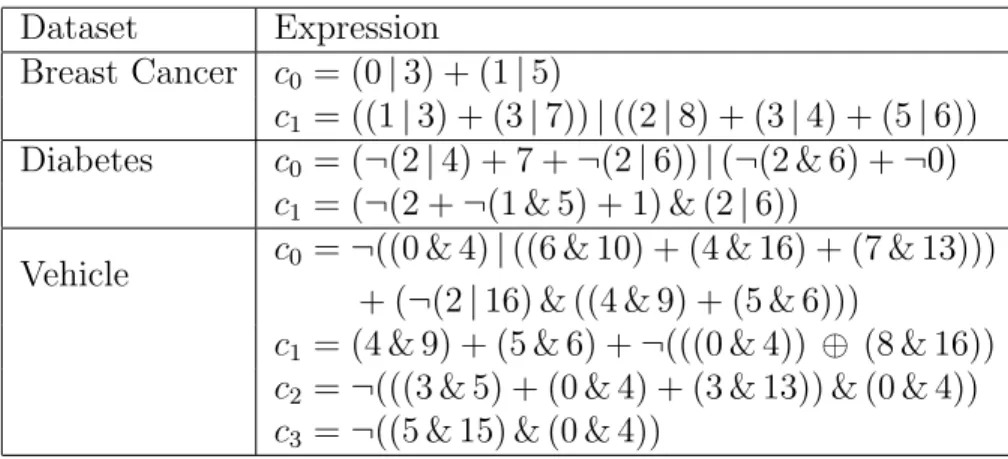
Table 5.2: Logical expressions learned by our model for three of the datasets. These expres-sions were formed by “snapping” all parameters of the network to the nearest whole value. Expressions for the other two datasets were omitted for the sake of brevity.
Dataset Expression
Breast Cancer c0 = (0|3) + (1|5)
c1 = ((1|3) + (3|7))|((2|8) + (3|4) + (5|6)) Diabetes c0 = (¬(2|4) + 7 +¬(2|6))|(¬(2 & 6) +¬0)
c1 = (¬(2 +¬(1 & 5) + 1) & (2|6))
Vehicle c0 =¬((0 & 4)|((6 & 10) + (4 & 16) + (7 & 13))) + (¬(2|16) & ((4 & 9) + (5 & 6)))
c1 = (4 & 9) + (5 & 6) +¬(((0 & 4)) ⊕ (8 & 16))
c2 =¬(((3 & 5) + (0 & 4) + (3 & 13)) & (0 & 4))
c3 =¬((5 & 15) & (0 & 4))
handles many classes. Our model performed nearly as well as the DNN and significantly better than the EFC, demonstrating that it is able to model data with many partitions.
Our model’s weights can be interpreted as complex logical expressions that describe the relationships learned between various inputs. We form these expressions by “snapping” the
α parameters to the nearest whole value (i.e. α = −0.2 snaps to 0 to become nxor) and
“snapping” the weights on the FeatureSelector layer to the nearest whole value (effectively negating expressions with weights near -1 and dropping expressions with weights near 0).
We use n to denote that input n is “high”, ¬ for not, & for and, | for or, and ⊕ for xor.
ci is the output for class i, where the i with maximum ci is the predicted class. Addition
has no equivalent logical operation, so we leave it as a sum indicating the interpolation
between operands. (In the network, the sum is fed through a tanh function to map the
result back into our logical space; this step is omitted in the snapped expressions). The resulting expressions for three of the problems (breast cancer, diabetes, and vehicle) are shown in Table 5.2; expressions for waveform and yeast are omitted from this chapter for brevity. Accuracies of the formed expressions applied to the validation data are reported in the “Snapped” column of Table 5.1.