Representation learning in complex data via pattern discovery

(1)

Representation Learning in Complex

Data via Pattern Discovery

by

Dang Nguyen

(Nguyen Pham Hai Dang)

M.Sc.

Submitted in fulfillment of the requirements for the degree of Doctor of Philosophy

Deakin University

May 2018

(2)

(3)

(4)

Abstract xvii

Acknowledgements xix

Relevant Publications xx

Abbreviations xxii

1 Introduction 1

1.1 Aims and Approaches . . . 2

1.2 Significance and Contributions . . . 4

1.3 Structure of the Thesis . . . 6

2 Related Background 8 2.1 Pattern Discovery . . . 8

2.1.1 Frequent Itemset Mining . . . 8

2.1.1.1 Definitions and problem statement . . . 9

2.1.1.2 Common algorithms . . . 9

2.1.2 Association Rule Mining . . . 14

2.1.3 Sequential Pattern Mining . . . 16

2.1.4 Frequent Subgraph Mining . . . 20

2.1.4.1 Definitions and problem statement . . . 21 iii

(5)

2.2 Representation Learning . . . 23

2.2.1 Feedforward Network and Back-propagation . . . 25

2.2.2 Word2Vec: Learning Word Representation . . . 30

2.2.3 Doc2Vec: Learning Document Representation . . . 34

2.3 Concluding Remarks . . . 36

3 Lattice-based Temporal Association Rule Mining 37 3.1 Introduction . . . 38

3.2 Related Work . . . 40

3.2.1 Data Mining Methods for Cancer Data . . . 40

3.2.2 Temporal Association Rule Mining . . . 41

3.3 Background . . . 43

3.3.1 Clinical Dataset . . . 43

3.3.2 Problem Statement . . . 44

3.4 Framework . . . 47

3.4.1 Building the Lattice Structure of Frequent Codesets . . . 47

3.4.1.1 Lattice structure . . . 47

3.4.1.2 Algorithm . . . 48

3.4.1.3 Complexity analysis . . . 50

3.4.1.4 Illustrative example . . . 50

3.4.2 Mining TARs from the Lattice Structure . . . 50

3.4.2.1 Theorems . . . 51

3.4.2.2 Algorithm . . . 52

3.5 Experiments . . . 55

3.5.1 Discovery of Temporal Toxicity Patterns . . . 55

3.5.1.1 Baseline . . . 56

3.5.1.2 Parameter settings . . . 57

3.5.1.3 Visualization of temporal associations . . . 57

3.5.1.4 Result and discussion . . . 58

3.5.2 Runtime Analysis . . . 63

3.5.2.1 Baseline . . . 63

3.5.2.3 Result and discussion . . . 64 iv

(6)

4 Contrast Set Mining with False Positive Controlling 68

4.1 Introduction . . . 69

4.2 Preliminary Concepts . . . 71

4.2.1 Contrast Set Mining . . . 71

4.2.2 Redundant Contrast Set . . . 74

4.2.3 Problem Statement . . . 75

4.4 CS-Miner: The Proposed Algorithm for Mining Contrast Sets . . . . 77

4.4.1 Finding Large and Non-redundant Contrast Sets . . . 77

4.4.1.1 Tree structure . . . 77

4.4.1.2 Theorem and proposition . . . 78

4.4.1.3 Algorithm . . . 80

4.4.2 Finding Significant Contrast Sets and Controlling False Positives 84 4.4.2.1 Control of false positives . . . 84

4.4.2.2 Algorithm for finding significant contrast sets . . . . 85

4.4.3 Ranking Interesting Contrast Sets . . . 86

4.5 Experiments . . . 87 4.5.1 Experimental Setup . . . 87 4.5.2 Datasets . . . 87 4.5.3 Baselines . . . 88 4.5.4 Runtime Comparison . . . 89 4.5.4.1 Parameter settings . . . 89 4.5.4.2 Evaluation metrics . . . 89

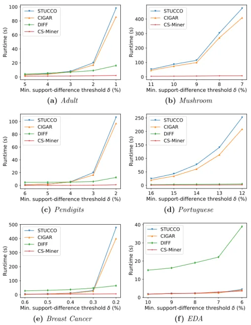
4.5.4.3 Results and discussion . . . 89

4.5.5 Quality Comparison . . . 91

4.5.5.2 Evaluation metrics . . . 91

4.5.6 Classification Comparison . . . 95

4.5.6.1 Parameter settings . . . 95 v

(7)

4.6 Case Study: An Application of CS-Miner to the ED LOS Analysis . . 96

4.6.1 Emergency Department Attendance Dataset . . . 97

4.6.2 Contrast Sets Discovered by CS-Miner . . . 97

4.6.3 Class Association Rules Discovered by CAR-Miner . . . 100

4.6.4 Discussion on the Results Obtained by CS-Miner and CAR-Miner101 4.7 Conclusion . . . 101

5 Learning Transaction Representations via Frequent Itemsets 104 5.1 Introduction . . . 105

5.3 Framework . . . 107

5.3.1 Problem Definition . . . 107

5.3.2 Learning Transaction Embeddings based on Items . . . 108

5.3.3 Learning Transaction Embeddings based on Frequent Itemsets 109 5.3.4 Trans2Vec method for Learning Transaction Embeddings . . . 110

5.3.4.1 Individual-training model to learn transaction em-beddings . . . 110

5.3.4.2 Joint-training model to learn transaction embeddings 111 5.4 Experiments . . . 112

5.4.1 Datasets . . . 113

5.4.2 Baselines . . . 113

5.4.3 Evaluation Metrics . . . 114

5.4.4 Parameter Settings . . . 114

5.4.5 Results and Discussion . . . 115

5.4.6 Parameter Sensitivity . . . 117

5.5 Conclusion . . . 118

6 Learning Sequence Representations via Sequential Patterns 119 6.1 Introduction . . . 119

6.2.1 Sequential Pattern-based Methods for Sequence Representation122 6.2.2 Embedding Methods for Sequence Representation . . . 122

6.3 Framework . . . 123

(8)

6.3.2.2 Sequence embedding learning . . . 126

6.3.3 Sqn2Vec method for Learning Sequence Embeddings . . . 127

6.3.3.1 Sqn2Vec-SEP model to learn sequence embeddings . 128 6.3.3.2 Sqn2Vec-SIM model to learn sequence embeddings . 128 6.4 Experiments . . . 129 6.4.1 Sequence Classification . . . 129 6.4.1.1 Datasets . . . 130 6.4.1.2 Baselines . . . 130 6.4.1.3 Evaluation metrics . . . 131 6.4.1.4 Parameter settings . . . 132

6.4.1.6 Parameter sensitivity . . . 135 6.4.2 Sequence Clustering . . . 135 6.4.2.1 Datasets . . . 135 6.4.2.2 Baselines . . . 136 6.4.2.3 Evaluation metrics . . . 137 6.4.2.4 Parameter settings . . . 137

6.4.2.6 Parameter sensitivity . . . 137

6.4.3 Sequence Visualization . . . 138

7 Learning Graph Representations via Frequent Subgraphs 140 7.1 Introduction . . . 140

7.2 Framework . . . 144

7.2.2 GE-FSG model for Graph Embeddings . . . 144

7.2.2.1 Extract frequent subgraphs . . . 145

7.2.2.2 Associate each graph with a set of FSGs . . . 147

7.2.2.3 Learn graph embeddings . . . 147

7.3 Experiments . . . 148

7.3.1 Graph Classification . . . 149

7.3.1.1 Datasets . . . 149

7.3.1.2 Baselines . . . 150 vii

(9)

7.3.1.6 Parameter sensitivity . . . 153 7.3.2 Graph Clustering . . . 154 7.3.2.1 Datasets . . . 155 7.3.2.2 Baselines . . . 155 7.3.2.3 Evaluation metrics . . . 155 7.3.2.4 Parameter settings . . . 156

7.3.2.6 Parameter sensitivity . . . 157

8 Conclusion and Future Directions 159 8.1 Thesis Contributions . . . 159

8.2 Future Directions . . . 161

A Additional Experiments 163 A.1 LTARM Performance on Large Datasets . . . 163

A.1.1 Datasets . . . 163

A.1.2 Result and Discussion . . . 164

A.2 Diagnosis Code Embedding Learning . . . 165

A.2.1 Problem Statement . . . 166

A.2.2 Word2Vec based Matching (WVM) . . . 166

A.2.3 Experiments . . . 167

A.2.3.1 Dataset . . . 167

A.2.3.2 Baselines . . . 169

A.2.3.3 Readmission matching agreement . . . 169

A.2.3.4 Incidence rate (IR) difference for cancer mortality . . 170

A.2.3.5 Illustration of a pair of matched patients . . . 170

Bibliography 173

(10)

1.1 Thesis structure. . . 7 2.1 A transaction dataset with five transactions (a) and six FIs discovered

from the dataset, with δ= 0.6 (b). . . 10 2.2 A sequential dataset with four sequences (a) and seven SPs discovered

from the dataset, with δ= 0.7 (b). . . 17 2.3 An example graph setG(a) and two subgraphsSG1 andSG2 extracted

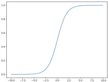
fromG (b). . . 22 2.4 A single unit. . . 25 2.5 The sigmoid function. The x-axis presents uwhile the y-axis presents

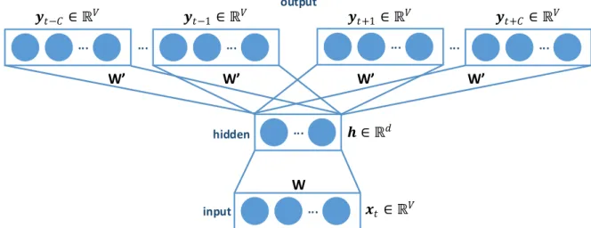
y=σ(u). . . 27 2.6 A multi-layer feedforward network with one hidden layer. . . 28 2.7 Simple version of Skip-gram with only one context word. SG uses the

target word (represented by the vector xt) to predict a context word

(represented by the vector y). . . 31 2.8 Skip-gram model with multiple context words. SG uses the target

word (represented by the vector xt) to predict multiple context words

(represented by the vectors y_t₋_C, ...,y_t₊_C). . . 32

(11)

2.9 Illustration of negative sampling (Gouws, 2016). For every word wt

given its context of 2C previous words wt−C, ..., wt+C, we generate

K negative samples wn from a noise distribution P (we can use a unigram distribution, where a more frequent word is more likely to be selected as a negative sample). Since we need labels to perform our binary classification task, we designate all correct words wt given

their contexts as true labels (i.e., y= 1) and all negative samples wn

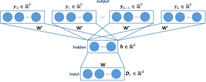
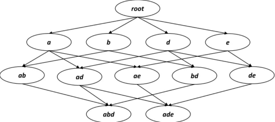
as false labels (i.e.,y= 0). . . 34 2.10 PV-DBOW model. . . 35 3.1 Lattice structure built from the dataset in Table 3.1(a). The name

of a node is also the frequent codeset contained in that node. For example, the nodesa, ab, and abdcontain the frequent codesets {a},

{a, b}, and {a, b, d}, respectively. . . 48 3.2 An example graph for temporal association rule visualization. The

graph represents the rule “1526900: Radiation treatment→(30d) R11: Nausea and E86: Volume depletion”. . . 58 3.3 Network graphs showing toxicities/complications which occur after

one week of radiation treatment. . . 60 3.4 Network graphs showing toxicities/complications which occur after

one month of radiation treatment. . . 61 3.5 Network graphs showing toxicities/complications which occur after

six months of radiation treatment. . . 62 3.6 Number of discovered frequent codesets and rules (a) and the total

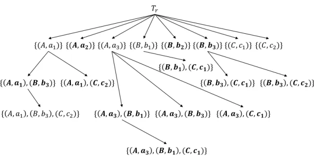
runtimes of Apriori-TARM, FPGrowth-TARM, and ourLTARM (b) on the clinical dataset. . . 65 4.1 Child nodes of the root node. . . 82 4.2 Child nodes of the nodenx ={(A, a1)}. . . 83 4.3 12 large and non-redundant contrast sets remarked in the bold font.

Al-though five contrast sets{(A, a1)},{(A, a3)},{(B, b1)},{(C, c1)}, and

{(C, c2)} are not large, their supmax ≥δ; thus, they are still added to

the tree regarding Theorem4.1. The contrast set{(A, a1),(B, b3),(C, c2)} is large but redundant regarding Theorem 4.2. . . 84 4.4 A plot of the ordered p-values pj of nine contrast sets of size h > 1

and the line with slope j×0₉.05, for the BH method. . . 86

(12)

4.6 Contrast sets discovered by CS-Mineron EDA. . . 98 5.1 Two forms of a transaction: a set of single items and a set of FIs.

Table (a) shows a transaction dataset with five transactions where each of them is a set of items. Table (b) shows six FIs discovered from the dataset (here, δ = 0.6). Table (c) shows each transaction represented by a set of FIs. . . 110 5.2 Individual-training model. Given a transactionTt, we learn the

embed-ding vectorsf1(Tt)andf2(Tt)based on its items and FIs, respectively.

We then take the average of f1(Tt) and f2(Tt) to obtain the final

embedding vectorf(Tt). . . 111

5.3 Joint-training model. Given a transactionTt, we learn the embedding

vector f(Tt)for Tt based on both its items and FIs. . . 112

5.4 The number of FIs discovered from the training set ofSnippets dataset perδ. Theδ value selected via the elbow method is indicated by the red dot. . . 115 5.5 Parameter sensitivity in transaction classification on the Snippets,

Cancer, and Food datasets. The minimum supportδ values selected via the elbow method and used in our experiments are indicated by red markers. . . 117 6.1 Two forms of a sequence: a set of single symbols and a set of SPs.

Table (a) shows a sequential dataset with four sequences where each of them is a set of symbols. Table (b) shows five SPs discovered from the dataset (here,4= 1 andδ = 0.7). Table (c) shows each sequence represented by a set of SPs. . . 126 6.2 Sqn2Vec-SEP model. Given a target sequence St, we learn the

embedding vector f1(St) to predict its belonging symbols and learn

the embedding vectorf2(St) to predict its belonging SPs. We then

take the average off1(St) and f2(St) to obtain the final embedding

vector f(St) for St. . . 128

(13)

6.3 Sqn2Vec-SIMmodel. Given a target sequenceSt,I(St) ={e1, e2, ..., ek}

is the set of symbols contained inSt and F(St) ={X1, X2, ..., Xl} is

the set of SPs contained inSt. We learn the embedding vector f(St)

forSt to predict both its belonging symbols and SPs. . . 129

6.4 The number of SPs discovered from thereuters dataset perδ (here,

4 = 4). The red dot indicates the δ value selected via the elbow method. . . 132 6.5 Parameter sensitivity in sequence classification on five datasetsreuters,

aslbu,aslgt, auslan2, and pioneer. The minimum support thresholds

δ selected via the elbow method and used in our experiments are indicated by red markers. . . 136 6.6 Parameter sensitivity in sequence clustering on two text datasets. . . 139 6.7 Visualization of document embeddings onnews using t-SNE (Maaten

and Hinton, 2008). . . 139 7.1 An example graph setG(a) and two subgraphsSG1 andSG2 extracted

fromG (b). . . 146 7.2 The number of FSGs discovered from the PTC dataset per δ. Theδ

value selected via the elbow method is indicated by the red dot. . . . 152 7.3 Parameter sensitivity in graph classification on PTC, NCI1, D&D,

andIMDB-B datasets. The minimum support δ values selected via the elbow method and used in our experiments are indicated by red markers. . . 154 7.4 Parameter sensitivity in graph clustering on WEBKB and 5NG

datasets. The minimum support δ values selected via the elbow method and used in our experiments are indicated by red markers. . . 157 A.1 The number of discovered frequent itemsets and rules (a) and the

runtimes of Apriori-TARM, FPGrowth-TARM, and ourLTARM (b) on theEDA-small dataset. . . 165 A.2 The number of discovered frequent itemsets and rules (a) and the

runtimes of Apriori-TARM, FPGrowth-TARM, and ourLTARM (b) on theEDA dataset. . . 165 A.3 The number of discovered frequent itemsets and rules (a) and the

runtimes of Apriori-TARM, FPGrowth-TARM, and ourLTARM (b) on theRetail-small dataset. . . 166

(14)

on theRetail dataset. . . 167 A.5 Our Word2Vec based Matching (WVM) method. WVM has two

phases. In phase 1, it adapts the Skip-gram model in Word2Vec (Mikolov et al., 2013) to learn vector representations for ICD codes in EMRs (i.e., the dataset). In phase 2, it selects a set of case patients from the dataset. For each case patientT C, it finds a set of candidate patients ofT C from the dataset, who share several common characteristics withT C. Using the ICD code vectors learned in phase 1, it finds a control patient forT C from the set of candidate patients. 168 A.6 Kalap-Meier curves for three patient groups. In each figure, random

200 case patients are first selected (i.e., the ground truth), and their control patients are then matched by two methods, namelyCSM and our method WVM-Man. In Figure (a), the IR difference between the case patients and the control patients matched byCSM is0.19−0.13 = 0.06 while the IR difference between the case patients and the control patients matched by our WVM-Man is only 0.17−0.13 = 0.04. In Figure (b), the IR differences forCSM and WVM-Man are 0.02 and 0.01, respectively. . . 171 A.7 A randomly drawn case patient and the two control patients matched

by CSM and our WVM-Man. In Figure (a), the case patient consists of the primary diagnosis M17.9 ("Osteoarthritis of knee") and two other conditions: “Essential hypertension” (I10) and “Intraoperative and Postprocedural complications” (I97.8 and Y83.1). In Figure (b),

CSM ignored the order of codes in the coding sequence, and returned a control patient with the primary diagnosis Z50.9 ("Care involving use of rehabilitation procedure"). Its matched control patient also involves “Malignant colon cancer” (C18.0), a condition is not in Figure (a).

In contrast, our WVM-Man returned a control patient matching the primary diagnosis and another major condition “Essential hypertension” (I10), as shown in Figure (c). . . 172

(15)

List of Tables

3.1 An illustration of the clinical dataset. Table (a) shows three patients along with their diagnosis codes. Each diagnosis code in a patient is a type of cancer treatment or a toxicity and it is associated with a time-stamp. Tables (b) and (c) describe the meaning of diagnosis

codes and time-stamps, respectively. . . 44

3.2 Valid TARs extracted from the lattice structure in Figure3.1, with λ= 0.7 and 4=30 days. . . 55

3.3 Runtimes (in second) for mining frequent codesets (MFC) and gen-erating rules (GR) of three methods with differentδ values. A lower runtime means better. Bold font marks the best performance in a column. . . 66

4.1 An example dataset, which contains 10 records, three attribute, and one class attribute. . . 72

4.2 The contingency table for X ={(A, a1)}. . . 74

4.3 Algorithms for CSM: An overview. . . 76

4.4 Characteristics of the experimental datasets. . . 88

4.5 Quality of contrast sets found onAdult by each algorithm. Bold font marks the best performance in each row. . . 92

4.6 Redundancy eliminated by four algorithms on Adult. . . 92

4.7 Quality of contrast sets found onPortuguese by each algorithm. Bold font marks the best performance in each row. . . 93

4.8 Redundancy eliminated by four algorithms on Portuguese. . . 93

4.9 Quality of contrast sets found on Breast Cancer by each algorithm. Bold font marks the best performance in each row. . . 94

(16)

benchmark datasets. Bold font marks the best performance in a column. 96 4.12 Patient and administration characteristics. . . 98 4.13 Contrast set interpretations in the format of “if-then” rules. . . 99 4.14 Quality of contrast sets found on EDA by each algorithm. Bold font

marks the best performance in each row. . . 100 4.15 Redundancy eliminated by four algorithms on EDA. . . 100 4.16 Top 20 class association rules based on confidence discovered by

CAR-Miner onEDA. . . 103 5.1 Statistics of four transaction datasets. . . 113 5.2 Accuracy (AC) and F1-macro (F1) of ourTrans2Vecand six baselines

on four transaction datasets. Bold font marks the best performance in a column. The last row denotes theδ values used by our method for each dataset. . . 116 6.1 Statistics of eight sequential datasets. . . 130 6.2 Accuracy of ourSqn2Vecand 11 baselines on eight sequential datasets.

Bold font marks the best performance in a column. The last row denotes theδ values used by our method for each dataset; they are determined using the elbow method (see Figure6.4). “–” means the accuracy is not available in the original paper. . . 134 6.3 Statistics of two text datasets. . . 136 6.4 MI and NMI scores of our method Sqn2Vec and four baselines on

two text datasets. The MI score is a non-negative value while the NMI score lies in the range[0,1]. Bold font marks the best performance in a column. . . 138 7.1 Statistics of graph datasets, including the number of graphs (|G|), the

average number of nodes (avg. nodes), the average number of edges (avg. edges), the number of graph labels (C), the number of node labels (|LV|), and the number of edge labels (|LE|). “N/A” means

unlabeled nodes/edges. . . 150

(17)

7.2 Classification accuracy (standard deviation) of our methodGE-FSG

and state-of-the-art baselines on benchmark datasets. Bold font marks the best performance in a column. The last row denotes theδ values used by our method for each dataset; these values are determined using the elbow method (see Figure7.2). “-” means the classification accuracy/standard deviation is not available in the original paper. . . 153 7.3 Statistics of text network datasets. The notations are similar to those

in Table7.1. . . 155 7.4 Mutual information (MI) and Normalized mutual information (NMI)

scores of our method GE-FSG and several baselines on two text network datasets. The MI score is a non-negative value while the NMI score lies in the range[0,1]. A higher score means better. Bold font marks the best performance in a column. . . 156 A.1 Statistics of four transaction datasets. . . 164 A.2 Statistics of the cancer dataset. . . 169 A.3 Readmission matching agreement of three baselines and our method

WVM. WVM is tested with three different distances (cosine distance, Euclidean distance, and Manhattan distance). Standard deviation is indicated by Std. A larger agreement means better. Bold font marks the best performance in a column. . . 170 A.4 Incidence rate difference of three baselines and our method WVM.

WVM is tested with three different distances (cosine distance, Eu-clidean distance, and Manhattan distance). Standard deviation is indicated by Std. A smaller IR difference value means better. Bold font marks the best performance in a column. . . 171

(18)

In the decade of big data, data are continuously generated in different forms such as transactions, sequences, and graphs. Representing (orembedding) such complex data as vectors, in a way capturing the hidden structures, semantics, and inter-dependencies, is crucial for effective analysis of the data.

This thesis aims to propose effective and scalable methods for learning meaningful and discriminative representations for transactions, sequences, and graphs.

Our general solution is to leverage meaningful patterns to capture the high-order relations in data, and then learn embeddings based on both atoms and patterns. More specifically, we propose twounsupervised models to learn embeddings fortransactions

via frequent itemsets. Our idea stems from the observation that frequent itemsets are useful for constructing transaction features since they can capture not only the associations among individual items but also the relationships among transactions. Extending our work, we propose twounsupervised models to learn representations for

sequential data. Different from transaction data, sequential data naturally encode the sequential information. Our proposed models capture this information viasequential patterns, and they enforce a gap constraint among symbols in sequences to generate meaningful and discriminative patterns.

In addition to unstructured data (i.e., transactions and sequences), we also research

structured data. We propose anunsupervised model to learn effective embeddings for

graphs. The key success of our model relies on the elegant combination of a recent

neural document embedding model and frequent subgraphs.

Through comprehensive experiments, our proposed models result in superior embed-dings compared with existing state-of-the-art baselines, where they show significant

(19)

improvements in different machine learning tasks such as classification, clustering, and visualization.

Departing from embedding learning models, we also develop algorithms for mining patterns from large datasets. Compared with existing algorithms for pattern discovery, our algorithms are much more efficient in terms of computational cost, where they are 10 times faster than the best competition while they produce high-quality patterns. We demonstrate the practical benefits of our algorithms in the healthcare domain. To the best of our knowledge, this thesis is the first study which combines two impor-tant areas in data mining and machine learning: pattern discovery andrepresentation learning.

(20)

Over the past three years, I have really enjoyed the student life at PRaDA and Deakin University, where I have been very lucky to meet many admirable people. Without them, my PhD study would not have been such an interesting journey. To my principal supervisor – Dr Wei Luo, I am truly grateful for your continuous support, guidance, and encouragement not only in relation to my PhD research but also in my daily life. Your valuable time and effort to guide me in how to write a well-researched academic paper was truly appreciated.

To my associate supervisor – Professor Dinh Phung, I greatly appreciate the way you guided me through difficult problems. Whenever I faced troubles with the research, your valuable advice shed a light and enabled me to continue.

To my associate supervisor – Professor Svetha Venkatesh, I would like to express my deep gratitude to you for your great support. Your positive attitude and endless energy always motivated me to work harder and smarter.

My thanks go to Sunil, Trung, and Truyen for our useful discussions which substan-tially shaped my perspectives. My thanks also go to Bo, Binh, Vu, and Shiva for all your kind support. Especially, my thanks to Tu for your constructive comments on our papers. I learned a lot from them.

To all members of PRaDA, thank you for creating a friendly and enjoyable working environment and for the many social activities we shared together.

To my dear parents, Huong and Dat, and my parents-in-law Hong and Phong, had it not been for your constant support and encouragement, I would not have been able to pursue my dream and follow it to its completion.

Finally, I dedicate this thesis to my beloved wife –Kim Ngan Pham. Your unlimited and unconditional love, support, patience, and sacrifice was my solid and unwavering anchor during my whole PhD journey; I want to call it our PhD journey. I thank you for every moment we have spent together; no matter whether these moments were happy or sad, you have always been there for me.

(21)

Relevant Publications

Part of this thesis has been published or documented elsewhere. The details of these publications are as follows:

Chapter 3:

• Dang Nguyen, Wei Luo, Dinh Phung, Svetha Venkatesh (2015). Understand-ing toxicities and complications of cancer treatment: A data minUnderstand-ing approach.

The Australasian Joint Conference on Artificial Intelligence (AusAI), Canberra, Australia. Springer LNAI, 9457, pp. 431-443.

• Dang Nguyen, Wei Luo, Dinh Phung, Svetha Venkatesh (2018). LTARM: A novel temporal association rule mining method to understand toxicities in a routine cancer treatment. Knowledge-Based Systems (accepted).

Chapter 4:

• Dang Nguyen, Wei Luo, Dinh Phung, Svetha Venkatesh (2016). Excep-tional Contrast Set Mining: Moving Beyond the Deluge of the Obvious. The Australasian Joint Conference on Artificial Intelligence (AusAI), Tasmania, Australia. Springer LNAI, 9992, pp. 455-468.

• Dang Nguyen, Wei Luo, Bay Vo, Dinh Phung, Svetha Venkatesh (2018). Mining Non-redundant Contrast Sets with False Positive Controlling. World Wide Web Journal (under review).

(22)

• Dang Nguyen, Tu Dinh Nguyen, Wei Luo, Svetha Venkatesh (2018). Trans2Vec: Learning Transaction Embedding via Items and Frequent Itemsets. The Pacific-Asia Conference on Knowledge Discovery and Data Mining (PAKDD),

Mel-bourne, Australia. Springer LNAI, 10939, pp. 361-372.

Chapter 6:

• Dang Nguyen, Wei Luo, Tu Dinh Nguyen, Svetha Venkatesh, Dinh Phung (2018). Sqn2Vec: Learning Sequence Representation via Sequential Patterns with a Gap Constraint. The European Conference on Machine Learning and Principles and Practice of Knowledge Discovery in Databases (ECML-PKDD), Dublin, Ireland (accepted, Best Student Machine Leaning Paper Run-ner Up Award).

Chapter 7:

• Dang Nguyen, Wei Luo, Tu Dinh Nguyen, Svetha Venkatesh, Dinh Phung (2018). Learning Graph Representation via Frequent Subgraphs. The SIAM International Conference on Data Mining (SDM), San Diego, USA. SIAM, pp. 306-314.

In addition to the main publications listed above, we adapted the ideas in Chapter 6 to solve the problem of patient similarity matching. The results are reported in

Appendix A and have been published in the following papers:

• Dang Nguyen, Wei Luo, Dinh Phung, Svetha Venkatesh (2016). Control Matching via Discharge Code Sequences. The Conference on Neural Informa-tion Processing Systems (NIPS) Workshop on Machine Learning for Health,

Barcelona, Spain.

• Dang Nguyen, Wei Luo, Svetha Venkatesh, Dinh Phung (2018). Effective Identification of Similar Patients through Sequential Matching over ICD Code Embedding. Journal of Medical Systems, 42(5), Article 94.

(23)

Abbreviations

Abbreviation Meaning

FI Frequent Itemset

SP Sequential Pattern

FSG Frequent Subgraph

TAR Temporal Association Rule

LTARM Lattice-based Temporal Association Rule Mining

CS Contrast Set

CS-Miner Contrast Set Miner

PV-DBOW Paragraph Vector-Distributed Bag-of-Words

LSTM Long Short Term Memory

Bi-LSTM Bidirectional Long Short Term Memory CNN Convolutional Neural Network

GCN Graph Convolutional Network SVM Support Vector Machine EMR Electronic Medical Record

ICD International Classification of Diseases

(24)

Chapter

1

Introduction

“The aim of art is to represent not the outward appearance of things, but their inward significance.”

Aristotle

We are living in the age of digital data, where data are everywhere from large-scale enterprise systems such as supermarkets and banking systems to personal social networks such as Facebook and Twitter. In the past, data were simple and small, and could be easily handled without much effort. However, data nowadays are much more complex in terms of volume and characteristics. For example, every 60 seconds, 1,820 TB of data are created (McKean, 2014) from different sources and in different formats such as transaction data from supermarket and banking/finance systems,

sequential data from instant messages and status updates, graph data from social networks, bio- and chemo-informatics.

The deluge of data makes it impossible to analyze manually. Instead, it is necessary to utilize automated techniques for analysis such as machine learning methods, for example, support vector machine (SVM) (Chang and Lin, 2011) and k-means (Lloyd,

1982). While machine learning methods typically require inputs as fixed-length

feature vectors, many data objects such as word, document, node, and graph do not have such feature vectors by default. Consequently, the application of machine learning methods to such data objects is a challenging problem.

Recently, representation learning methods (aka embedding methods) have emerged as new promising solutions to learn feature vectors (orembedding vectors) for such data

(25)

1.1. Aims and Approaches 2 objects. In particular, representation learning has become a hot trend since 2013 when Mikolov introduced Word2Vec (Mikolov et al.,2013) to learn embedding vectors for words in text. In recent years, embedding methods have been developed to learn

low-dimensional continuous embedding vectors for nodes in networks (Grover and Leskovec,2016), symptoms in healthcare (Nguyen et al.,2018b), values in categorical data (Yoshida et al., 2017), and documents in text (Le and Mikolov, 2014; Chen,

2017).

Although existing embedding methods can learn useful embedding vectors for data objects, which show significant improvements over non-embedding methods in several applications such as document and node classification (Grover and Leskovec, 2016;

Le and Mikolov, 2014; Chen,2017), they still suffer from two important limitations. First, most of them have learned embedding vectors based on atoms in data such as words or nodes; as a result, they are unable to capture the high-order relations in data, e.g., the relations among words (i.e., phrases) or the relations among nodes (i.e., subgraphs). Second, most of them have only focused on the text domain, where they learned embedding vectors for words and documents; meanwhile, embedding methods for other data objects such as transaction, sequence, and graph have not been extensively studied.

To this end, this thesis proposes effective methods for learning representations for non-trivial data objects such as transactions, sequences, and graphs. Our general solution is to leverage interesting and meaningful patterns which can capture the high-order relationships in complex data, and then learn embedding vectors based on both atoms and patterns. Our learned embedding vectors are meaningful, discriminative, and useful in various machine learning tasks, for example, classification, clustering, and visualization.

1.1

Aims and Approaches

In this thesis, we aim to improve the quality of embedding methods in complex data. In particular, our three main objectives are:

• To develop effective models to learn representations for transaction data. We first encode each transaction into two different sets: a set of singleton items and a set offrequent itemsets (FIs) (Fournier-Viger et al., 2017b). We then propose two unsupervised models to learn transaction embeddings: one learns

(26)

embed-dings from these two sets separately, and then takes the average ( individual-training model), and another learns embeddings from these two sets

simultane-ously (joint-training model).

• To develop effective models to learn representations for sequential data. Since

sequential patterns(SPs) (Fradkin and Mörchen,2015) can capture the temporal orders among singleton symbols, we first propose anunsupervised model which learns sequence embeddings based on SPs. Our model is an extension of the PV-DBOW model for learning document embeddings (Le and Mikolov, 2014), where each sequence is treated as a document and SPs are treated as words. To generate meaningful and discriminative SPs, we consider thecontext of each symbol in the sequences. More precisely, we enforce a4-gap constraint among symbols in the sense that the distance between two consecutive symbols must be within a window size 4. We then further propose two unsupervised models to learn sequence embeddings based on both symbols and SPs.

• To develop effective models to learn representations for graph data. Existing methods for learning graph embeddings either ignore the structural information of a graph or only capture the local information of nodes. They also cannot use the available information of edge labels. We propose anunsupervised model to learn graph embeddings based on frequent subgraphs (FSGs) (Yan and Han,

2002). Our model can capture both the semantic of an individual graph and the relationships among graphs, and leverage available edge labels during the learning process. It has three important steps: (1) extracting FSGs from the graph dataset; (2) associating each graph with a set of FSGs; and (3) learning the embedding vector for each graph following the PV-DBOW model (Le and Mikolov,2014).

Departing from embedding models, we also aim to develop efficient algorithms for mining complex patterns in large-scale datasets. In particular, our two subsidiary objectives are:

• To develop an efficient algorithm for temporal association rule mining (TARM). Existing methods for TARM (Nam et al., 2009; Concaro et al., 2011; Nguyen

et al., 2015a) often consist of two phases: (1) mining FIs and (2) generating

temporal association rules (TARs) from discovered FIs. We first construct a lattice structure to discover FIs and encode the paternity relationships among them. We then develop an algorithm to traverse the lattice and generate TARs,

(27)

1.2. Significance and Contributions 4 where we propose two theorems which help to prune invalid candidate rules quickly, thus reducing the number of candidate rules in the search space.

• To develop an efficient algorithm for contrast set mining (CSM). We first adapt the tree structure proposed in class association rule mining (CARM) (Nguyen et al., 2015b,2016c) to search forcontrast sets (CSs) (Bay and Pazzani, 2001). Each node in the tree contains a contrast set with its metadata to easily and quickly compute its support in each group. We then introduce two theorems and one proposition to prune the search space and retain only non-redundant CSs. Finally, we employ the Benjamini and Hochberg’s (BH) method (Benjamini and Hochberg,1995) to control the false positives for multiple testing.

1.2

Significance and Contributions

The significance of this thesis is three-fold: (1) our proposed embedding models provide meaningful representations for transactions, sequences, and graphs, which result in better classification and clustering performance; (2) our proposed mining algorithms offer an efficient solution for data mining practitioners to discover insightful patterns from large-scale data; and (3) our proposed methods can be applied to a wide range of real-world problems including healthcare analysis, business marketing, text mining, action recognition, and bioinformatics. Specifically, our main contributions are:

• An efficient and robust algorithm for TARM (named LTARM). Compared with existing algorithms, our proposed algorithm significantly boosts the mining time, where it achieves a speed which is 5-8 times faster than the baselines. We also use TARs to discover the toxicity progression of cancer treatments. Different from the temporal comorbidity analysis method (Hanauer and

Ra-makrishnan, 2013), our proposed method not only captures the temporal

relations between a cancer treatment and toxicities but also uncovers the co-occurrence of toxicities.

• An efficient and robust algorithm for CSM (named CS-Miner). Compared with three state-of-the-art algorithms for CSM, namely STUCCO (Bay and

Pazzani, 2001), CIGAR (Hilderman and Peckham, 2007), and DIFF (Liu

et al., 2014), our CS-Minersignificantly reduces the mining time while it can produce high-quality CSs. We also introduce a novel application in healthcare

(28)

by applying CS-Miner to the electronic medical records (EMRs) of 399,107 patients to analyze their length of stay (LOS) in the emergency department (ED). We show that CS-Miner can provide comprehensive information on

LOS for different patient populations.

• Two effective unsupervised models (Trans2Vec-IND and Trans2Vec-JOI) for learning transaction embeddings. Since our models learn transaction embed-dings from information of both singleton items and FIs, the embedembed-dings learned are meaningful and discriminative. Our models achieve considerable improve-ments on several benchmark datasets in transaction classification, where they outperform pattern-based baselines by 7-23%. To the best of our knowledge, our models are the first attempt to learn low-dimensional continuous vectors for transactions.

• Two effective unsupervised models (Sqn2Vec-SEP and Sqn2Vec-SIM) for learning sequence embeddings. We first explain why current embedding methods do not work well on sequential data in bioinformatics or navigation systems. We then propose two models for learning sequence embeddings based on singleton symbols and SPs satisfying a gap constraint. We demonstrate the accuracy of our models in sequence classification, where they are significantly better than state-of-the-art unsupervised baselines and highly competitive with state-of-the-artsupervised baselines. We also demonstrate the superior performance of our models in sequence clustering and visualization.

• An effective unsupervised model (GE-FSG) for learning graph embeddings. Our model offers three key advantages: (1) it not only captures the underly-ing semantics within an individual graph but also captures the relationships among graphs; (2) it fully leverages available edge labels during the learning process; and (3) it learns graph representations in a fully unsupervised fashion. Compared with graph kernel-based methods,unsupervised graph embedding methods,supervised graph embedding methods, and graph pattern-based meth-ods, ourGE-FSGachieves remarkable improvements on most datasets in both tasks: graph classification and clustering, where it achieves a 19-24% gain over the closest competition.

(29)

1.3. Structure of the Thesis 6

1.3

Structure of the Thesis

This thesis consists of eight chapters with supplementary sections in the Appendix. The rest of the thesis is organized as follows:

Chapter2: reviews the literature and background relevant to this thesis. This chapter contains two sections. The first section reviews important topics in pattern discovery including frequent itemset mining (FIM), association rule mining (ARM), sequential pattern mining (SPM), and frequent subgraph mining (FSM). The second section focuses on representation learning, where it presents two well-known models for learning word and document embeddings, namely Word2Vec and Doc2Vec, which form the basic framework of our proposed models.

Chapter 3: presents our first contribution to pattern discovery, namely an efficient algorithm for TARM. We first introduce the temporal transaction dataset used in our research and describe the problem statement. We then detail our proposed algorithm, named LTARM, which stands for Lattice-based Temporal Association Rule Mining. Finally, we end this chapter with a comprehensive experiment to qualitatively and quantitatively evaluate the performance of LTARM.

Chapter4: presents our second contribution to pattern discovery, namely an efficient algorithm for CSM. We first provide the preliminary concepts of CSM and discuss three types of redundant CSs. We then introduce our proposed algorithm, named CS-Miner, which stands forContrast Set Miner. We then conduct extensive experiments on six benchmark datasets to validate our proposed algorithm, comparing three state-of-the-art baselines. Finally, we conclude this chapter with an application of

CS-Miner in the healthcare domain.

Chapter 5: introduces our first contribution to representation learning in complex data. More specifically, it proposes a novel method, namedTrans2Vec, for learning transaction embeddings. We first define the problem statement. We then describe the detail of two models in Trans2Vec, which learn embedding vectors for transactions based on information of both singleton items and FIs. Finally, we conduct experiments on real-world transaction datasets to demonstrate the superior performance of our proposed method in transaction classification.

Chapter 6: introduces our second contribution to representation learning in complex data, particularly a novel method, namedSqn2Vec, for learning sequence embed-dings. We first formalize the problem of sequence representation learning. We then

(30)

propose two models inSqn2Vec(Sqn2Vec-SEPandSqn2Vec-SIM), which learn embedding vectors for sequences based on singleton symbols and SPs with a gap con-straint. Finally, we conduct extensive experiments on 10 standard sequence datasets to demonstrate our method’s capacity of learning sequence embeddings which result in superior supervised classification and unsupervised clustering performance.

Chapter 7: introduces our third contribution to representation learning in complex data, an effective method named GE-FSGfor learning graph embeddings. Similar to Chapters 5 and 6, we first provide the problem statement of learning graph embeddings. We then explain the motivation behind using FSGs for graph embedding, followed by the details of three steps in our proposed framework for graph embedding. Finally, we conduct extensive experiments on 11 real-world graph datasets from three application domains: bioinformatics, chemoinformatics, and social networks, where our GE-FSGshows significant improvements over state-of-the-art baselines.

Chapter 8: summarizes the main content of this thesis and outlines directions for future work.

The structure of this thesis is demonstrated in Figure 1.1.

Chapter 2: Related Background Section 2.1: Pattern Discovery Section 2.2: Representation Learning Chapter 4: Contrast Set Mining Chapter 3: Temporal Association Rule Mining Chapter 5: Transaction Embedding Learning Chapter 6: Sequence Embedding Learning Chapter 7: Graph Embedding Learning

(31)

Chapter

2

Related Background

“If I have seen further, it is by standing on the shoulders of giants.”

Sir Issac Newton

The problems addressed in this thesis are at the intersection of pattern discovery and

representation learning. Thus, this chapter reviews the literature and background related to these two areas. It consists of two main sections. The first section discusses important and popular topics in pattern discovery while the second section focuses on well-known methods for representation learning.

2.1

Pattern Discovery

In this section, we briefly introduce four important topics in pattern discovery, namely

frequent itemset mining (FIM), association rule mining (ARM), sequential pattern mining (SPM), andfrequent subgraph mining (FSM). For each topic, we first describe its goal and applications. We then provide preliminary definitions and the problem statement. Finally, we review representative algorithms along with their properties and limitations.

2.1.1

Frequent Itemset Mining

Miningfrequent itemsets (FIs) is one of the most intensively investigated topics in pattern discovery. The traditional goal of FIM is the discovery of sets of items (or

itemsets) which appear frequently in transactions made by supermarket customers

(32)

(Agrawal and Srikant,1994). For example, when analyzing a database of supermarket transactions, one may find many customers buy “bread” with “cheese”. Discovering the co-occurrences of items is very useful to understand customer’s behaviors, which can help a retail store manager in designing marketing strategies, e.g., how to co-promote or co-locate products. Over the last two decades, FIM has been applied to a wide range of real-world applications such as market basket analysis (Agrawal and Srikant, 1994), biological pattern discovery (Naulaerts et al.,2015), production recommendation (Lin et al.,2002), computer vision (Li et al., 2017), and software bug detection (Czibula et al., 2014).

2.1.1.1 Definitions and problem statement

We follow (Fournier-Viger et al., 2017b) to formally define the problem of FIM. Let I = {i1, i2, ..., iM} be a set of items, which may denote products sold in a

supermarket, web pages at a website, symptoms of cancer patients, and so on. A set X ⊆ I is called an itemset. A transaction dataset D ={T1, T2, ..., TN} is a set of

transactions where each transaction Ti is a set of distinct items, i.e., Ti ⊆ I.

Definition 2.1 (Itemset support). The support of an itemset X is defined as

sup(X) = |{Ti∈D|X⊆Ti}|

|D| , i.e., the fraction of transactions in D, which contain X.

Definition 2.2(Frequent itemset). Given a minimum support thresholdδ ∈[0,1], an itemset X is called a frequent itemset if sup(X)≥δ.

Example 2.1. Consider an example transaction dataset with five transactions, as shown in Figure2.1(a). Let δ= 0.6. The itemset{b, c} (orbc for short) is contained in three transactions T1, T2, andT4; thus, its support is sup(bc) =3/5= 0.6. We say thatbc is a frequent itemset since sup(bc)≥δ. Withδ = 0.6, there are in total six FIs discovered from the dataset, as shown in Figure 2.1(b).

Problem statement: Given a transaction datasetD, a minimum support threshold

δ∈[0,1],the goal of FIM is to find a set of FIs from D,F ={X ⊆ I |sup(X)≥δ}.

2.1.1.2 Common algorithms

To discover all FIs from the dataset, the naive approach is to generate all possible itemsets, compute their supports, and output only those satisfying the minimum support thresholdδ. This approach is very inefficient since one has to generate2|I|−1

(33)

2.1. Pattern Discovery 10 Trans Items 𝑇1 {a, b, c} 𝑇2 {b, c, d} 𝑇3 {a, d} 𝑇4 {b, c, d, e} 𝑇₅ {a, c, d} FI Items 𝛿 𝑋1 {a} 0.6 𝑋2 {b} 0.6 𝑋3 {c} 0.8 𝑋₄ {d} 0.8 𝑋5 {b, c} 0.6 𝑋6 {c, d} 0.6

Trans Items FIs

𝑇1 {a, b, c} {𝑋1, 𝑋2, 𝑋3, 𝑋5} 𝑇₂ {b, c, d} {𝑋2, 𝑋3, 𝑋4, 𝑋5, 𝑋6} 𝑇3 {a, d} {𝑋1, 𝑋4} 𝑇4 {b, c, d, e} {𝑋2, 𝑋3, 𝑋4, 𝑋5, 𝑋6} 𝑇5 {a, c, d} {𝑋1, 𝑋3, 𝑋4, 𝑋6} (a) Trans Items 𝑇1 {a, b, c} 𝑇2 {b, c, d} 𝑇3 {a, d} 𝑇4 {b, c, d, e} 𝑇5 {a, c, d} FI Items sup 𝑋1 {a} 0.6 𝑋2 {b} 0.6 𝑋3 {c} 0.8 𝑋4 {d} 0.8 𝑋5 {b, c} 0.6 𝑋6 {c, d} 0.6

Trans Items FIs

𝑇1 {a, b, c} {𝑋1, 𝑋2, 𝑋3, 𝑋5} 𝑇2 {b, c, d} {𝑋2, 𝑋3, 𝑋4, 𝑋5, 𝑋6} 𝑇3 {a, d} {𝑋1, 𝑋4} 𝑇₄ {b, c, d, e} {𝑋2, 𝑋3, 𝑋4, 𝑋5, 𝑋6} 𝑇₅ {a, c, d} {𝑋1, 𝑋3, 𝑋4, 𝑋6} (b)

Figure 2.1: A transaction dataset with five transactions (a) and six FIs discovered from the dataset, with δ= 0.6(b).

been proposed to reduce the search space, thus speeding up the mining time. Three of the most well-known algorithms are Apriori (Agrawal and Srikant, 1994), Eclat (Zaki and Gouda, 2003), and FPGrowth (Han et al., 2004).

Apriori algorithm (Agrawal and Srikant,1994). Apriori was the first algorithm proposed for mining FIs. It employs abreath-first (aka level-wise) search to explore the itemset search space. More specifically, it generates 2-itemsets by combining pairs of 1-itemsets, generates 3-itemsets by combining pairs of 2-itemsets, and so on. To reduce the search space, it uses theApriori property, that is, given two itemsets X

and Y, if X ⊆Y, then sup(X)≥sup(Y). In other words, it prunes all supersets of any infrequent candidate since no superset of an infrequent itemset can be frequent. The pseudo code of Apriori is shown in Algorithm 1.

Although Apriori can reduce the number of candidates in the search space by using the Apriori property (line 8), it has two significant disadvantages. First, it has to scan the dataset multiple times to compute the supports of candidates (line 7). Second, it generates candidates without considering the dataset; thus, it may generate many patterns which do not even appear in the dataset (line 6).

Eclat algorithm (Zaki and Gouda, 2003). Eclat was proposed with the goal of improving the support computation. It leverages the sets of transaction IDs to directly compute supports. The basic idea is that each itemset X is associated with a set of transactions which containX, denoted by tidset(X) and the support of a candidate itemset can be calculated by intersecting the tidsets of its immediate subsets. Given

tidset(X)and tidset(Y)of any two itemsets X and Y, the support of the candidate

(34)

Input: D ={T1, T2, ..., TN}: a transaction dataset,δ: a minimum support

threshold

Output: F: the set of FIs found in D

1 begin 2 k= 1;

3 scan D to compute the supports of singleton items inD; 4 F₁ ={i∈ I |sup(i)≥δ};

5 while F_k6=∅ do

6 Ck+1 = CANDIDATE-GEN(Fk);

7 scan D to compute the support of each itemset X ∈ C_k₊₁; 8 F_k₊₁={X ∈ C_k₊₁ |sup(X)≥δ};

9 k=k+ 1; 10 end

11 return∪k_i₌₁F_i; 12 end

Algorithm 1: Apriori algorithm.

doing this, Eclat avoids scanning the dataset multiple times. The pseudo code of Eclat is shown in Algorithm 2.

Eclat is generally much faster than Apriori since it does not perform multiple dataset scans. However, it still has a drawback, that is, it also generates candidates without considering the dataset (line 11); thus, it may spend a lot of time generating and verifying candidate itemsets which do not exist in the dataset.

FPGrowth algorithm (Han et al., 2004). To address the limitations of Apriori and Eclat, FPGrowth was proposed with the principle of pattern-growth. Firstly, it scans the dataset once to build a prefix-based FP-tree. The tree initially contains a

null root node. For each transactionT ∈ D, it inserts an itemset X=T as a path into the FP-tree, where each node in the path is an item i∈X, and increases the count of all nodes along the path which represents X. If X shares a prefix with previously inserted transactions, then X follows the same path until the common prefix. For the remaining items in X, the new nodes are created under the common prefix, with counts initialized to 1. The FP-tree is constructed when all transactions are inserted. Secondly, it traverses the tree to discover all FIs. During the mining process, it uses projected FP-trees to reduce the size of a FP-tree. The pseudo code of FPGrowth is shown in Algorithm 3.

(35)

2.1. Pattern Discovery 12

threshold

1 begin

2 scan D to find F₁ ={i∈ I |sup(i)≥δ}; 3 ECLAT-EXTEND(F₁,δ); 4 end 5 ECLAT-EXTEND(N, δ) 6 begin 7 foreach X_a ∈ N do 8 F =F ∪ {X_a}; 9 Nx ={}; 10 foreach X_b>a ∈ N do 11 X_ab =X_a∪X_b;

12 tidset(Xab) = tidset(Xa)∩tidset(Xb);

13 if sup(X_ab) =|tidset(X_ab)| ≥δ then 14 N_x =N_x∪ {X_ab}; 15 end 16 end 17 ECLAT-EXTEND(Nx, δ); 18 end 19 end

(36)

threshold

1 begin

2 scan D to build the FP-tree T;

3 FPGROWTH-EXTEND(T,N ={}, δ); 4 end

5 FPGROWTH-EXTEND(T,N, δ)

6 begin

7 remove infrequent items from T; 8 if T is a single path then

9 foreach Y ⊆ T do

10 X =N ∪ {Y};sup(X) = min_x∈Y{cnt(x)};

11 F =F ∪ {X};

12 end

13 else

14 foreach i∈ T in increasing order of sup(i) do 15 X =N ∪ {i}; sup(X) = sup(i);

16 F =F ∪ {X};

17 foreach path∈ PATH-FROM-ROOT(i) do

18 cnt(i) = count of i in path;

19 insertpath\ {i} into theprojected FP-tree T_X with cnt(i);

20 end

21 if T_X 6=∅then FPGROWTH-EXTEND(T_X, X, δ);

22 end

23 end 24 end

(37)

2.1. Pattern Discovery 14 been proposed for mining FIs, including H-Mine (Pei et al.,2001), FIN (Deng and Lv,

2014), PrePost+ (Deng and Lv,2015), NSFI (Vo et al., 2016), and SSFIM (Djenouri

et al., 2017), to name just a few. A comprehensive review of FIM algorithms can be

found in (Fournier-Viger et al., 2017b).

2.1.2

Association Rule Mining

Mining association rules (ARs) is often considered the “second-stage” of FIM. The main goal of ARM is to extract a set of rules which indicate how likely it is that two sets of items will co-occur or conditionally occur. For example, in the weblog scenario, one may extract rules like “users who visit the sets of pages main, laptops, andrebates also visit the pages shopping-cart andcheckout”. Based on this extracted knowledge, an online shopping website administrator may offer a special rebate to promote the laptop sales. ARM has been applied to different domains such as security (Parkinson et al., 2016), e-commerce (Suchacka and Chodak, 2017), and healthcare (Nahar et al.,2013).

We follow (Zaki and Meira, 2014) to formally define the problem of ARM. Given the set of FIs, F discovered from a transaction dataset D, an association rule R

generated from a frequent itemsetZ ∈ F has the form of R:X →Y, whereX ⊂Z

andY = Z\X are two FIs, i.e., X, Y ∈ F andX∩Y =∅. The interestingness ofR

is evaluated by the support and confidence measures, which are presented as follows.

Definition 2.3 (Rule support). The support of an association rule R : X → Y

is defined as sup(R) = sup(X ∪Y), i.e., the fraction of transactions in D, which contain bothX and Y.

Definition 2.4 (Rule confidence). Theconfidence of an association ruleR :X →

Y is defined as conf(R) = sup(_sup(X_X∪Y₎), i.e., the conditional probability that a transaction contains Y given that it contains X.

Example 2.2. Consider the association ruleR :c→d generated from the frequent itemset X6 =cd as shown in Figure 2.1(b). We have sup(R) = sup(cd) = 0.6 and conf(R) = sup(_sup(cd_c₎) = 0₀._.6₈ = 0.75.

(38)

fromD, and a minimum confidence threshold λ∈[0,1], the goal of ARM is to find a set of ARs fromF,R={R :X →Y | ∀Z ∈ F ∧X ⊂Z∧Y = Z\X∧conf(R)≥λ}.

To generate all ARs from F, we need to iterate over each frequent itemsetZ ∈ F, compute the confidences of candidate rules which can be derived from Z, and output those satisfying the minimum confidence threshold λ. The algorithm for generating ARs is shown in Algorithm 4.

Input: F: a set of FIs, λ: a minimum confidence threshold

Output: R: the set of ARs generated fromF

1 begin 2 foreach Z ∈ F ∧ |Z| ≥2do 3 A={X ∈ F |X ⊂Z}; 4 while A 6=∅do 5 X =maximal element in A; 6 Y =A \ {X};

7 create a ruleR :X →Y; conf(R) = sup(Z)/sup(X); 8 if conf(R)≥λ then 9 R=R ∪ {R}; 10 else 11 A=A \ {W |W ⊂X}; 12 end 13 end 14 end 15 end

Algorithm 4: RULE-GEN algorithm.

Although the algorithm RULE-GEN is relatively simple and straightforward, it has a limitation, that is, given a frequent itemset Z, it needs to find all proper subsets X ⊂ Z (line 3), which is a time-intensive task. For example, assume Z

is a set of k items, it has to consider 2k ₋₂ _{possible subsets of} _Z_{. To address}

this disadvantage, several algorithms which construct a lattice structure to encode the paternity relations among FIs and traverse the lattice to generate ARs instead of enumerating all possible subsets of each frequent itemset, have been proposed recently (Le and Vo, 2016).

(39)

2.1. Pattern Discovery 16

2.1.3

Sequential Pattern Mining

Different from FIM and ARM, miningsequential patterns (SPs) deals withsequential data, where the symbols within a sequence have order. The main goal of SPM is to discover interesting subsequences in a set of sequences, where the interestingness of a subsequence can be measured in terms of various criteria such as its frequency, length, relevance, and profit. SPM has been applied to many different real-world applications due to the fact that data are often encoded as sequences of symbols in bioinformatics (Sallaberry et al.,2011), e-learning (Tarus et al.,2017), web log analysis (Ezeife and Lu, 2005), text mining (Zhong et al.,2012), and network management (Amiri et al.,

2018).

We follow (Zaki and Meira,2014) to formally define the problem of SPM. Given a set of symbolsI ={e1, e2, ..., eM}, asequential dataset D ={S1, S2, ..., SN}is a set of

sequences where each sequence is an ordered list of symbols. The symbol at position

iin S ∈ Dis denoted as S[i]andS[i]∈ I. We use the notation S[i:j]to denote the sequence of consecutive symbols from position i to position j, where j > i. Given a sequence S={e1, e2, ..., en}, the prefix of S is defined as any sequence which has

the form ofS[1 :i], where 0≤i≤n while the suffix of S is defined as any sequence whose form is S[i: n], where 1≤i≤n+ 1. Note that S[1 : 0] is the empty prefix

and S[n+ 1 :n] is the empty suffix.

Definition 2.5. (Subsequence) Given two sequences S1 = {e1, e2, ..., en} and

S2 = {e1, e2, ..., em}, S1 is said to be a subsequence of S2 or S1 is contained in S2 (denoted S1 ⊆ S2), if there exists a one-to-one mapping φ : [1, n] → [1, m], such thatS1[i] =S2[φ(i)] and for any positions i, j in S1, i < j ⇒φ(i)< φ(j). In other words, each position in S1 is mapped to a position in S2, and the order of symbols is preserved. Note that there may be a gap between two consecutive elements ofS1 in the mapping.

Example 2.3. X1 = {g, t} (or X1 = gt for short) is a subsequence of S = gaagt but X2 =tg is not.

Definition 2.6. (Subsequence occurrence) Given a sequence S ={e1, e2, ..., em}

and a subsequenceX ={e1, e2, ..., en} of S,a sequence of positions o={i1, ..., im}

(40)

2.1. Pattern Discovery 17 Seq Symbols 𝑆1 {c, a, g, a, a, g, t} 𝑆₂ {t, g, a, c, a, g} 𝑆3 {g, a, a, t} 𝑆4 {a, g} SP Symbols sup 𝑋1 {a} 1.00 𝑋₂ {g} 1.00 𝑋3 {t} 0.75 𝑋4 {a, g} 0.75 𝑋5 {g, a} 0.75 Seq SPs 𝑆1 {𝑋1, 𝑋2, 𝑋3, 𝑋4, 𝑋5} 𝑆₂ {𝑋1, 𝑋2, 𝑋3, 𝑋4, 𝑋5} 𝑆3 {𝑋1, 𝑋2, 𝑋3, 𝑋5} 𝑆4 {𝑋1, 𝑋2, 𝑋4} (a) 𝑆2 {t, g, a, c, a, g} 𝑆₃ {g, a, a, t} 𝑆4 {a, g} SP Symbols sup 𝑋1 {a} 1.00 𝑋2 {g} 1.00 𝑋₃ {t} 0.75 𝑋4 {a, a} 0.75 𝑋5 {a, g} 0.75 𝑋6 {g, a} 0.75 𝑋7 {g, a, a} 0.75 (b)

Figure 2.2: A sequential dataset with four sequences (a) and seven SPs discovered from the dataset, with δ= 0.7(b).

ik< ik+1 for each 1≤k < n.

Example 2.4. X =gt is a subsequence ofS =gaagt. There are two occurrences of

X inS, namely o1 ={1,5} and o2 ={4,5}.

Definition 2.7. (Subsequence support) Given a sequential datasetD, thesupport

of a subsequenceX is defined assup(X) = |{Si∈D|X⊆Si}|

|D| , i.e., the fraction of sequences

inD, which contain X.

Definition 2.8. (Sequential pattern) Given a minimum support threshold δ ∈ [0,1], a subsequence X is said to be a sequential pattern if sup(X)≥δ.

Example 2.5. Let us consider an example sequential dataset with four sequences, as shown in Figure 2.2(a). Assume that δ= 0.7. The subsequenceX = ag is contained in three sequences S1,S2, and S4; thus, its support is sup(X) =3/4= 0.75. We say that X = ag is a sequential pattern since sup(X)≥ δ. With δ = 0.7, there are in total seven SPs discovered from the dataset, as shown in Figure2.2(b).

Problem statement: Given a sequential dataset D, a minimum support threshold

δ∈[0,1], the goal of SPM is to find a set of SPs from D,F ={X|sup(X)≥δ}.

In SPM, since the order among symbols matters, we have to consider all possible

permutations of the symbols as the possible candidate patterns. Consequently, SPM is much more complicated than FIM, where we only consider thecombinations of the

(41)

2.1. Pattern Discovery 18 items. Numerous algorithms have been proposed for SPM, in which GSP (Srikant and Agrawal, 1996), Spade (Zaki,2001), and PrefixSpan (Pei et al.,2004) are three of the most well-known algorithms.

GSP algorithm (Srikant and Agrawal, 1996). GSP was the earliest algorithm proposed for mining SPs. It generates candidate subsequences using a level-wise or breath-first search. More specifically, given a set of SPs at the level k (i.e., Fk), it

generates all possible candidates at the levelk+ 1 by joining two SPsS1, S2 ∈ Fk

if S1 and S2 have the same prefix. It then computes the support of each candidate and prunes those which are not frequent. Finally, it stops when no more possible candidates are generated. The pseudo code of GSP is shown in Algorithm 5.

Input: D ={S1, S2, ..., SN}: a sequential dataset, δ: a minimum support

threshold

Output: F: the set of SPs found in D

1 begin 2 foreach e∈ I do 3 add e as a child ofC(1); 4 end 5 k= 1; 6 while C(k) 6=∅ do 7 COMPUTE-SUPPORT(C(k), D); 8 foreach S∈ C(k) do

9 if sup(S)≥δ then F =F ∪ {S} else remove S fromC(k);

10 end 11 C(k+1) =GSP-EXTEND(C(k)); 12 k=k+ 1; 13 end 14 end Algorithm 5: GSP algorithm.

Because GSP adapts the idea of Apriori, it has two significant limitations. First, it repeatedly scans the dataset to compute the supports of candidates (line 7). Second, it may generate candidate patterns which do not exist in the dataset (line 11). As a result, GSP requires a lot of time and effort when mining SPs on large-scale datasets.

Spade algorithm (Zaki, 2001). Spade is another well-known algorithm for SPM, which uses a depth-first search to explore the pattern space. It is inspired by Eclat in FIM. Its basic idea is to keep the sequence identifiers and the positions associated with each symbol. More formally, for each symbol e∈ I, it stores a set of tuples of

(42)

the form (i, pos), where pos is the set of positions in the sequenceSi ∈ D where e

appears. Let L(e) denote the set of such sequence-position tuples for the symbole. Given a k-sequenceSi, itsL(Si)maintains the list of positions for the occurrences

of the last symbol Si[k] in each sequence Sj ∈ D, provided Si ⊆ Sj. The support

of a sequence S is simply the number of distinct sequences where S occurs, that is,

sup(S) =|L(S)|. The pseudo code of Spade is shown in Algorithm 6.

threshold

1 begin

2 scan D to find F1 ={(e,L(e))|e∈ I ∧sup(e)≥δ}; 3 SPADE-EXTEND(F₁, δ,k = 0); 4 end 5 SPADE-EXTEND(N, δ, k) 6 begin 7 foreach X_a ∈ N do 8 F =F ∪ {X_a}; 9 Nx ={}; 10 foreach X_b ∈ N do 11 X_ab =X_a+X_b[k]; 12 L(Xab) = L(Xa)∩ L(Xb); 13 if sup(Xab)≥δ then 14 N_x =N_x∪ {X_ab}; 15 end 16 end 17 SPADE-EXTEND(Nx, δ, k+ 1); 18 end 19 end

Algorithm 6: Spade algorithm.

Similar to Eclat in FIM, Spade generates candidates without considering the dataset (line 11). As a result, Spade may generate and verify a large number of non-existent candidate patterns, which requires high computational costs in large-scale datasets.

PrefixSpan algorithm (Pei et al., 2004). PrefixSpan is a pattern-growth algo-rithm, which was proposed based on the idea of FPGrowth in FIM. It consists of two main steps. In Step 1, it constructs a projected dataset for each frequent singleton symbol. Given a symbole∈ I, its projected dataset (denoted by De) is obtained as follows. We first find the first occurrence ofe in Si ∈ D, say at positionp. We then

(43)

2.1. Pattern Discovery 20 any infrequent symbols from the suffix. This process is performed for each sequence. In Step 2, it computes the supports for only the individual symbols in the projected dataset De, and then performs recursive projections on the frequent symbols in a

depth-first search manner. The pseudo code of PrefixSpan is shown in Algorithm7.

threshold

1 begin 2 D_S =D;S ={}; 3 PREFIXSPAN-EXTEND(DS, S,δ); 4 end 5 PREFIXSPAN-EXTEND(D_S, S, δ) 6 begin 7 foreach e∈ I s.t. sup(e,DS)≥δ do 8 S_e=S+e; D_e ={}; 9 F =F ∪ {S_e}; 10 foreach Si ∈ DS do 11 S 0

i = the projection ofSi w.r.t the symbol e;

12 remove any infrequent symbols from S

0 i; 13 if S 0 i 6=∅ then De =De∪ {S 0 i}; 14 end 15 if D_e 6=∅ then PREFIXSPAN-EXTEND(D_e, S_e, δ); 16 end 17 end

Algorithm 7: PrefixSpan algorithm.

SPM has several extensions or variations such as mining closed SPs (Gomariz et al.,

2013), mining maximal SPs (Luo and Chung,2005), mining sequential rules ( Fournier-Viger et al., 2015), mining SPs in parallel (Huynh et al., 2017), and mining SPs with constraints (Pei et al., 2007). For a comprehensive review, interested readers can refer to (Fournier-Viger et al., 2017a).

2.1.4

Frequent Subgraph Mining

Graph pattern mining is another popular topic in pattern discovery. Its goal is to find interesting subgraphs from a single large graph or a dataset of graphs, where an interesting subgraph can be a frequent subgraph, a significant subgraph, or a contrast subgraph. In this section, we mainly focus on miningfrequent subgraphs (FSGs) from a dataset of graphs (or graph set). FSM has a wide range of real-world applications

(44)

in various domains such as bioinformatics, chemoinformatics, healthcare, web mining, and text analysis. For example, Borgelt and Berthold (Borgelt and Berthold, 2002) discovered active chemical structures in an HIV-screening dataset based on contrast FSGs appearing in different classes. Deshpande et al. (Deshpande et al., 2005) used frequent structures as features to classify chemical compounds. Huan et al. (Huan

et al., 2004) successfully applied FSGs to study protein structural families. FSGs

were also applied to text mining for document classification (Rousseau et al.,2015).

We follow (Yan and Han,2002) to formally define the problem of FSM. A graph is a pairG= (V, E), whereV is a set of nodes andE ⊆(V ×V)is a set of edges. A node

u∈V can have a node labellV(u), and similarly an edgee∈Ecan have an edge label

lE(e). We assume that all nodes in a graph have labels. In cases where individual

nodes have no labels, we follow the procedure mentioned in (Shervashidze et al.,2011;

Narayanan et al., 2017) to label them with their degree. Let G ={G1, G2, ..., GN}

be a dataset of graphs (or graph set). We define a frequent subgraph as follows.

Definition 2.9 (Subgraph). Given two graphs G1 = (V1, E1) and G2 = (V2, E2) with node and edge labels defined by two functions lV(·)and lE(·), G1 is said to be a subgraph of G2 (denotedG1 ⊆G2) if and only if there is an injective function φ:

V1 →V2 such that: 1)(u, v)∈E1 ⇔(φ(u), φ(v))∈E2; 2)∀u∈V1, lV(u) =lV(φ(u));

and 3)∀(u, v)∈E1, lE(u, v) =lE(φ(u), φ(v)).

Definition 2.10 (Subgraph support). The support of a subgraph SGis defined as sup(SG) = |{Gi∈G|SG⊆Gi}|

|G| , i.e., the fraction of graphs in the graph set G, which

contain SG.

Note that a subgraph can be a single nodeu. In this case, its support is defined as

sup(u) = |{Gi=(Vi,Ei)∈G|u∈Vi}|

|G| .

Definition 2.11 (Frequent subgraph). A subgraph SGis said to be a frequent subgraph if sup(SG)≥δ, whereδ∈[0,1]is a minimum support threshold.

Example 2.6. Consider the example graph set G ={G1, G2} as shown in Figure 2.3(a). Let δ= 1, that is, assume that we are interested in finding subgraphs that appear in both graphsG1 and G2. Consider two subgraphs SG1 and SG2 as shown in Figure2.3(b). The support of SG1 is 0.5 since it only appears in graph G1 while

(45)

2.1. Pattern Discovery 22 Document 𝐷 Word 1 Word 2 Word 𝑛 … Graph 𝐺 Frequent subgraph 1 Frequent subgraph 2 Frequent subgraph 𝑛 … a a b a c a a b a c 𝐺₁ 𝐺₂ a a b a a a b a 𝑆𝐺₂ 𝑆𝐺₁

(a)Graph setG={G1, G2} Document 𝐷 Word 1 Word 2 Word 𝑛 … Graph 𝐺 Frequent subgraph 1 Frequent subgraph 2 Frequent subgraph 𝑛 … a a b a c a a b a c 𝐺1 𝐺2 a a b a a a b a 𝑆𝐺2 𝑆𝐺₁

(b)Two subgraphsSG1 andSG2

Figure 2.3: An example graph setG (a) and two subgraphsSG1 andSG2 extracted fromG (b).

the support of SG2 is 1 since it appears in both graphs G1 andG2. We can say that

SG2 is a frequent subgraph since sup(SG2)≥δ.

Problem statement: Given a graph setG, a minimum support thresholdδ∈[0,1],

the goal of FSM is to find a set of FSGs from G, F ={SG|sup(SG)≥δ}.

To extract the complete set of FSGs from graph set G, one has to search over the space of all possible subgraph patterns and compute their supports, which poses two challenges. First, the search space is exponential to the number of nodes, i.e.,

O(2|V|₎ ₍_{Zaki and Meira}_, ₂₀₁₄_{). Second, computing the support of a subgraph is}

very expensive since this task involves a subgraph isomorphism checking (Yan and Han,2002).

Many algorithms for FSM (Kuramochi and Karypis,2001;Yan and Han,2002;Huan et al., 2003; Alonso et al.,2008; Ribeiro and Silva, 2014;Lin et al., 2014) have been proposed to overcome these two challenges,