A Convolutional Neural Network Based Approach For Visual Question Answering

San Jose State University

SJSU ScholarWorks

Master's Projects Master's Theses and Graduate Research

Spring 2018

A Convolutional Neural Network Based Approach

For Visual Question Answering

Lavanya Abhinaya Koduri San Jose State University

Follow this and additional works at:https://scholarworks.sjsu.edu/etd_projects Part of theComputer Sciences Commons

This Master's Project is brought to you for free and open access by the Master's Theses and Graduate Research at SJSU ScholarWorks. It has been Recommended Citation

Koduri, Lavanya Abhinaya, "A Convolutional Neural Network Based Approach For Visual Question Answering" (2018).Master's Projects. 620.

DOI: https://doi.org/10.31979/etd.g2w5-abud https://scholarworks.sjsu.edu/etd_projects/620

A Convolutional Neural Network Based Approach For Visual Question Answering

A project Presented to

The Faculty of the Department of Computer Science San José State University

In Partial Fulfillment

Of the Requirements for the Degree Master of Science

By

Lavanya Abhinaya Koduri April 2018

©2018

Lavanya Abhinaya Koduri ALL RIGHTS RESERVED

The Designated Project Committee Approves the Project Titled A Convolutional Neural Network Based Approach For

Visual Question Answering by

Lavanya Abhinaya Koduri

APPROVED FOR THE DEPARTMENT OF COMPUTER SCIENCE San José State University

May 2018

Dr. Sami Khuri Department of Computer Science Dr. Katerina Potika Department of Computer Science Prof. James Caseletto Department of Computer Science

ABSTRACT

A Convolutional Neural Network Based Approach for Visual Question Answering by Lavanya Abhinaya Koduri

Computer Vision is a scientific discipline which involves the development of an algorithmic basis

for the construction of intelligent systems that aim at analysis, understanding and extraction of useful information from visual data. This visual data can be plain images, video sequences, views from multiple cameras, etc. Natural Language Processing (NLP), is the ability of machines to read and understand human languages. Visual Question Answering (VQA), is a multi-discipline Artificial Intelligence (AI) research problem, which is a combination of Natural Language Processing (NLP), Computer Vision (CV), and Knowledge Reasoning (KR). Given an image and a question related to the image in natural language, the algorithm has to output an accurate natural language answer. Since the questions are open-ended, the system requires a very detailed understanding of the image, its context and a broad set of AI capabilities – object detection, activity recognition and knowledge-based reasoning. Since the release of the VQA dataset in 2014, numerous datasets and algorithms for VQA have been put forward.

In this work, we propose a new baseline for the problem of visual question answering. Our model uses a deep residual network (ResNet) to compute the image features and ByteNet to compute question embeddings. A soft attention mechanism is used to focus on most relevant image features and a classifier is used to generate probabilities over an answer set. We implemented the solution in TensorFlow, which is an open source deep-learning platform, developed by Google.

Prior to using deep residual network (ResNet) and ByteNet, we tried using VGG16 for extracting image features and long short-term memory units (LSTM) for extracting question features. We observed that using ResNet and ByteNet resulted in an improved accuracy when compared to using VGG16 and LSTM. We evaluate our model on three major image question answering datasets: DAQUAR-ALL, COCO-QA and The VQA Dataset. Our model, despite having a relatively simple architecture, achieves 64.6% accuracy on VQA 1.0 dataset and 59.7% accuracy on VQA 2.0 dataset.

ACKNOWLEDGEMENTS

I want to sincerely thank Dr. Sami Khuri, my project advisor without whom this work would not have been possible. I am grateful for his guidance, encouragement and valuable suggestions. I would also like to thank Dr. Katerina Potika and Prof. James Casaletto, my committee members for their support and suggestions.

I want to thank my colleague, Sudhakar Reddy Peddinti for his extensive technical and

professional guidance. I am grateful to everyone whom I had the pleasure of working with during this project.

Finally, I thank my parents and family for their continuous support and encouragement throughout my study.

TABLE OF CONTENTS

Chapter 1 ... 1

Introduction ... 1

1.1 Related Work ...3

1.1.1 Baseline Models ...5

1.1.2 Bilinear Pooling Methods ...5

1.1.3 Bayesian and Question-Aware Models ...6

1.1.4 Attention Based Models ...6

1.1.5 Compositional VQA Models ...7

1.2 Background ...8

1.2.1 Neural Network ...8

1.2.2 Neuron ...8

1.2.3 The Activation Function (f) ...9

1.2.4 Feedforward Neural Network ...10

1.2.5 Single-layer perceptron network ...11

1.2.6 Multi-layer perceptron network ...11

Chapter 2 ... 13

Convolutional Neural Networks ... 13

2.1 Convolution ...14

2.2 Non-linearity: (ReLU) ...15

2.3 Pooling or Sub-sampling ...16

2.4 Fully-connected layer ...18

Chapter 3 ... 20

Recurrent Neural Networks ... 20

3.1 Back Propagation Through Time (BPTT) ...21

3.2 The Problem of Vanishing Gradient ...22

3.3 Long Short-Term Memory (LSTM) ...23

Chapter 4 ... 26

Proposed Work ... 26

4.1 Architecture ...26

4.1.3 Stacked Attention Network ...28

4.2 Feature Extraction ...29

4.2.1 Image Feature - ResNet: ...29

4.2.2 Question Features - ByteNet ...31

Chapter 5 ... 34

Datasets and Evaluation Metrics ... 34

5.1 Datasets for VQA ...34

5.1.1 DAQUAR ...34

5.1.2 COCO-QA ...34

5.1.3 The VQA Dataset ...35

5.2 Evaluation Metrics ...35

Chapter 6 ... 37

Experiments and Results ... 37

6.1 System Configuration ...37

6.2 Model Configuration and Training ...37

6.3 Model Parameters ...38

6.4 Model Variations ...38

6.5 Datasets ...40

6.6 Comparison to state of the art ...40

6.6.1 DAQUAR-ALL ...40

6.6.2 COCO-QA ...41

6.6.3 The VQA Dataset ...42

6.7 Error Analysis ...43

Chapter 7 ... 45

Conclusion and Future Work ... 45

LIST OF FIGURES

Figure 1: Classification based framework for VQA Figure 2: Incorporating attention into a VQA system Figure 3: Representation of a Neuron

Figure 4: Graphs representing various activation functions Figure 5: A simple feedforward network

Figure 6: A single-layer perceptron network Figure 7: A multi-layer perceptron network Figure 8: A convolutional neural network model Figure 9: Graph representing ReLU function Figure 10: ReLU operation on an input image Figure 11: Max pooling operation

Figure 12: Max pooling operation on an input image Figure 13: Layers in a convolutional neural network

Figure 14: Unfolding of an RNN

Figure 15: An LSTM memory cell

Figure 16: Gates in an LSTM memory cell Figure 17: Proposed architecture of our model Figure 18: A residual block in ResNet

Figure 19: Architecture of the ByteNet

LIST OF TABLES

Table 1: System configuration

Table 2: Accuracies reported by tuning various hyperparameters

Table 3: Comparison of our default model with variations of our model on VQA 1.0 Table 4: Question and image statistics in the datasets used

Table 5: Comparison of our model with the state of the art on DAQUAR-ALL Table 6: Comparison of our model with the state of the art on COCO-QA Table 7: COCO-QA accuracies for various question types

Table 8: VQA 1.0 accuracies for various question types Table 9: VQA 2.0 accuracies for various question types

Chapter 1 Introduction

Recent progress in research in the computer vision and deep neural network areas has

contributed a lot to the advancement of various computer vision tasks such as object detection [1] [2], object classification [3] [4], and activity recognition. With the exponential increase in dataset sizes, deep neural networks such as Convolutional Neural Networks (CNN’s) can produce outstanding results for focused computer vision tasks such as the ones mentioned. However, tasks such as these do not require detailed understanding of the image and its context and are narrow in scope. VQA (Visual Question Answering), on the other hand, requires a very detailed understanding of the image, its context and a broad set of Artificial Intelligence (AI) capabilities – object detection, activity recognition and knowledge-based reasoning. As humans, we can easily identify objects, identify their position in the image, infer the relationship between the objects and recognize activities. We can answer any arbitrary question about the image. Until recently, modeling a system with computer vision capabilities that can answer arbitrary questions about an image seemed to be ambitious. However, in recent times, a lot of progress has been observed in this area. VQA, is a multi-discipline research problem, which is a combination of Natural Language Processing (NLP), Computer Vision (CV), and Knowledge Reasoning (KR), where in the system is given an image and a natural language question related to the image. The system now has to output an accurate natural language answer to it. The questions can be open-ended and usually encompass a broad range of sub-problems from the computer vision domain, e.g.,

• Fine-grained recognition - What kind of pasta is on the plate? • Object detection - How many cars are there in the picture? • Activity recognition - Is the girl laughing?

• Knowledge based reasoning - Is this a vegetarian pizza? • Common sense reasoning – Why is the girl crying?

Apart from these, several other complex questions can be asked. A VQA system should be able to address a variety of classic computer vision problems and also should be able to reason about the image.

There are numerous applications for VQA. One of the most significant ones among them is that VQA can be used as an aid for the visually impaired and blind, to elicit useful information

from visual content on the web or in the real world. For instance, as a visually impaired user scrolls through visual content on the web, an image captioning system can describe the image and the user can gather more insight on the image by querying the image using VQA. It can be utilized as a common way for querying visual data. Image retrieval can also be a potential application for VQA, where images can be retrieved without using tags or meta data. For example, to get all images which have a dog in it, we can say ‘Is it a dog?’ to the VQA system and it retrieves all the related images. More than its applications, VQA is a classic research area.

In this paper, we begin with an introduction to VQA. We study means by which how VQA has evolved in the recent years and talk about its potential applications. We then review the related work that has been done in this area and give a brief background about neural networks. The rest of this work is organized into seven chapters. Chapter 2 provides a more detailed background on convolutional neural networks and Chapter 3 on recurrent neural networks. Chapter 4 gives a detailed explanation and overview of our proposed model. Chapter 5 and Chapter 6 describe the various datasets that are available for the task of VQA and the results of various experiments conducted. Chapter 7 concludes with a summary of present trends in visual question answering and future work that can be done.

1.1 Related Work

In recent years, numerous approaches for VQA have been proposed. All of the existing approaches involve the following:

1. Image Featurization – extracting features from images, 2. Question Featurization – extracting features from questions,

3. An Algorithm that combines both features to generate an accurate answer.

For extracting features from images, most of the algorithms use pre-trained CNN’s that are trained on ImageNet. Some common examples are GoogLeNet [8], ResNet [4] and VGGNet [3]. For extracting features from questions, a much larger number of question featurizations

including bag-of-words (BOW), gated recurrent units (GRU) [9], long short term memory (LSTM) encoders [10], and skip-thought vectors [11] have been explored. The most widely used approach to generate answers is to generalize VQA as a classification problem. The system used for classification and the methods used for featurization can take various combinations and forms. Combining the image and question features is where these models vary significantly. Figure 1 represents the classification based framework for VQA. We group various papers that explore the algorithms for VQA based on their common

theme and approach:

• Combining the question and image features using simple mechanisms such as concatenation, elementwise addition, elementwise multiplication and passing them on to a neural network or a classifier[12, 13, 14, 15],

• Combining the image and question features using bilinear pooling or related schemes in a neural network framework [16, 17],

• Having a classifier that uses the question features to compute spatial attention maps for the visual features or that adaptively scales local features based on their relative importance [18, 19],

• Using Bayesian models that exploit the underlying relationships between question image-answer feature distributions [14, 20], and

• Using the question to break the VQA task into a series of sub-problems [21, 22].

Figure 1: Classification based framework for VQA [5]

More papers that explore alternatives have also been proposed. In [11] and [12], an LSTM is used to produce multiple answers by generating one word at a time. In [10] and [14], VQA is treated as a ranking problem, where the system is trained to give a score for question, answer and image set, and selecting the answer choice with the highest score. In the following sections, we group various algorithms for VQA with respect to their intersecting approaches and techniques. The accuracies of these techniques and algorithms vary a lot based on the tuning of the hyperparameters, the system configuration and the experimental setting used.

1.1.1 Baseline Models

Baseline models gauge the complexity of a dataset. They set a minimum performance measure that a better algorithm must surpass. For visual question answering, guessing the answers with high frequencies or guessing randomly are the simplest baseline models. One of the most used baseline approach is applying either a nonlinear or a linear multi-layer perceptron (MLP) to the vector that is formed by fusing the question and image features [12, 14, 15]. Some of the methods to combine the question and image features are element-wise multiplication, element-wise addition and concatenation.

In [15], question features were represented using bag-of-words and image features were represented using CNN features from GoogLeNet. These features were concatenated and fed to a regression classifier. This technique performed much better than the previous baseline model for COCO-VQA, which used an LSTM for question features. Several papers have encoded questions using LSTMs. In [12], question features were encoded using an LSTM, and image features using GoogLeNet. The image feature dimensionality was reduced to match that of the question and both these features were fused via Hadamard product. After fusion, the resultant vector is fed to a multi-layer perceptron with two hidden multi-layers.

1.1.2 Bilinear Pooling Methods

Visual question answering involves learning the question and image features combined. Earlier, this was done through elementwise multiplication or addition. But an outer product of the two features would allow much more complex interactions. Next, we discuss the algorithms that employed bilinear pooling: In [16], MCB (Multimodal Compact Bilinear) pooling was used for combining image and question features. The outer product of the text and image features is approximated in a low-dimensional space to allow deeper interaction. Based on the question, the

local features are predicted using this. As MCB turned out to be expensive computationally, in [17], authors proposed an MLB (multi-modal low-rank bilinear pooling) technique which computes an approximate bilinear pooling using a linear mapping and the Hadamard product. 1.1.3 Bayesian and Question-Aware Models

Computing statistics of the co-occurrence of the image and question features would help in gathering inferences about the correct answers. This has been explored by two Bayesian VQA frameworks. In [20], semantic segmentation was used to find the objects and their positions in a given image. The spatial relationships of the objects were modeled by training a Bayesian algorithm, which was then used to calculate the probability of each answer. In [14], the model states that it is possible to predict the answer type given only the question. For instance, `What fruit is this?' will be categorized as a fruit question, essentially turning an open-ended question into a multiple-choice question. A variation of quadratic discriminant analysis is used, which given the answer type and question features, computes the probability of image encodings. For representation of the question, skip-thought vectors are used and ResNet-152 is used for the image encodings.

1.1.4 Attention Based Models

In visual question answering, many approaches have employed attention to produce local image features for a specific region, rather than producing global features for the complete image. Some approaches have introduced attention in the question representation. The focus of these attention approaches is that, not all areas in an image and not all parts of a question are necessary to answer a given question. A few particular areas in the image and a few particular words in the question are more useful in answering the questions. For example, to answer ‘what is the color of the hat?’, the area where the hat is located is more relevant than the other regions. Also, the words ‘hat’ and

‘color’ are more informative than other parts of the question. Figure represents how attention is incorporated into VQA system.

Figure 2: Incorporating attention into a VQA system [5]

Instead of representing the image features at a global level, the algorithm should represent image features at all spatial regions. Then, based on the question, features in relevant regions are given high weightage. One way to achieve local feature encoding is by placing a consistent grid over the entire image, where each grid location holding the local image features. This is achieved by working on the last layer of the convolutional neural network. The question is then used to determine the relevant grid locations. Another approach to employ spatial attention is by generating bounding boxes for the input, encoding the bounding boxes with a convolutional neural network, and finally computing the relevance of the features in each box, based on the question. Many approaches have emphasized on implementing spatial attention for visual question answering [18, 19, 23].

1.1.5 Compositional VQA Models

Often, multiple sequence of steps are required to answer questions accurately. For instance, a question such as ‘What is the color of the hat?’ involves finding the hat first and then describing

its color. Compositional frameworks attempt to solve the question in a series of sub-tasks. In Neural Module Network (NMN) [22, 21], the subtasks in a certain question are determined by using question parsers. In Recurrent Answering Units (RAU) [24], the sub-tasks can be learned implicitly.

1.2 Background 1.2.1 Neural Network

An Artificial Neural Network (ANN) or a Neural Network, is a computational model that has drawn inspiration from the way neurons in the human brain process information. With the groundbreaking results in computer vision and natural language processing, ANNs have catered a lot of interest in the Machine Learning industry.

1.2.2 Neuron

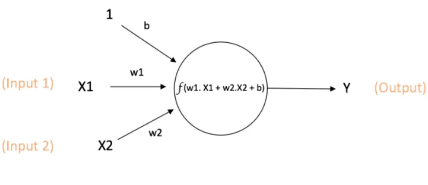
A neuron, also called a node or a unit is the simplest computation unit in a neural network. A neuron receives information or inputs from other nodes in the network or from external sources. Based on its relative importance to other inputs, every input has a weight w, assigned to it. The neuron then computes the output by applying a function to the weighted sum of its inputs. Figure 3 represents a neuron.

X1 and X2 with associated weights w1 and w2 are passed as inputs to the network. There is another input to the neuron called the Bias (b). The primary function of bias is to offer each node a constant value that is trainable, along with the inputs that the node gets normally.

1.2.3 The Activation Function (f)

The Activation Function (f), is non-linear and is used to add non-linearity to the neuron’s output.. Introducing linearity is very much needed as most of the data in the real world is non-linear and it is very important that the neurons learnthesenon-linear representations.

There are several activation functions.

• Sigmoid: A sigmoid function takes a real-valued number as input and produces an output

between zero and one.

• tanh: A tanh function takes a real-valued number as input and produces an output between

positive and negative one.

• ReLU: ReLU stands for Rectified Linear Unit. This function takes a real-valued number

as input and produces as output the maximum of zero or the input number. That is, it swaps negative numbers with zeros.

Figure 4 represents the graphs of various activation functions. We discuss the three most used activation functions.

Figure 4: Graphs representing various activation functions 1.2.4 Feedforward Neural Network

One of the very first neural networks devised is the Feedforward neural network. It contains multiple layers of nodes or neurons. Nodes from adjacent layers have edges or connections with certain weights associated between them. The information in a feed-forward neural network flows only in the forward direction. It starts at the input layer, flows through the hidden layer and to then reaches the output layer. Feed-forward neural network has no loops or cycles in it. Figure 5 represents a simple feedforward network.

1.2.5 Single-layer perceptron network

A Single-layer perceptron network is one of the simplest kinds of neural networks. A single-layer perceptron network consists only one layer of output nodes and the inputs with associated weights are directly fed to the output nodes. Each node computes the sum of the product of the weights and inputs and if the computed result is greater than a fixed threshold value (> 0), the neuron takes the activated value (generally 1), otherwise takes the deactivated value (generally -1).

Learning is achieved through a simple learning technique called the delta rule. The error between the expected output and the predicted output is calculated and the weights are adjusted based on this error. Figure 6 represents a single-layer perceptron network.

Figure 6: A single-layer perceptron network [25] 1.2.6 Multi-layer perceptron network

Multi-layer perceptron networks as the name suggests, consists of multiple layers of neurons. Neurons in all the layers are connected each other. Multi-layer networks use several different learning techniques and back propagation is the most used one among them.

In this learning technique, the predicted outputs are compared to the ground truth values and the error is calculated according to an error function that is predefined. This error is then fed into the system, using which, the weights of each input are adjusted with the aim to decrease the error by a small fraction. The same process is repeated for many iterations after which the model converges to a state where the error is small. With this, we could say that the model has learned a specific target function. Figure 7 represents a multi-layer perceptron network.

Figure 7: A multi-layer perceptron network [25]

In the next chapter, we study in detail about convolutional neural networks, their workings and how they are used in our model.

Chapter 2

Convolutional Neural Networks

Convolutional Neural Networks (CNNs) are a specific class of neural networks that perform exceptionally well in image classification and recognition and other computer vision tasks. Convolutional Networks have been very effective in identifying objects, human faces and traffic signals apart from rendering vision in self driving cars and robots.

In early 1980’s, Fukushima [1980] in his work on Neocognitron model [a], started experimenting with convolutional layers. He worked on character recognition problem with a convolutional layer along with a sub-sampling layer called the S-layer. He then classified images into various classes using this architecture. In the year 1998, LeCun et al. [29] used a few convolutional layers along with a few fully connected layers to identify digits that were handwritten. This model was named LeNet5 and was trained using complex algorithms such as backpropagation. Figure 8 represents a convolutional neural network model.

Figure 8: A convolutional neural network model [27]

All of the convolutional models will consist of the following four operations, which can be considered as the building blocks of CNNs:

1. Convolution

2. Non-Linearity (ReLU) 3. Pooling or Sub Sampling

4. Fully-connected Layer 2.1 Convolution

Any picture taken with a standard camera will represent the picture in three channels – blue, green and red. These channels can be imagined as a 2-D matrix with pixel values ranging from 0 to 255. In the case of a grey-scale image, we will have only one channel with pixel values ranging between 0 and 255, where values closer to 0 represent blacks and values closer to 255 represent whites. The main purpose of a convolution operation in convolutional neural networks is to collect image features from a given image. It learns the image features by preserving the spatial relationship between the image pixels.

Consider a 5x5 image with pixel values 0 and 1,

Consider a 3x3 matrix,

Now, the convolution of the 5x5 image with the 3x3 matrix can be calculated as:

is added as a value in the resultant matrix. The 3x3 matrix is called a ‘filter’ or a ‘kernal’. And the matrix that is the result of sliding the filter over the input image is called the ‘Feature Map’ or ‘Convolved Feature’. Different filter matrices generate different feature maps for the same input. That is different filters can extract different image features such as color information, boundaries and edges, pattern, etc.

The values of the filter are learned by the CNN model by its own during the training process, but the parameters such as filter size, number of filters, etc. should be specified before the training. As the filters are increased, more image features are extracted and more effective recognition of patterns is achieved.

Three parameters are used to tweak the size of the generated feature map: stride, zero-padding and depth.

• Stride: Stride corresponds to the count of pixels on which we move the filter over the input image.

• Zero-padding: Zero-padding lets us change and modify the size of the filter. To apply filter to the bordering elements of the image matrix, the border of the input matrix is padded with zeros.

• Depth: Depth is the count of filters used for the convolution operation. 2.2 Non-linearity: (ReLU)

ReLU stands for Rectified Linear Unit. ReLU is majorly used to add non-linearity in the network as majority of the real-world information that our convolutional network would learn would be non-linear. ReLU is applied per pixel and replaces every non-negative pixel value in the image by a zero. Figure 9 shows a graph that represents a ReLU function.

Figure 9: Graph representing ReLU function ReLU operation on an input image is represented by Figure 10.

Figure 10: ReLU operation on an input image [27]

ReLU nonlinearity performs best when compared to other non-linear functions such as sigmoid and tanh.

2.3 Pooling or Sub-sampling

Pooling or Sub-sampling retains the most important information from a feature map while reducing its dimensionality. It can be of various types: max pooling, average pooling, sum pooling, etc. Figure 11 represents the max pooling operation.

Figure 11: Max pooling operation [27]

In max pooling, a spatial region is defined and the maximum value from the feature map within that spatial region is considered. Rather than considering the maximum element, we could consider the average of all the elements in that region (average pooling) or take the sum of all the elements in that region (sum pooling). Max pooling performs best when compared to the rest. Figure 12 represents a max pooling operation on a given input image.

Figure 12: Max pooling operation on an input image [27] In addition to reducing the size of the input representation, pooling,

• controls overfitting by reducing the number of parameters and computations needed for processing.

• turns the model invariant to minor distortions and transformations in the image as we only consider either the max values or average values from the local neighborhood.

• outputs a scale-invariant representation of the image so that objects can be detected anywhere in the image.

2.4 Fully-connected layer

The results from the previous convolutional and spatial pooling layers represent the features of the image from a high level. These features are passed as input to the fully-connected layer which classifies the image into various predefined categories depending on the training data. The features that are extracted from the convolutional and pooling layers might work well for classification, but a combination of those features will give even better results. Adding a fully-connected layer is an effective way of learning these non-linear combinations.

By choosing to apply softmax function in the last layer of the fully-connected layer, it is ensured that the sum of probabilities from the fully connected layer is one. A sigmoid function takes a real-valued number as input and produces an output between zero and one, that sum to one. Figure 13 shows the layers in a convolutional neural network.

By summarizing all the operations and layers, the training phase in a convolutional neural network can be described in the following steps:

• Step 1: Use random values to initialize the weights, filters and parameters.

• Step 2: For a given training image as input, compute the output probabilities of each class with the forward propagation step (convolutional layer + ReLU + pooling layer + fully-connected layer).

• Step 4: Compute the gradients of the error with respect to all the weights in the model by using back propagation. Then adjust the weights, parameter and filter values to reduce the error. By this time, the model should be able to output the correct class of the given image. • Step 5: Reiterate steps 2-4 with the complete training set.

Figure 13: Layers in a convolutional neural network [27]

Given a training set that is considerably huge, the convolutional network will work well even with unseen images and will be able to put them correctly into their respective categories.

In the next chapter, we study about recurrent neural networks, precisely long short-term memory units, their internal workings and how they are used in our model.

Chapter 3

Recurrent Neural Networks

Recurrent neural networks (RNNs) are a special class of neural networks that were modelled to recognize patterns in sequences of data, such as handwriting, text, genomes, numerical data, or time-series data generated from stock markets, sensors, etc. Recurrent nets are arguably the most powerful class of networks modelled to identify structures in data sequences, such as, handwriting, times series data, text, speech, genomes or information generated from sensors, stock markets, IoT devices, etc.

Recurrent neural networks not only take the input at the current step as input but also what they have perceived in the previous step. The decision a recurrent neural network will reach at time t is affected by the decision it has reached at time t-1. We can say that there are two sources of input to a recurrent neural network, the present and the most recent past, based on which they take a decision on the new data. These networks differ from feed-forward neural networks by the feedback loop connected to their previous decisions; feeding the outputs back as input continuously. Recurrent networks make use of the information or knowledge present in the sequence itself to achieve tasks that feedforward networks cannot. Adding memory to the network makes all the difference.

Figure 14 represents a recurrent neural network being unfolded into a full network. Unfolding means representing the complete sequence of the network. For instance, if the complete sequence is a sentence of five words, the unfolded network would consist of 5 layers, one layer for each of the five words.

Figure 14: Unfolding of an RNN [28]

The computations occurring in an RNN are governed by the following formulae:

• 𝑥_" represents the input at time 𝑡. 𝑥_%could be a one-hot vector representing the 2nd word of the sentence.

• 𝑠" represents the memory and in turn the state of the network at time 𝑡. 𝑠" is derived by

considering the current input value and the previous hidden state: . The

function is a non-linear function such as ReLU or tanh.

• represents the output at step . The next word of a sentence could be predicted by considering

a vector of probabilities in our vocabulary .

3.1 Back Propagation Through Time (BPTT)

Backpropagation is the most common method used for training traditional neural networks. In feedforward networks, backpropagation assigns responsibility to the weights for a part of the error and moves backward from the error in the final layer through the weights, outputs and inputs of the hidden layers, by computing their partial derivatives - ∂E/∂w. Gradient descent then uses these derivatives to update the weights to minimize the error.

But simple backpropagation does not work in the case of training recurrent networks. The feedback loops in a recurrent network make it tricky. The problem with back propagating the error through a loop is that we cannot rely on the activations of the current time step of the network to determine how much a certain weight has affected the error. So, we must also back propagate through the time-state of the network and not just through the layers of the network to trace back the error. This variation or extension to the normal back propagation algorithm is called the “Back Propagation Through Time” or BPTT. The way BPTT works is that we unfold the recurrent network and keep an active memory of the activations in the previous neurons in the networks for a given number of time steps backward. If we want our network to have a memory of hundred time steps backward, then we unfold it into hundred copies of itself and apply simple backpropagation to this unfolded network. As we back propagate, the error and gradient for the weights is computed hundred times, one for each copy of the network. The average of these hundred gradients gives the true gradient of the network.

3.2 The Problem of Vanishing Gradient

To be able to back propagate the error through time, a correction term needs to be applied that enables us to propagate the error through the activation function at the output of each neuron. As we apply this correction term to each layer of the network, the correction terms begin to add up. Not just add up but they multiply up and this gives way for big problems since the correction terms are usually greater than one or less than one.

If the correction terms are greater than one, the gradients tend to explode, causing “The Problem of Exploding Gradient”. Diagonally, if the correction terms are less than one, the overall gradient decays to zero and eventually ‘vanishes’. Hence the name “The Problem of Vanishing Gradient”.

Therefore, we can only go so far back in time to train our recurrent network before the gradient is meaningless. And without a gradient or error signal, the network cannot learn anymore.

Once a certain threshold of depth is hit, back-propagation reaches its limit. A very creative solution was proposed by one Sepp Hochreiter in 1977 [10] to solve the vanishing gradient problem. This solution is a new RNN architecture called an LSTM network, is discussed in the following section. 3.3 Long Short-Term Memory (LSTM)

Long Short-Term Memory networks (LSTMs) are a unique subset of RNNs that creatively solve the vanishing gradient problem. In this network, a special cell called memory cell will store the input information for relatively longer duration of time. Unlike in the case of regular RNNs, where every node is just a regular node with an activation function, every node in an LSTM has the ability to store information. It also stores its own state. Figure 15 represents an LSTM memory cell. Traditional RNNs output a new hidden state by taking as input the old hidden state along with the current input. An LSTM does something similar but in addition to it, it takes its previous cell state as input and gives its new cell state.

Next, we study how an LSTM achieves to solve the vanishing gradient problem. There are three major steps:

1. The cell state is made to remember only important parts of the previous cell state and forget irrelevant parts.

2. Depending on the new input, the cell state is updated selectively.

Figure 15: An LSTM memory cell [29]

The steps mentioned are achieved through three gates: forget gate, input gate and output gate. Figure 16 represents the gates in an LSTM memory cell.

• Forget gate: A function of the current input and the previous hidden state are passed through the forget gate. For those sections of the state that are important to be stored, the forget gate outputs values close to 1 and for those parts that we wish to discard it outputs values closer to 0.

• Input gate: A function of the inputs is passed as input to the input gate, which is added to the cell state.

• Output gate: The values from the current cell state that are to be added to the hidden state output are decided by the output state.

The two main reasons why an LSTM overcomes the vanishing gradient problem are:

First: We know that the derivative of a sigmoid function is always less than 0.25 and when the 𝑓′(𝑥) ⋅ 𝑊 terms are multiplied together, the gradient vanishes away. But if we consider the case of an LSTM, its cell state is multiplied only with the output of the forget gate. So, function 𝑓 is considered as weights for the cell state. And besides the identity function itself, there is no other activation function. The identity function always has a derivative equal to one. And when 𝑓 equals one, information will be able to pass through this step unaltered.

Second: Observe that in the second step, the cell state is adjusted by adding some function of the inputs. And as we back propagate, and do the derivative of 𝐶" with respect to 𝐶"/%, the term that has been added, vanishes.

LSTMs have gained a lot of popularity in the field of natural language processing, as they have the capability of capturing long-term dependencies.

In the next chapter, we study in detail the solution approach and implementation details of our proposed model.

Chapter 4 Proposed Work

In this chapter, we formalize the task of visual question answering system and discuss the solution in detail.

4.1 Architecture

Our model uses a deep residual network (ResNet) to compute the image features and ByteNet to compute question embeddings. Depending on the question embeddings, a soft attention mechanism is applied, which generates multiple glimpses of most relevant image features. and a classifier is used to generate probabilities over an answer set. These glimpses along with the final state of ByteNet are passed as input to a classifier that generates probabilities over a set of answers. Figure 17 represents the architecture of our model.

Figure 17: Proposed architecture of our model

In our approach, the task of visual question answering is considered as a traditional classification problem. Given an input image 𝐼 and natural language question 𝑄,an answer 𝐴 is predictedfrom a set of answers Â, depending on the image content.

Our model is composed of three main components:

1. First component is the image model, which computes vectors for different regions of the image using ResNet, a CNN model.

2. The second component is the question model, which has convolutional neural network model or a long short-term memory unit to encode the semantics of the given question. 3. The third is the stacked attention model, which identifies relevant image regions according

to the semantics of the question. 4.1.1 Image Model

To compute a high-level representation 𝑓_@ of the given image 𝐼, we use ResNet, which is a residual network architecture based CNN pretrained on the ImageNet dataset.

𝒇𝑰= 𝑪𝑵𝑵𝑹𝒆𝒔𝑵𝒆𝒕(𝑰)

𝑓@ is a tensor (three-dimensional) which is taken from the final layer of ResNet, just before the last sub-sampling layer of 14 X 14 X 2048 dimensions. This is done to preserve the spatial information of the images. To further increase the learning dynamics, 𝑙I normalization is performed on the depth dimension of the image features.

4.1.2 Question Model

The given natural language question 𝑄 is then tokenized and converted into word embeddings 𝑊_J = { 𝑤_%, 𝑤_I, … … … . . 𝑤_N} where 𝐿 is the number of words in 𝑄. 𝑊_J is then passed as input to the ByteNet.

𝒇_𝑸 = 𝑪𝑵𝑵_{𝑩𝒚𝒕𝒆𝑵𝒆𝒕}(𝑾_𝑸) The final state of the ByteNet is used to represent the question.

4.1.3 Stacked Attention Network

Very few design choices have been found to improve the overall accuracy of neural network models consistently. One such design idea is the attention mechanism, which allows the neural networks to compute localized image features. Considering all the image and question features may add noise to more relevant areas of the image. This limitation is addressed through attention-based models, which focus on the most relevant areas of the image.

In our approach, the image embedding 𝑓_@ of fixed size of 14x14x2048 and the question embedding 𝑓_J of variable size are passed as inputs to the model. The word embedding vector is concatenated with different image features to form a single vector for each region. This single vector representation has the entire question semantics and the localized region of the image. A series of convolution and relu layers are applied on the concatenated vectors. The first section of convolution and relu layer will identify the relevant areas of the image based on the question. The second convolution layer will output a vector by emphasizing the selection regions which were identified in the previous section. We then apply a softmax function which takes in the output of the second convolution layer and generates a condensed vector representation of the concatenated vectors which are then passed on to the weighted average layer.

Using a weighted sum, this attention distribution is then fed the image feature vector to include various spatial feature regions. This produces a focused representation of the image that focuses on the most relevant spatial areas of the image when compared to other areas. This focused image feature vector is then fused with the question representation vector and passed through a softmax layer which outputs the answer. The same process is repeated using multiple stacked attention layers to address more complicated questions.

4.2 Feature Extraction

The models used for extracting image and question features are getting better and better as the time progresses. In our approach, comparatively simpler CNN architecture VGG16 is replaced with a sophisticated and advanced neural network architecture called ResNet, and LSTM is replaced with ByteNet to increase the performance and accuracy of VQA.

4.2.1 Image Feature - ResNet:

It is known that any function can be represented by a simple multi-layer perceptron network, given sufficient computing power. But this may lead to overfitting as the layer might become too huge. Therefore, networks with more deeper layers are preferred. However, as the number of layers increase and the network becomes deeper, the harder it becomes to train. This is mainly attributed to two problems. First: the vanishing gradient problem - as the depth increases, the gradient gathered at the last layer by comparing the prediction outputs with the actual outputs starts vanishing as we go deeper towards the early layers. Second: by increasing the parameter space and adding more layers, it is intuitive to think that our model learns better, which is not the case. Experiments have proven that more layers hike up the training error and degrade the performance of a model. This is called the degradation problem. Figure 18 shows how residual networks solve this problem by using residual blocks.

4.2.1.1 Residual Network

The residual block solves the degradation problem by connecting the feed forward networks in stages which are called ‘shortcut connections’. The advantage of using these ‘shortcut connections’ is that they solve the degradation problem and does not add up the complexity.

Figure 18: A residual block in ResNet [30] The shortcut connections in the residual block are of two types:

1. When the dimensions of the output and input are equal, identity (x) could be used.

The equation represents the residual equation when both output and input have equal dimensions.

2. When the inputs and outputs do not have equal dimensions,

a) Identity mapping is still achieved by the shortcut, by padding the dimension with zeroes.

b) The following formula is used by the projection shortcut to get the same dimension.

The equation represents the residual equation when both output and input do not have equal dimensions.

These identity mappings will provide better approximation when multiple non-linear layers are stacked together. The residual blocks will solve the degradation problem by simply deriving the weights of multiple non-linear layers using the identity mappings.

4.2.2 Question Features - ByteNet 4.2.2.1 LSTM (RNN) Vs Bytenet (CNN)

Recurrent neural networks, particularly LSTMs, have reshaped the field of natural language processing. In a language modeling task, the distribution of sequences of characters or words is estimated. RNNs although being the most used neural networks for this task, have a drawback. Inherently, the structure of recurrent networks is serial. Given a sequence as input, they manage sentences word-by-word. This serial structure of the RNNs is an obstacle that prevents parallelization. When the input is too huge, the content of distant locales in the sequence is lost. Also, to traverse from one token to another token in the sequence, complete serial path needs to be traversed by the backward and forward signals. And when the distance is large, the dependencies among the tokens is hard to learn. One solution to overcome this limitation is to use convolution networks instead of recurrent neural networks. Convolutions enable parallelization as they have no dependencies on the outputs at each layer as compared to recurrent networks.

4.2.2.2 Bytenet Architecture

The ByteNet is a convolutional neural network with one-dimension. The input sentence is encoded using convolutional layers.

• Encoder: The encoder is used to encode the input sequence. It is formed of convolutional layers of one-dimension that are not masked but use dilation. It processes the input string into a representation.

Conventionally, to decode the encoded sequence a decoder is used. Decoder will have the same convolutional layers with one-dimension that are masked and do not use dilation. Figure 20 represents the architecture of the ByteNet. The blue section represents the decoder which is placed over the encoder which is represented in red.

Figure 19: Architecture of the ByteNet [31] 4.2.2.3 Encoder-Decoder Stacking

The way in which the encoder and decoder are connected plays an important role in the architecture of ByteNet. To be able to preserve the temporal resolution of the sentence, the decoder is stacked over the encoder. This maximizes the bandwidth between the encoder and decoder. The different lengths of the inputs and outputs can be processed by a mechanism called dynamic unfolding, which allows the decoder to dynamically unfold on top of the encoder. This avoids the fixed-size compression of the input representation.

The ByteNet model has two principles which govern the behavior of the model. The stacking of encoder and decoder ensures that the runtime is linear with the size of the input sequence. This also avoids the necessity for heavy memorization. Dynamic unfolding guarantees performance irrespective of the length of the sentence. These advantages make ByteNet a simple and efficient solution for any natural language problem. Since the question-answering task involves multiple

stages of feature representation, ByteNet is the best choice for its efficient encoding state-of-the performance.

In the next chapter, we study the various datasets that are openly available for visual question answering, their strengths and limitations. We also study the various evaluation metrics used for evaluating the datasets.

Chapter 5

Datasets and Evaluation Metrics 5.1 Datasets for VQA

An ideal dataset for VQA should be large enough to capture the variations in questions, answers, images, objects and concepts in real world. It should have an evaluation metric that is

fair and achieving good results on it indicates that the algorithm can generate accurate answers to a wide variety of questions. In the following subsections, we review the available datasets and their strengths and limitations.

5.1.1 DAQUAR

The DAtaset for QUestion Answering on Real-world images (DAQUAR) [20], was one of the very first datasets to be released for VQA. It is also one of the smallest datasets. It consists of 6795 training and 5673 testing QA pairs based on images from the NYU-DepthV2 Dataset. The questions in this dataset majorly fall into three major categories. – objects, color of objects and number of objects. Most of the questions have single-word answers. Even though DAQUAR was the major dataset for VQA, the small size of it makes it difficult to train and evaluate complex models.

5.1.2 COCO-QA

In COCO-QA, an NLP algorithm is used to generate question-answer (QA) pairs for

images, from the COCO image captions. For example, for an image caption that says ‘The girl is crying’, the algorithm generates the question – ‘What is the girl doing?’ with the answer to it being ‘crying’. COCO-QA contains 78,736 training QA pairs and 38,948 testing QA pairs. COCO-QA contains 78,736 training and 38,948 testing QA pairs. The questions in this dataset fall into four major categories: object, color, number and location based with ratios being 70%, 17%, 7% and

6% respectively. All questions in the COCO-QA dataset have single word answers which makes it easier for evaluation. One limitation of the COCO-QA dataset is that the questions have many grammatical errors and are phrased awkwardly.

5.1.3 The VQA Dataset

VQA dataset is a combination of two datasets – COCO-VQA and SYNTH-VQA. COCO-VQA consists of real world images from COCO dataset, with three questions per image, and ten answers per question. In comparison to other VQA datasets, COCO-VQA has a relatively large number of questions - 614,163 total, with 248,349 for training, 121,512 for validation, and 244,302 for testing. SYNTH-VQA consists of 50,000 synthetic scenes that illustrate cartoon images in various simulated scenarios. It has 150,000 QA pairs with 3 questions per scene and 10 ground truth answers per question. A more balanced and diverse dataset is created by using synthetic images. The questions in this dataset fall into three major categories: open-ended questions, yes/no questions and number based questions. Due to the size and diversity of the dataset, the VQA Dataset has been widely used to evaluate algorithms.

5.2 Evaluation Metrics

VQA can be modeled as an open-ended task, where the questions are open ended or as a multiple-choice task where the algorithm has to choose the correct answer from the set of possible answer options. For multiple-choice VQA, simple accuracy can be used as an evaluation metric, where the answer is right when the algorithm makes the right choice. For open-ended VQA, the predicted answer should exactly match the ground truth answer string. However, simple accuracy is a very stringent metric. Hence various alternative evaluation metrics have been proposed to evaluate open-ended visual question answering.

Wu-Palmer Similarity (WUPS) proposed in [20], tries to measure how much a predicted answer differs from the ground truth based on the difference in their semantic meaning. Another alternative which was done for The VQA Dataset [12] and DAQUAR [15], is to have multiple ground truth answers for each question, collected independently. In DAQUAR, every question has five ground truth answers, annotated by humans. In VQA Dataset, every question has ten ground truth answers, annotated by humans. The metric used for evaluation is given by:

AccuracyVQA = min (n/3 , 1)

where n represents the number of annotators that marked the same answers as the algorithm. Figure 21 represents a table that compares the various evaluation metrics proposed for VQA.

Chapter 6

Experiments and Results 6.1 System Configuration

The system configuration that has been used for the experimental setup is detailed in Table 1. TABLE 1. System configuration

Specification Value

Operating System Ubuntu 14.04

Processor Intel(R) Xeon CPU E-2603 v5 @ _2.62GHz Graphic Processing Unit GeForce GTX 1080

Disk Space 2 TB

RAM (Memory) 64 GB

Programming Language Python 2.7

Tensorflow Version 1.6

Other librarries

6.2 Model Configuration and Training

The default model configuration that has been used for conducting all the experiments is mentioned in the following paragraph:

A 152 layer ResNet model which is pretrained on the ImageNet dataset is used to extract the image features. The final layer of ResNet (block 4), just before the last sub-sampling layer of 14 X 14 X 2048 dimensions is taken and 𝑙_I normalization is performed on the depth dimension. The question is tokenized and the question embeddings are represented by a D = 300 vector dimension. The

ByteNet with the state size set to 1024. The dropout value of the convolutional layers and fully-connected layers is set to 0.5. Adam optimizer with a batch size of 128 for 100K steps is used to optimize the model. The CNN parameters are kept constant during the training phase.

6.3 Model Parameters

Improving the performance of a model could be achieved by tweaking various hyper parameters in a neural network. Our model involves two convolutional neural networks. A combination of the hyper parameters from each of these models is tweaked and the performance of the model is evaluated. All model variations use the training set of VQA 1.0 for training and the validation set of VQA 1.0 for evaluation. The accuracy equation mentioned in the previous section is used to compute the accuracies. Table 2 shows the improvements in accuracies for the specified number of iterations for each hyper parameter tuned. The accuracies that are reported are taken before any overfitting has occurred and are represented in percentages.

TABLE 2. Accuracies reported by tuning various hyperparameters

Number of Steps 1K 3K 25K 50K 100K 200K

Our Model - Default

(ResNet+ByteNet) 37.35 46.33 52.68 60.31 60.91 60.96 No 𝒍_𝟐 normalization 42.35 44.75 50.72 51.95 54.39 54.57 No dropout on FC/CNN layers 32.78 37.87 57.50 57.12 57.35 56.86 No dropout on ByteNet 46.65 51.53 59.45 59.93 59.97 59.85 No attention 37.68 47.26 56.10 57.22 57.45 57.68

From the results, we observed that applying l2 normalization on the ResNet features resulted in a much lower training time and improved accuracy. Using dropout on the convolutional and fully-connected layers contributed a lot in avoiding over fitting. We also observed that there was a

6.4 Model Variations

During evaluation, we conducted experiments on our original ResNet and ByteNet model, represented by Our Model (ResNet+Bytenet) and also by replacing the ResNet and ByteNet in our model with a few available alternatives to compare the performances. We experimented with the following variations of our model:

• Our Model (ResNet + ByteNet) • Our Model (VGG16 + ByteNet) • Our Model (ResNet + LSTM) • Our Model (VGG16+ LSTM)

For evaluation, we have used the validation set of VQA 1.0 dataset. Table 3 shows a comparison Our Model (ResNet+ByteNet) with the different model variations that we experimented with. All accuracies are represented in percentages.

TABLE 3. Comparison of our default model with variations of our model on VQA 1.0

Model Yes/No Number Other All

Our Model (VGG16+LSTM) 79.3 36.6 46.1 58.7 Our Model (VGG16+ByteNet) 79.8 37.23 48.98 60.21 Our Model (ResNet+LSTM) 80.12 38.1 49.28 63.12

Our Model – Default

(ResNet+ByteNet) 82.2 39.1 55.2 64.5

From the results reported in Table 3 it is evident that there is a significant improvement in the accuracies when VGG16 and LSTM are replaced by a ResNet and a ByteNet.

6.5 Datasets

Our model is evaluated on three of the widely-used image question answering datasets discussed in the previous sections. Table 4 represents the number of questions and images available in each of the datasets used.

TABLE 4: Question and image statistics in the datasets used

Dataset Questions - Train Questions - Test Images - Train Images - Test

DAQUAR-ALL 6, 795 5, 673 795 654

COCO-QA 78736 38948 8, 000 4, 000

VQA 248, 349 121, 512 123,287 81,434

6.6 Comparison to state of the art 6.6.1 DAQUAR-ALL

Table 5 shows a comparison of our model with the state of the art on the DAQUAR-ALL dataset. All accuracies are represented in percentages.

TABLE 5: Comparison of our model with the state of the art on DAQUAR-ALL

Model Accuracy Multi-World 7.9 Ask-Your-Neurons 21.7 IMG-CNN 23.4 Our Model (ResNet+ByteNet) 29.3

6.6.2 COCO-QA

Table 6 shows a comparison of our model with the state of the art on the COCO-QA dataset. All accuracies are represented in percentages.

TABLE 6: Comparison of our model with the state of the art on COCO-QA

Model Accuracy GUESS 6.7 BOW 37.5 LSTM 36.8 IMG 43.0 IMG+BOW 55.9 VIS+LSTM 53.3 IMG-CNN 55.0 CNN 32.7 Our Model (ResNet+ByteNet) 61.6

Table 7 shows the results of accuracies for various classes of questions in the COCO-QA dataset. All accuracies are represented in percentages.

TABLE 7: COCO-QA accuracies for various question types

Model Objects Number Color Location

GUESS 2.1 35.8 13.9 8.9 BOW 37.3 43.6 34.8 40.8 LSTM 35.9 45.3 36.3 38.4 IMG 40.4 29.3 42.7 44.2 IMG+BOW 58.7 44.1 52.0 49.4 VIS+LSTM 56.5 46.1 45.9 45.5 Our Model (ResNet+ByteNet) 64.5 48.6 57.9 54.0

6.6.3 The VQA Dataset VQA 1.0:

Table 8 shows a comparison of our model with the state of the art on the VQA 1.0 Dataset. The reported accuracies are for the various question types in the VQA 1.0 Dataset. All accuracies are represented in percentages.

TABLE 8: VQA 1.0 accuracies for various question types

Model Yes/No Number Other All

VQA Team 80.5 36.8 43.1 57.8 SAN (VGG) 79.3 36.6 46.1 58.7 ACK (VGG) 81.0 38.4 45.2 59.2 DAN (VGG) 82.1 38.2 50.2 62.0 MRN (ResNet) 82.3 38.8 49.3 61.7 MCB (ResNet) 82.2 37.7 54.8 64.2 DAN (ResNet) 83.0 39.1 53.9 64.3 Our Model (ResNet+ByteNet) 82.2 39.1 55.2 64.5 VQA 2.0:

Table 9 shows a comparison of our model with the state of the art on the VQA 1.0 Dataset. The reported accuracies are for the various question types in the VQA 1.0 Dataset. All accuracies are represented in percentages.

TABLE 9: VQA 2.0 accuracies for various question types

Model Yes/No Number Other All

HieCo Att 71.80 36.53 46.25 54.57

MCB 77.37 36.66 51.23 59.14

Our Model

(ResNet+ByteNet) 77.45 38.46 51.76 59.67

6.7 Error Analysis

To perform error analysis, we selected 100 random images from the VQA validation dataset on which our model failed to predict correct answers. We observed that the errors can be broadly categorized into four types:

i. Incorrect attention areas were highlighted (37%) Question: What is the color of the background?

ii. Correct attention region but incorrect answer prediction (23%) Question: How many umbrellas are there?

Predicted Answer: Two Ground Truth: Three

iii. Different labels but almost correct answer predictions (21%) Question: What is the object?

Predicted Answer: Pot Ground Truth: Vase

iv. Incorrect labels with correct answer predictions (19%) Question: What color is the train?

Chapter 7

Conclusion and Future Work

In this work, we proposed a new baseline for the task of visual question answering. Our model uses a deep residual network (ResNet) to compute the image features and a dilated convolutional network (ByteNet) to compute question embeddings. A soft attention mechanism is used to focus on most relevant image features and a classifier is used to generate probabilities over an answer set.

Prior to using deep residual networks, we tried using VGG16 for extracting image features. From the results in the previous section, we observed that using ResNet for image feature extraction resulted in a significant increase in the accuracy when compared to VGG16. We also implemented a variation of our model by replacing ByteNet with a long short-term memory unit (LSTM) and compared the accuracies. We evaluated our proposed model on the VQA 1.0 dataset by tweaking various hyper parameters of the CNN and RNN models and observed how various hyper parameters are affecting the accuracy of the model. We then evaluated our model on three benchmark datasets for image question answering and compared the results with the state of the art. Our model, despite having a relatively simple architecture, achieves 64.6% accuracy on VQA 1.0 dataset and 59.7% accuracy on VQA 2.0 dataset.

As a future extension of this work, we might want to extend our model to answer open-ended questions on multiple images rather than a single image. The motive behind a multi-image question answering system is to gather the context from multiple images and be able to answer open-ended questions on a sequence of images. This could be used as a base for video question answering system which can be used in a video surveillance system.

REFERENCES

[1] J. Redmon, S. Divvala, R. Girshick, and A. Farhadi, “You only look once: Unied, real-time object detection," in The IEEE Conference on Computer Vision and Pattern Recognition (CVPR), 2016.

[2] S. Ren, K. He, R. Girshick, and J. Sun, “Faster r-cnn: Towards real-time object detection with region proposal networks," in Advances in Neural Information Processing Systems (NIPS), 2015. [3] K. Simonyan and A. Zisserman, “Very deep convolutional networks for large-scale image recognition," in International Conference on Learning Representations (ICLR), 2015.

[4] K. He, X. Zhang, S. Ren, and J. Sun, “Deep residual learning for image recognition," in The IEEE Conference on Computer Vision and Pattern Recognition (CVPR), 2016.

[5] J. Donahue, L. A. Hendricks, S. Guadarrama, M. Rohrbach, S. Venugopalan, K. Saenko, and T. Darrell, “Long-term recurrent convolutional networks for visual recognition and description," in The IEEE Conference on Computer Vision and Pattern Recognition (CVPR), 2015.

[6] A. Karpathy and L. Fei-Fei, “Deep visual-semantic alignments for generating image descriptions," in The IEEE Conference on Computer Vision and Pattern Recognition (CVPR), 2015.

[7] J. Mao, W. Xu, Y. Yang, J.Wang, Z. Huang, and A. Yuille, “Deep captioning with multimodal recurrent neural networks (m-rnn)," in International Conference on Learning Representations (ICLR), 2015.

[8] C. Szegedy, W. Liu, Y. Jia, P. Sermanet, S. Reed, D. Anguelov, D. Erhan, V. Vanhoucke, and A. Rabinovich, “Going deeper with convolutions," in The IEEE Conference on Computer Vision and Pattern Recognition (CVPR), 2015.

[9] K. Cho, B. Van Merri enboer, C. Gulcehre, D. Bahdanau, F. Bougares, H. Schwenk, and Y. Bengio, “Learning phrase representations using rnn encoder-decoder for statistical machine translation," in Conference on Empirical Methods on Natural Language Processing (EMNLP), 2014.

[10] S. Hochreiter and J. Schmidhuber, “Long short-term memory," Neural computation, vol. 9, no. 8, pp. 1735{1780, 1997}.

[11] R. Kiros, Y. Zhu, R. Salakhutdinov, R. S. Zemel, A. Torralba, R. Urtasun, and S. Fidler, A CNN APPROACH FOR VQA “Skip-thought vectors," in Advances in Neural Information Processing Systems (NIPS), 2015.

[12] S. Antol, A. Agrawal, J. Lu, M. Mitchell, D. Batra, C. L. Zitnick, and D. Parikh, “VQA: Visual question answering," in The IEEE International Conference on Computer Vision (ICCV), 2015.

[13] H. Gao, J. Mao, J. Zhou, Z. Huang, L. Wang, and W. Xu, “Are you talking to a machine? Dataset and methods for multilingual image question answering," in Advances in Neural Information Processing Systems (NIPS), 2015.

[14] K. Kafle and C. Kanan, “Answer-type prediction for visual question answering," in The IEEE Conference on Computer Vision and Pattern Recognition (CVPR), 2016.

[15] B. Zhou, Y. Tian, S. Sukhbaatar, A. Szlam, and R. Fergus, “Simple baseline for visual question answering," arXiv preprint arXiv:1512.02167, 2015.

[16] A. Fukui, D. H. Park, D. Yang, A. Rohrbach, T. Darrell, and M. Rohrbach, “Multimodal compact bilinear pooling for visual question answering and visual grounding," in Conference on Empirical Methods on Natural Language Processing (EMNLP), 2016.