Copyright by Bulent Guler
The Dissertation Committee for Bulent Guler
certifies that this is the approved version of the following dissertation:
Essays on Housing and Labor Markets
Committee:
P. Dean Corbae, Supervisor
Fatih Guvenen, Supervisor
Russell W. Cooper
Burhanettin Kuruscu
Essays on Housing and Labor Markets
by
Bulent Guler, B.S., M.A.
DISSERTATION
Presented to the Faculty of the Graduate School of The University of Texas at Austin
in Partial Fulfillment of the Requirements
for the Degree of
DOCTOR OF PHILOSOPHY
THE UNIVERSITY OF TEXAS AT AUSTIN May 2009
Dedicated to my wife Asli, my son Tarik and
Acknowledgments
I would like to thank my thesis supervisors Fatih Guvenen and P. Dean Cor-bae for their generous time and encouragement. I specifically owe a lot to Fatih Guvenen for his continuing support starting from the first day of my Ph.D. studies. With his leadership, research skills, hard work and scholarship, he has become a great role model for me. I am also very grateful for having an exceptional doc-toral committee. I want to thank to my committee members Gianluca Violante, Burhanettin Kuruscu and Russell Cooper for their support and fruitful conversa-tions.
My special thanks go to my wife Asli for her enormous support, understand-ing and patience, and of course to my son Tarik for beunderstand-ing the ultimate joy of my of life. I would also like to thank to my parents for their continuous support through my entire life.
Last but not least, I would like to thank Yavuz Arslan, Pablo Derasmo, Borghan Narajabad and Juan Sanchez for their valuable comments about my thesis.
Essays on Housing and Labor Markets
Publication No.
Bulent Guler, Ph.D.
The University of Texas at Austin, 2009 Supervisors: P. Dean Corbae
Fatih Guvenen
In the first chapter, I study the effects of innovations in information technol-ogy on the housing market. Specifically, I focus on the improved ability of lenders to assess the credit risk of home buyers, which has become possible with the emergence of automated underwriting systems in the United States in the mid-1990s. I develop a standard life-cycle model with incomplete markets and idiosyncratic income uncer-tainty. I explicitly model the housing tenure choice of the households: rent/purchase decision for renters and stay/sell/default decision for homeowners. Risk-free lenders offer mortgage contracts to prospective home buyers and the terms of these con-tracts depend on the observable characteristics of households. Households are born as either good credit risk types—having a high time discount factor—or bad types— having a low time discount factor. The type of the household is the only source of asymmetric information between households and lenders. I find that as lenders have better information about the type of households, the average downpayment fraction decreases together with an increase in the average mortgage premium, the foreclosure rate, and the dispersions of mortgage interest rates and downpayment
fractions, which are consistent with the trends in the housing market in the last 15 years. From a welfare perspective, I find that better information, on average, makes households better off.
In the second chapter, I focus on the labor market behavior of couples. Search theory routinely assumes that decisions about the acceptance/rejection of job offers (and, hence, about labor market movements between jobs or across em-ployment states) are made by individuals acting in isolation. In reality, the vast majority of workers are somewhat tied to their partners—in couples and families— and decisions are made jointly. This chapter studies, from a theoretical viewpoint, the joint job-search and location problem of a household formed by a couple (e.g., husband and wife) who perfectly pool income. The objective of the exercise, very much in the spirit of standard search theory, is to characterize the reservation wage behavior of the couple and compare it to the single-agent search model in order to understand the ramifications of partnerships for individual labor market outcomes and wage dynamics. We focus on two main cases. First, when couples are risk averse and pool income, joint-search yields new opportunities—similar to on-the-job search—relative to the single-agent search. Second, when couples face offers from multiple locations and a cost of living apart, joint-search features new frictions and can lead to significantly worse outcomes than single-agent search.
Finally, in the third chapter, I focus on the relation between house prices and interest rates. Although interest rates and housing prices seem mostly to have a negative relation in the data, the relation does not seem to be stable. For example, the recent run up in the global housing prices is generally explained by globally low
interest rates. On the other hand, there have been periods where housing prices and interest rates moved together. Motivated by these observations, I formulate a two period OLG model to find out the form of the relationship between interest rates and housing prices. It appears that the distribution of homeownership is also important for housing price dynamics. I show that housing prices in the equilibrium do not always have a negative relation with interest rates.
Table of Contents
Acknowledgments v
Abstract vi
List of Tables xii
List of Figures xiii
Chapter 1. Innovations in Information Technology and the Mortgage
Market 1
1.1 Introduction . . . 1
1.2 Innovations in Information Technology . . . 8
1.3 Model . . . 11 1.3.1 Environment . . . 11 1.3.1.1 Households . . . 13 1.3.1.2 Lenders . . . 16 1.3.1.3 Timing . . . 16 1.3.1.4 Information Structure . . . 18 1.3.2 Decision Problems . . . 18 1.3.2.1 Household’s Problem . . . 19 1.3.2.2 Lender’s Problem . . . 25 1.3.3 Equilibrium . . . 29 1.4 Findings . . . 32 1.4.1 Calibration . . . 32 1.4.2 Results . . . 36
1.4.3 Counterfactual: The Effect of the Information Structure . . . 41
1.4.4 Alternative Equilibrium Concept . . . 54
Chapter 2. Joint-Search Theory: New Opportunities and New
Fric-tions 61
2.1 Introduction . . . 61
2.2 The Single-Agent Search Problem . . . 65
2.3 The Joint-Search Problem . . . 67
2.3.1 Characterizing the couple’s decisions . . . 70
2.3.2 Risk-neutrality . . . 73
2.3.3 Risk-aversion . . . 75
2.3.3.1 CARA utility . . . 76
2.3.3.2 DARA utility . . . 80
2.3.3.3 IARA utility . . . 84
2.3.4 An Isomorphic Model: Single-Search with Multiple Job Hold-ings . . . 86
2.4 Extensions . . . 87
2.4.1 Nonparticipation . . . 88
2.4.2 On-the-job search . . . 91
2.4.3 Exogenous separations . . . 94
2.4.4 Borrowing in Financial Markets . . . 96
2.4.5 Some illustrative simulations . . . 100
2.5 Joint-search with Multiple Locations . . . 105
2.5.1 Two locations . . . 107
2.5.2 Some illustrative simulations with multiple locations . . . 114
2.6 Conclusions . . . 118
Chapter 3. House Prices and Interest Rates 120 3.1 Introduction . . . 120
3.2 The Model . . . 124
3.3 Solution of the Model . . . 130
3.3.1 Case 1: π = 0: Agents don’t move . . . 130
3.3.2 Case 2: π = 1: All agents move . . . 132
3.3.3 Case 3π∈(0,1): Some agents move . . . 134
3.4 Calibration . . . 137
3.5 Results . . . 139
Appendices 145
Appendix A. Chapter 1 Appendix 146
A.1 Existence of Equilibrium - A Simplified Model . . . 146
Appendix B. Chapter 2 Appendix 154
B.1 Proofs . . . 154 B.2 Additional value functions . . . 171
Bibliography 174
List of Tables
1.1 Summary Statistics . . . 2 1.2 Calibration . . . 33 1.3 Benchmark Results - Symmetric Information vs Asymmetric
Infor-mation . . . 38 1.4 Counterfactual-The Effect of the Information Structure . . . 42 2.1 A Comparison of Single- versus Joint-Search with CRRA Preferences 102 2.2 Single- versus Joint-Search: CRRA Preferences and On-the-Job Search105 2.3 Single- versus Joint-Search: 9 Locations and Risk Neutral Preferences 115 3.1 Calibrated Parameters . . . 139
List of Figures
1.1 Mortgage Interest Rate as a Function of Loan Amount . . . 43
1.2 Mortgage Interest Rate in Both Economies . . . 46
1.3 Homeownership Rate over the Life Cycle in SI vs AI . . . 47
1.4 Foreclosure Rate over the Life Cycle in SI vs AI . . . 47
1.5 Mean Income of Homeowner over the Life Cycle in SI vs AI . . . 50
1.6 Mean Income of Renter over the Life Cycle in SI vs AI . . . 50
1.7 Debt-to-Income Ratio over the Life Cycle in SI vs AI . . . 52
1.8 Debt-Service Ratio over the Life Cycle in SI vs AI . . . 52
1.9 Consumption of Homeowner over the Life Cycle in SI vs AI . . . 55
1.10 Consumption of Renter over the Life Cycle in SI vs AI . . . 55
2.1 Reservation Wage Functions of a Risk-Neutral Couple: Search be-havior is identical to the single-search economy. . . 74
2.2 Reservation Wage Functions with CARA Preferences. . . 77
2.3 Simulated Wage Paths for a Couple (Joint-Search) and for Same In-dividuals When they are Single. . . 81
2.4 Reservation Wage Functions with DARA Preferences (CRRA is a Special Case). . . 83
2.5 Reservation Wage Functions with IARA Preferences (Quadratic Util-ity is a Special Case). . . 85
2.6 Reservation Wage Functions for Outside Offers with Risk-Neutral Preferences and Two Locations . . . 110
2.7 Reservation Wage Functions forInside Offers with Risk-Neutral Pref-erences and Two Locations . . . 110
2.8 Tied-Stayers and Tied-Movers in the Joint-Search Model . . . 113
3.1 Median House Prices . . . 121
3.2 30 Year Real Fixed-Rate Mortgage Rates. . . 122
3.3 Change in Housing Prices vs Change in Mortgage Rates . . . 123
3.5 The Constant Term in the Housing Demand Function . . . 140
3.6 The Coefficient ofHt−1,y in the House Demand Function . . . 141
3.7 The Constant in the Housing Price Function . . . 142
3.8 The Coefficient ofHt−1,y in the Housing Price Function . . . 143
3.9 Equilibrium House Price: The Effects of Supply and Demand . . . . 144
Chapter 1
Innovations in Information Technology and the
Mortgage Market
1.1 Introduction
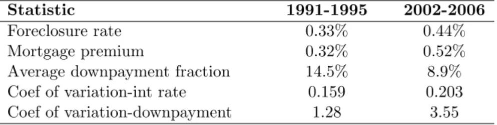
The US housing market has witnessed important changes since the mid-1990s. Arguably, the most prominent technological change during this time was the emergence of automated underwriting systems (hereafter AUS), which allowed a better assessment of the credit risks of home buyers. In particular, advances in in-formation technology (e.g., the rapid decline in the cost of storing and transmitting credit information) have enabled access to more comprehensive data on households, which in turn increased the predictive power of credit scores, thereby allowing lenders to assess the credit risk of home buyers more precisely. Accompanying these im-provements in information technology, the housing market has experienced changes along some key dimensions. As reported in Table 1.1, a comparison of the 1991-1995 period and 2002-2006 period reveals that (i) the foreclosure rate has increased, (ii) average mortgage premium has gone up, (iii) average downpayment fraction has decreased, and (iv) the dispersions of mortgage interest rates and downpayment fractions have risen up.
Table 1.1: Summary Statistics*
Statistic 1991-1995 2002-2006
Foreclosure rate 0.33% 0.44%
Mortgage premium 0.32% 0.52%
Average downpayment fraction 14.5% 8.9% Coef of variation-int rate 0.159 0.203 Coef of variation-downpayment 1.28 3.55
* Downpayment and mortgage interest rate data are from American Housing Survey
and calculated for 30-year fixed rate mortgages. Mortgage premium, measured as the difference between 30-year fixed rate mortgage and AAA corporate bond yield, is from Federal Reserve Board. Foreclosure data is from Mortgage Bankers Association.
In this paper, I explore the effect of innovations in information technology— specifically, the increased ability of lenders to assess the credit risk of home buyers— on the housing market. I develop a standard life-cycle model with incomplete mar-kets and idiosyncratic labor income uncertainty. I also model the housing tenure choice. There are two types of households: those with a high time discount factor (ie., the “good” type) and those with a low time discount factor (ie., the “bad” type). Households are born as renters with ex-ante heterogeneity in income and wealth. Every period, renters decide whether or not to purchase a house. There is a continuum of risk-neutral lenders who offer mortgage contracts to prospective home buyers. A mortgage contract consists of a mortgage interest rate, loan amount, mortgage repayment schedule and maturity. Mortgages are fully amortizing, that is, homeowners have to pay the mortgage back in full until the end of the mortgage contract, as specified by the maturity. However, homeowners also have the option to sell their houses or default on the mortgage and return to the rental market. Selling a house is different from defaulting, because a seller has to pay back the outstanding mortgage balance to the lender whereas a defaulter has no obligation. Therefore,
de-fault occurs in equilibrium as long as the selling price is lower than the outstanding mortgage debt. Upon default, the household becomes a renter again and is excluded from the mortgage market for a certain number of years as punishment.
There is free entry into the credit market, so in equilibrium lenders make zero profit on each contract. Since mortgages are long-term contracts, it is essential for the lenders to infer the default probability of each household at every date and state, which depends on the income risk as well as on the type of each household. Clearly, given an income realization, a household with a low time discount factor (bad type) has a higher probability of default, since she values the benefit of homeownership less compared to the good types. I explore two information structures. In one economy, lenders cannot observe the types although they can observe all the other characteristics of the household. This creates asymmetric information between the lenders and households, and I call this the asymmetric information economy (AI). In the other economy, lenders can observe all the characteristics of the household and therefore information is symmetric (hence, called symmetric information economy, SI).1
I interpret the AI economy as representing the US economy before the emer-gence of automated underwriting systems (before mid-1990s), whereas the SI econ-omy represents the more recent period with AUS (mid-2000s). Because these two
1
Chatterjee, Corbae and Rios-Rull (2007, 2008) build a model of reputation in credit markets and show how credit scores are informative about the type of the households in equilibrium. Good types are patient and value reputation more compared to the bad types. As a result, the credit score, which tracks the history of the ability and willingness of the household to make debt pay-ments, becomes very informative in differentiating the households. However, due to the curse of dimensionality of such a model, I do not explicitly model the credit scores. Instead, I assume that the emergence of credit scores has enabled lenders to fully observe the type of the households.
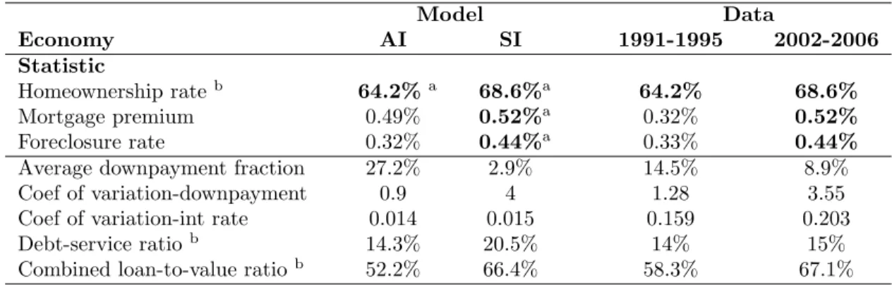
time periods also differ in average interest rates and housing prices, each economy is calibrated to match these two empirical targets in their respective time period. The results indicate that the transition from the AI economy to the SI economy decreases the downpayment fraction and increases the mortgage premium, foreclo-sure rate, and homeownership rate, which are consistent with the current changes in the mortgage market. Moreover, consistent with the data, the transition brings an increase in the dispersion of the mortgage interest rates and downpayment fractions. However, the levels of the dispersion of mortgage interest rates that the model gen-erates are much lower than their data counterparts. This is mainly due to omission of several important risk factors (i.e., risk-free interest rate risk, house price risk) in the model.
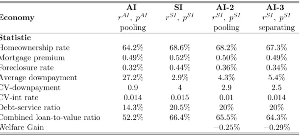
Because the AI and SI economies also differ in the average interest rate and housing price, I conduct the following (counterfactual) experiment to isolate the role of information technology. Basically, I simulate the AI economy with the same set of parameters in the SI economy. The results show that information structure is the main driving force behind the increase in the dispersion of mortgage interest rates and downpayment fractions as well as having an important role in the increase of the mortgage premium, the foreclosure rate, and the decrease in the downpayment fraction. Risk-free interest rate and house price are more important in explaining the increase in the homeownership rate and the decrease in the downpayment fraction. A higher foreclosure rate does not mean that lenders and households are worse off in the SI economy. When I measure the welfare gain of being born into the SI economy as opposed to the AI economy, the gain, in consumption equivalent
terms, is between 0.25% and 0.29% depending on whether I use pooling contracts or separating contracts as equilibrium contracts in the AI economy. Furthermore, the zero-profit restriction on the contracts ensures that, ex-ante, lenders are indifferent between both economies. I, finally, check the robustness of the results to the selection of equilibrium in the AI economy. The counterfactual shows the equilibrium with pooling contracts. To explore the effect of an alternative equilibrium, I solve the AI economy with separating contracts. The new equilibrium with separating contracts shows very similar effects as the equilibrium with pooling contracts.
In the AI economy, lenders cannot observe the types and they face an ad-verse selection problem. This puts additional constraints on the contracts offered in the AI economy. The transition from the AI economy to the SI economy, both in the extensive margin and intensive margin, makes the credit terms more relaxed. In the extensive margin, those low income households who are rationed out in the AI econ-omy become eligible for mortgages. Since these households are income constrained, they demand for lower downpayment fraction which requires higher mortgage pre-mium. In the intensive margin, since bad types are, now, perfectly observed they get contracts that have lower downpayment fraction at the cost of higher mortgage premium2. Moreover, since good types face lower mortgage premium, they also demand for lower downpayment fraction loans. As a result downpayment fraction decreases whereas mortgage premium and homeownership rate increase. Since the
2
Note that households face a trade-off between the downpayment fraction - short-term debt - and mortgage payment - long-term debt - during the house purchase. Bad types - impatient households - favor a decrease in the downpayment fraction more than an decrease in the mortgage payment compared to the good types - patient households.
new home purchasers are low income households and average downpayment fraction decreases together with an increase in the mortgage premium, the default risk in the market increases. Thus, the foreclosure rate increases.
There is a growing empirical literature suggesting that innovations in the mortgage market are the main reasons for the recent changes in the housing market. Testing the forecasting relationship between housing spending and future income, Gerardi, Rosen and Willen (2006) find that recent developments in the mortgage market have ensured that households have been more able to buy houses whose values are in line with their long-term income prospects. Mian and Sufi (2008) document that high unfulfilled demand zip codes experienced relative declines in mortgage application denial rates and mortgage interest rates and relative increases in mortgage credit and house prices despite the negative relative income and em-ployment growth in these zip codes. They also find that the growth of securitization was significantly higher in high unfulfilled demand zip codes, suggesting a possible role of supply side changes in the mortgage market. Finally, using the American Housing Survey data, Doms and Krainer (2007) find that housing expenditures of the households facing the greatest financial constraints have increased substantially using, particularly, the newly designed mortgages.
Although, on the empirical side, financial innovations in the mortgage in-dustry and its impact on the market and households seem to be well documented, the literature thus far has paid little attention to modeling this link. In a stylized model, Ortalo-Magne and Rady (2006) show the effect of credit constraints, espe-cially the effect of downpayment requirement, on the extensive and intensive margin
of homeownership. Chambers, Garriga and Schlagenhauf (2008), in a quantitative framework, analyze the effect of financial innovations on the homeownership rate. They find that the key to understanding the increase in the homeownership rate, especially for young households, is the expansion of the set of mortgage contracts. Nevertheless, their way of modeling the terms of mortgage credit is in a reduced form and cannot explain the reason for the expansion of the mortgage credit. Moreover, they do not model the default option.
The equilibrium model of mortgage credit and default used in this paper is related to the equilibrium models of unsecured borrowing and bankruptcy3. Closely related to my paper are three papers influenced by Narajabad (2007): Sanchez (2008), Athreya, Tam and Young (2008), and Livhits, MacGee and Tertilt (2008) who explore the effects of innovations in the unsecured credit market. These papers show that a transition from a partial information economy to a full information economy results in an increase in consumer bankruptcies and debt which is consistent with the trend in the data. These papers analyze the unsecured credit market and borrowing is only for one period. Different from these models, I analyze the mortgage market characterized by secured borrowing and long-term maturity contracts which requires us to model the lender’s problem recursively.
This paper is organized as follows: Section 1.2 documents some recent in-novations in the mortgage market, especially focusing on the emergence of credit scoring technology and its impacts on the market. Section 1.3 describes the
envi-3
Chatterjee, Corbae, Nakajima (2007) and Livhits, MacGee and Tertilt (2007) are some promi-nent examples of such models.
ronment and sets up the model. Section 1.4 presents the main results of the model together with a counterfactual experiment separating the impact of the change in information structure. It also presents the results for an alternative equilibrium defi-nition. Finally, Section 1.5 concludes with directions for future work. The Appendix presents a simpler model to analyze the potential existence problem.
1.2 Innovations in Information Technology
There are three basic components of single-family mortgage underwriting: the value of the collateral, the ability of the borrower to make monthly mortgage payments and the willingness of the borrower to pay back outstanding mortgage debt. They are summarized as the traditional “three C’s”: Collateral, Capacity and Credit. The loan-to-value ratio is the measure of the collateral, which is basically measured by the downpayment fraction and the real value of the house. Capacity is useful to understand the ability of the borrower to make the monthly mortgage payments and is measured through several economic variables regarding the home buyer such as debt-to-income ratio, debt-service ratio,employment status, and sav-ings. Lastly, credit shows both the ability and willingness of the borrower to pay back the debt and is assessed through a credit report summarizing the historical performance of the home buyer in the credit market.
Until the mid 1990’s, credit was the missing piece of the three C’s. Insuf-ficient available credit data for individuals was the main reason for the absence of credit reports in mortgage underwriting. Unlike unsecured credit, mortgages are long-term contracts and larger amount of loans are at risk or fraudulent. Knowing
the ability of the home buyer to make the periodic mortgage payments is the most important information for the lenders. The home buyer’s loyalty to the payments strongly depends on his credit history, which captures the historical performance of the individual in the credit market. Borrowers with poor credit records go into mortgage default at much higher rates than borrowers with good credit records. Since insufficient credit report data may be misleading, lenders hesitated to use the credit reports for a long time. Straka (2000) shows the relationship between credit scores and default rates using a 1995 assessment of a large sample of Freddie Mac loans which were originated between 1990 and 1991. The result shows that in a weak regional housing market, a mortgage holder with a credit score, measured as a FICO score, smaller than 620 is 17 times more likely to default than a mortgage holder with a credit score higher than 760. He also shows that even in a strong regional housing market, credit scores have a great predictability of mortgage default4.
As the IT revolution has made computers part of our daily life, enabled data storage to become more efficient and less expensive and allowed computer net-working through local area networks and the internet, there has been an explosion in the growth of credit report in the late 1980s and early 1990s5. As a result we see a shift in the mortgage landscape. Long-time dominant manual and decen-tralized underwriting and origination systems requiring labor and paper intensive loan processing and risk assessment and lasting for weeks and even months have
4
See also Pennington-Cross (2003), Cutts and Green (2004) and Barakova, Bostic, Calem, and Wachter (2003) for further evidence of predictive power of credit scores in mortgage repayment and default.
5See Hunt (2005) on the evolution of consumer credit reports and Lacour-Little (2000) and
been rapidly replaced by automated and centralized underwriting systems based on credit scores, statistical model loan processing and risk evaluations which result in in-minute decisions and same-day closings. Before 1995, negligible amount of mort-gage lenders had been using automated underwriting systems. In 1995, FreddieMac and FannieMae published industry letters that endorsed the use of credit scores to assess credit quality. In subsequent years, the mortgage industry has experienced a growing adoption of automated underwriting systems which rely on credit scores and statistical models6.
This transition has brought two innovations to the mortgage industry: us-age of credit scoring and automation of the underwriting process. These innova-tions have increased the ability of the lenders to assess the credit risk of the home buyers. Straka (2000) documents the result of an experiment which compares the performance of manual -without credit and automated -with credit scores-underwriting. A pool of 1000 mortgages that originated between 1993 and 1994, were evaluated both by manual and automated underwriting systems7. Although both underwriting systems chose half of the loans as investment-quality loans, the overlapping was quite few. After three years, the performance of the loans was compared in four categories (share of the 30 days, 60 days, 90 days delinquent loans and foreclosed loans) and the results were striking. While investment quality loans determined by automated underwriting system performed quite better than
6
According to Pafenberg (2004), among the loans Freddie Mac and Fannie Mae purchased from enterprises, the percentage of mortgages evaluated using automated underwriting systems by the enterprises prior to the purchase increased from 10% to 60% between 1997 and 2002.
7Straka (2000) notes that the assessment of all mortgages through manual underwriting lasted
the non-investment quality loans, there was essentially no difference between the investment and non-investment quality loans determined by manual underwriting in terms of delinquency rates. The results were quite striking, especially in terms of foreclosure rates . Non-investment quality loans ended up in foreclosure eight times more than investment quality loans according to the automated underwriting system selection. However, according to manual underwriting selection, investment quality loans ended up in foreclosure seventeen times more than the non-investment quality loans8.
1.3 Model
I begin by describing the environment agents face in the economy. I then specify the decision problems of households and lenders. I finally define the equilib-rium.
1.3.1 Environment
The economy is populated by overlapping generations of J period lived households and a continuum of lenders. Each generation has a continuum of house-holds. Time is discrete and households live for a finite horizon. There is no aggregate uncertainty. Households face idiosyncratic uncertainty in labor income and markets are incomplete. There is mandatory retirement at the age Jr. Retirement income is constant and depends on the income of the household at age Jr and the average
8
Gates, Perry and Zorn (2002) also provide a comparison of manual and automated underwriting systems. They also show how automated underwriting outperforms manual underwriting in terms of predicting delinquency and foreclosure.
income in the economy. They can save at an exogenously given interest rater but they’re not allowed to make unsecured borrowing. Ex-ante, households differ in three dimensions: initial asset, income and discount factor. Initial income is assumed to be the stationary distribution and the initial asset-income ratio is assumed to be log-normally distributed. There are two types of households: good types having high time discount factor and bad types having low time discount factor.
Households live in houses, which they can either rent or own. At the begin-ning of each period, a household is in one of the three housing statuses: inactive renter, active renter, orhomeowner. Active renters are always allowed to purchase a house, while inactive renters are only allowed with a certain probabilityδ. Both rental price and purchase price for the houses are exogenous and constant9. The size of the house is fixed, i.e. there is no upgrading or downgrading of the house size. However, since houses are big and expensive, their purchase is only through mortgages, which is also the only source of borrowing in the economy. A mort-gage contract is a combination of interest rate and loan amount, specified by the downpayment fraction and house value. Maturity of the mortgages is assumed to be the remaining life time of the household until retirement10. Lenders only
of-9
I implicitly assume that the supply of rental and owner-occupied units is perfectly elastic. There is a fixed unit of housing and all units can be converted into a rental or owner-occupied unit without any cost. These assumptions ensure that the price stays constant and all the response to a demand increase occurs in the extensive margin as an increase in the homeownership rate.
10Maturity of the mortgage, in reality, is a choice variable. However, in the current context
to save from an extra state variable, I avoid this choice for now. Moreover, I assume that all homeowners are forced to sell their houses by retirement and spend their remaining life as renters. Since after retirement there is no uncertainty, housing tenure choice becomes uninteresting. So, to simplify the problem of the retirees, I ignore their housing tenure choice and force them to live as renters. This formulation will greatly simplify the computation of the value function at the time of retirement.
fer fixed-payment mortgages, so the payment is constant throughout the life of the mortgage11. There is no mortgage refinancing or home-equity line of credit. Home-owners have the option to default at any time period. The details of the model are explained below.
1.3.1.1 Households
Households derive utility from consumption and housing services. Prefer-ences are represented by
E0 Jr X j=1 βij−1uk(cj) +βiJr+1W (wJr, yJr)
whereβi <1 is the discount factor for type i∈ {g, b} agent, c is the consumption andk is the housing status: renter or homeowner. W represents the value function of the household at retirement given wealthwJr and income yJr
12. There are two types of households: good types and bad types. Good types have a higher time discount factor than the bad types: βg > βb. Types are fixed and the measure of
the good types in the economy is µ. The house size is fixed and the utility from housing services is summarized as two different utility functions: one for the renter,
ur and one for the homeowner, uh. A homeowner receives a higher utility than a renter from the same consumption: uh(c)> ur(c).
11
Since I assume constant interest rate, traditional fixed rate mortgages and adjustable rate mortgages would have fixed payments throughout the life of the mortgage and they both fall into this category. These mortgages are not necessarily optimal contracts. A more convenient formulation should also include the mortgage payment as part of the contract and be determined in equilibrium. However, for simplicity I abstract from that and focus on the fixed payment mortgage contracts which are the dominant mortgages in the U.S. history.
12
Since there is no housing tenure choice and uncertainty after retirement, household’s problem is trivial and can be calculated analytically.
The log of the income before retirement is a combination of a deterministic and a stochastic component whereas after retirement it is the λ fraction of the income at ageJr plus η fraction of the average income in the economy, ¯y:
yj(j, zj) = exp (f(j) +zj) ifj ≤Jr λyJr(Jr, zJr) +ηy¯ ifj > Jr zj = ρzj−1+ej
whereyj is the income at agej,f(j) is the age-dependent deterministic component of the log income, and finallyzj is the stochastic component of the log income. The stochastic component is modeled as an AR(1) process with ρ as the persistency level. The innovation to the stochastic component, et, is assumed to be i.i.d and
normally distributed: N 0, σe2. Households can save to smooth their consumption at the constant risk-free interest rater, but there is no unsecured borrowing.
Households start the economy as active renters, and can purchase a house and become an owner at any period in time. However, an inactive renter is only al-lowed to purchase a house with probabilityδ. With (1−δ) probability, she is forced to live as a renter. Since houses are expensive items, their purchases can only be done through securitized borrowing: mortgages. A purchaser chooses among a menu of feasible mortgage contracts, each specified with a loan amount and interest rate13. Since the mortgages are fixed-payment mortgages, the contract together with the maturity, remaining time to retirement, determine the periodic mortgage payments.
13Not every combination of mortgage interest rate and loan amount is feasible for the household.
Lenders’ inference about the type of the household and competition among lenders restrict the contracts offered to the household.
As long as the household stays in the house, she has to make these payments. The homeowner has also the option to sell the house at any time period. However, selling the house is costly. There are some costs (transaction costs and maintenance costs) associated with selling the house. So, a seller incurs a proportional cost,ϕ, of the house price. Moreover, a seller has to pay the outstanding mortgage debt back to the lender.
There is another option for the household to quit the house. She can default on the mortgage. A defaulter has no obligation to the lender. Upon default, the lender seizes the house, sells it and pays back, if any, to the defaulter the amount net of outstanding mortgage debt and costs associated to selling the house. The lender’s cost of selling the house is ϕ fraction of the house price. What makes default appealing for the household is the fact that a defaulter has no obligation to the lender whereas a seller has to pay back the debt in full. The same fact puts a risk of loss on the lender. The lender incurs a loss if the net value of the house is smaller than the outstanding debt upon default.
Default is not without any cost to the household. A defaulter becomes an inactive renter and can only enter to the housing market with probabilityδ. Lastly, at the end of the life cycle, homeowner sells the house and enjoys the utility from consuming the selling price. Again, the seller loses ϕ fraction of the house price during the transaction.
1.3.1.2 Lenders
There is a continuum of lenders and financial markets are perfectly compet-itive. Lenders are risk-neutral14. The economy is assumed to be an open economy and the risk-free interest rate, r, is set exogenously. Mortgage contracts are long-term contracts and the maturity of the contract is directly delong-termined by the time to retirement, which is assumed to be certain and observable. Lenders have full commitment to the contract and renegotiation is not allowed.
Each contract is characterized by a loan amount, d, and interest rate, rm. Since the households can default on the mortgage at any time period, and transaction and further costs make the loan not fully securitized, lenders face a risk of loss on mortgage loans. Moreover, there is an additional per period servicing cost for mortgage loans,τ, which is assumed to be proportional to the loan amount. 1.3.1.3 Timing
The timing of the events is the following: Households are born as active renters. For any other period, the household starts the period either as a homeowner, an active renter or an inactive renter. At the beginning of each period, households realize their income shock and decide about their housing statuses for the current period.
An active renter has two choices: continue to rent or purchase a house. If she decides to continue to rent, she pays the rental price, makes her consumption
14Securitization of mortgages helped lenders to diversify the risk they face and liquidate their
and saving choices, and reaches to the next period as an active renter. If she de-cides to buy a house, she goes to a lender. The lender offers a menu of mortgage contracts depending on the observable of the household15. The household chooses the mortgage contract that maximizes her utility. Lastly, she pays the downpay-ment and periodic mortgage paydownpay-ment implied by the mortgage contract, makes her consumption and saving choices, and reaches to the next period as a homeowner.
A homeowner has three choices. If she decides to stay in the current house, she pays the fixed mortgage payment, makes her consumption and saving choices, and starts the next period again as a homeowner. If she decides to sell the house, she receives the selling price, pays the outstanding mortgage debt back to the lender, makes her consumption and saving choices and begins the next period as an active renter. If she decides to default, she receives any positive remaining balance - the selling price of the house to the lender minus the outstanding mortgage debt - from the lender, makes her consumption and saving choices, and starts the next period as an active renter withδ probability and inactive renter with (1−δ) probability.
An inactive renter has no housing tenure choice. She is forced to live as a renter. So, she pays the rental price, and only makes her consumption and saving choices and starts the next period as an active renter withδ probability and inactive renter with (1−δ) probability.
15Note that in SI economy and AI economy with pooling contracts, the lender only offers one
con-tract depending on the observable of the household. In the AI economy with separating concon-tracts, the lender offers two contracts to separate the good type and the bad type.
1.3.1.4 Information Structure
As I mentioned above, the menu of mortgage contracts offered by the lender depends on the observable of the household. I model the information structure in two different ways. In the first economy, which I call as the“Asymmetric Information” (AI) economy, the lender can observe the current characteristics of the household except the type - discount factor. I also assume the history of the household is not observable. The lender only knows the initial distribution of the households and can infer the type of the household given the current period observable. This informational asymmetry between households and lenders creates the problem of adverse selection. Since the lender cannot observe the type, any contract designed for the good type is also available for the bad type with the same observable.
In the second economy, which I call as the “Symmetric Information” (SI) economy, the lender observes all the characteristics of the household. This feature of the economy enables the lenders to separate all the households, evaluate the default risk of each household and set mortgage prices at the household level. So, in the SI economy, mortgage pricing is fully individualized, whereas in the AI economy, lenders face a pool of households with the same characteristics but different types. 1.3.2 Decision Problems
I now turn to the recursive formulation of the household’s and lender’s prob-lem. Note that since the mortgages are long-term contracts, the lender’s problem also has dynamic structure. The lender has to calculate the default risk of the household through the life of the mortgage. Here, I first start with the recursive
formulation of the household’s problem, then I set up the lender’s dynamic pro-gramming problem which is also closely related to the household’s problem.
1.3.2.1 Household’s Problem
I only focus on household’s problem before retirement. The value function at the time of retirement can be calculated analytically given the utility specifica-tion. At the beginning of each period, the household is in one of the three housing positions: inactive renter, active renter and homeowner. After the realization of the income shock, the active renter and the homeowner make their housing tenure choices for the current period and start the next period with their new housing statuses. Let’s denote Vir as the value function for a type iactive renter after the realization of the income shock and just before the housing choice. Similarly, let
Vih be the value function for a typei homeowner and letVie be the value function for a typei inactive renter. Note that in the current period inactive renter has no housing tenure choice.
Inactive Renter. I start with the problem of an inactive renter. An inactive renter’s problem is simple. She does not have any housing tenure choice, she is forced to be a renter in the current period. The only decisions she has to make are the consumption and saving allocations. She starts the next period as an active renter with probabilityδ and an inactive renter with probability (1−δ). Denoting the value function of a typeiinactive renter with age j, period beginning saving a
and incomez asVie(a, z, j), the inactive renter’s problem is given by: Vie(a, z, j) = max c,a0≥0 ur(c) +βiE δVir a0, z0, j+ 1 + (1−δ)Vie a0, z0, j+ 1 (1.1) subject to c+a0+pr=y(j, z) +a(1 +r)
where c is the consumption, a0 is the next period saving, and pr is the exogenous
rental price . Note that the inactive renter derives utility from consumption and being a renter.
Active Renter. Different from an inactive renter, an active renter has to make a housing tenure choice. After the realization of the income shock, an active renter has to decide whether to continue to stay as a renter or purchase a house in the current period. This means I need to define two additional value functions for the active renter. Define Virr as the value function for a type i active renter who decides to stay as a renter and name such a household asrenter. Her problem is very similar to the inactive renter’s problem apart from the fact that she starts the next period as an active renter for sure. Given all these facts, I can write the problem of the renter as:
Virr(a, z, j) = max c,a0≥0 ur(c) +βiEVir a0, z0, j+ 1 (1.2) subject to c+a0+pr=y(j, z) +a(1 +r)
The second possible choice of an active renter is to purchase a house.Define the value function for a type i active renter who decides to purchase a house as
Virh and name such a household as purchaser. Housing purchase is done through a mortgage contract. The purchaser, additional to the usual consumption and saving choices, has to choose a mortgage contract. Lenders design the mortgage contracts depending on the observable of the household. Due to the perfect competition in the financial market, lenders make zero-profit on these mortgage contracts. So, only the contracts which make zero-profit are feasible and offered to the household. I denote the set of feasible contracts for a household with observable θ as Υ (θ). In the SI economy, θ≡(a, z, j, i) and in the AI economyθ≡(a, z, j). A mortgage contract is specified with a loan amount dand interest rate, rm. So, a typical element of the feasible contract set is (d, rm)≡`∈Υ (θ) . I leave the construction of Υ (θ) to the section I define the lender’s problem. Since mortgages are due by retirement, which is deterministic, household’s age captures the maturity of the mortgage contract. Moreover, since I only focus on fixed payment mortgages, the choice of the loan amount and interest rate, together with the age of the household, determine the amount of mortgage payments, m. The calculation of these payments is shown in the lender’s problem. Out of the total financial wealth, net of the mortgage payment and downpayment fraction, the household makes her consumption and saving choices and starts the next period as a homeowner. So, I can formulate the problem of the purchaser in the following way:
Virh(a, z, j) = max c,a0≥0 (d,rm)∈Υ(θ) n uh(c) +βiEVih a0, z0, j+ 1;d0, rm o (1.3)
subject to
c+a0+m(d, rm, j) +ph−d = y(j, z) +a(1 +r)
d0 = (d−m(d, rm, j)) (1 +rm) (1.4) wherephis the exogenous fixed house price. The household makes the downpayment
immediately upon the purchase of the house, or mortgage payments are due by the beginning of each period. Outstanding mortgage debt decumulates according to equation (1.4). It says that next period outstanding mortgage debt, d0, is the current period outstanding mortgage debt reduced by the mortgage payment, net of interest payment. Note that since the purchaser becomes a homeowner in the current period, she derives utility from both consumption and being a homeowner. The value function for the renter together with the value function for the purchaser characterize the value function for the active renter:
Vir= maxnVirr, Virho (1.5)
Homeowner. A homeowner has three housing choices: stay in the cur-rent house, sell the house, or default on the mortgage. This requires us to define three additional value functions. Let Vihh be the value of a type ihomeowner who decides to stay in the current house and name such a household as stayer. Apart from the usual state variables (a, z, j), a stayer is also defined by her outstanding mortgage debt,d, and interest rate on the mortgage,rm16. A stayer has to make her 16There are other possible combinations of state variables for the stayer. Since, the mortgage
consumption and saving allocations out of her wealth net of the periodic mortgage payment. The outstanding mortgage debt decumulates according to the same equa-tion I defined in the purchaser’s problem. In recursive formulaequa-tion, the problem of the stayer becomes the following:
Vihh(a, z, j;d, rm) = max c,a0≥0 n uh(c) +βiEVih a 0, z0, j+ 1;d0, r m o (1.6) subject to c+a0+m(d, j, rm) = y(j, z) +a(1 +r) d0 = (d−m(d, rm, j)) (1 +rm)
The second possible choice for a homeowner is to sell the house and become a renter, and name such a household as seller. The selling price of the house is exogenously set to (1−ϕh) fraction of the purchase price ph. This feature tries to
capture the possible transaction costs, maintenance costs etc. Moreover, a seller has to pay the outstanding mortgage debt,d, in full to the lender. DenotingVihr as the value function for a type i seller, the recursive formulation of her problem is the following: Vihr(a, z, j;d, rm) = max c,a0≥0 ur(c) +βiEVjr+1 a0, z0, j+ 1 (1.7) subject to c+a0+pr =y(j, z) +a(1 +r) +ph(1−ϕ)−d
of the outstanding debt. However, it’ll be clear in the seller’s problem that I also need to know the age of the individual at the time of the origination. To economize from the state variables, I find this formulation more convenient.
Again, since the seller becomes renter in the current period, she pays the rental price and enjoys the utility of a renter.
The third and the last possible choice for a homeowner is to default on the mortgage. Name such a household as defaulter. A defaulter has no obligation to the lender. The lender seizes the house, sells it in the market and pays any positive amount net of the outstanding mortgage debt and selling costs back to the defaulter. For the lender, selling price of the house is assumed to be (1−ϕs)ph. So, the defaulter receives max{(1−ϕs)ph,0}from the lender. Defaulter starts the next
period as an active renter with probability δ. With (1−δ) probability she becomes an inactive renter. Denoting Vid as the value function for a type i defaulter, her problem becomes the following:
Vid(a, z, j) = max c,a0≥0 ur(c) +βiEδVir a0, z0, j+ 1+ (1−δ)Vie a0, z0, j+ 1 (1.8) subject to c+a0+pr=y(j, z) +a(1 +r) + max{(1−ϕ)ph−d,0}
Since the defaulter is a renter in the current period, she pays the rental price and enjoys the utility of a renter.
Lastly, I close the decision problem of a homeowner by characterizing her value function, which is the maximum of the above three value functions:
Vih = max
n
Vihh, Vihr, Vid
o
1.3.2.2 Lender’s Problem
Since the mortgages are long-term contracts, the lender’s problem is also a dynamic problem. The lender has to design a menu of contracts, Υ (θ), depending on the observable,θof the purchaser. As I mentioned above, a mortgage contract is a combination of a loan amount and an interest rate: (d, rm)∈Υ (θ). Note that I do
not include mortgage payment, m and maturity as parts of the mortgage contract, because maturity is directly determined through the age of the household, which is observable, and mortgage payment is assumed to be fixed and becomes a function of the loan amount, interest rate and household’s age.
Present Value Condition. I first show how the mortgage payments are computed. Since the mortgages are fixed-payment mortgages, the payments are constant through the life of the mortgage. They are directly computed from the present value condition for the contract. This condition says that given the loan amount and the mortgage interest rate, the present discounted value of the mortgage payments should be equal to the loan amount. Since the lender has full commitment on the contract, he calculates the payments as if the contract ends by the maturity. Assuming the interest rate on the mortgage isrm and current age of the household is
j, this gives me the following formulation for the per-period payments of a mortgage loan with outstanding debt d:
d = m+ m 1 +rm + m (1 +rm)2 +...+ m (1 +rm)Jr−j m(d, rm, j) = 1−α 1−αJr−j+1d, whereα= 1 1 +rm (1.10)
No-Arbitrage Condition. Next, given the mortgage payments and loan amount, the lender has to determine the mortgage interest rate. This rate is pinned down by theno-arbitrage condition. It says that given the expected mortgage pay-ments, the lender should be indifferent between investing in the risk-free market and creating the mortgage loan. Note that the expected payments are not neces-sarily the above calculated mortgage payments. If the household defaults when the outstanding mortgage debt isd, the lender receives min{(1−ϕ)ph, d}17.
Before formulating the no-arbitrage condition, let me denote the value of a mortgage contract with outstanding debt dand interest raterm, offered to a type i
household with current period characteristics (a, z, j) asVi`(a, z, j;d, rm). Note that this function does not only represent the value of the contract at the origination, but also represents the continuation value of the contract at any time period through the mortgage life. Depending on the homeowner’s tenure choices, the realized payments may change. If the household stays in the current house, the lender receives the calculated mortgage payment and the continuation value from the contract with the updated characteristics of the household and the loan amount. If the household defaults, then the lender receives min{(1−ϕ)ph, d}. If the household sells the
house, the lender receives the outstanding loan amount, d.
Given that the opportunity cost of the contract is the risk-free interest rate,
r, plus the per period transaction cost, τ, and the lender is risk-neutral, the value
17
Since default is costly, as long asph(1−ϕ)≥d, the household sells the house rather than
de-faulting. This means, in equilibrium, when the household defaults, the lender receivesph(1−ϕ)< d
function for the lender becomes the following: Vi`(a, z, j;d, rm) = m(d, rm, j) +1+1r+τEVi`(a0, z0, j+ 1;d0, rm) if hh stays min{ph(1−ϕ), d} if hh defaults d if hh sells (1.11) where d0 = (d−m(d, rm, j)) (1 +rm), a0 is the policy function to problems (1.3) and (1.6) and finally m is defined by equation (1.10).
Now, I am ready to formulate the no-arbitrage condition. At the time of the origination of the contract, the lender may not be able to observe all the character-istics of the household. So, I need to state the no-arbitrage condition conditional on the information structure. It is different for the SI economy and the AI economy.
Symmetric Information: In the SI economy, the lender observes all the char-acteristics of the household. This actually means mortgage contracts are individu-alized and independent from all the other households in the economy. The lender can solve the household’s problem and obtain the necessary policy functions (saving choice and housing choice) to evaluate the value of the contract at the origination. So, the no-arbitrage condition for a mortgage contract offered to a typeihousehold with characteristics (a, z, j) becomes:
Vi`(a, z, j;d, rm) =d (1.12)
Note that initial loan amount d is determined by the downpayment fraction: d = (1−φ)ph.
Asymmetric Information: In the AI economy, the lender cannot observe the type of the household, but can observe the other characteristics: (a, z, j). Now, the
lender faces a pool of households with the same saving level, income and age, but possibly different types. So, a contract offered to a type is available for the other type in the pool. This creates adverse selection problem. In the appendix, with a simple example, I show that contracts offered in the SI economy may yield negative profits if offered in the AI economy. Specifically, the contract offered to a good type household in the SI economy, is now attractive for a bad type household. The lender cannot differentiate the bad type and good type households, and contract offered to a good type household attracts both types. Since bad type individuals have higher risk of default, this results a loss in the contract designed for the good type household. So, the lender has to either pool different types into a pooling contract or screen different types by offering separating contracts. However, both types of contracts may suffer the problem of not being deviation-free. So, I may not have a Nash-equilibrium. Pooling contracts are always breakable by cream-skimming the good types and separating contracts can also be broken by offering a pooling contract or another separating contract which relies on cross-subsidization if the measure of the good types is sufficiently high. Fortunately, with certain modification in the equilibrium concept or the game structure, it is possible to support the pooling contract as an equilibrium. I leave the discussion of potential problems of existence and other related issues to the appendix, and for now assume the pooling contract is supportable as an equilibrium.
Since a pooling contract attracts both types in the pool, I need to revise the no-arbitrage condition. It should account for the possibility that both types of households have access to this contract. As a result, no-arbitrage condition for a
pooling contract becomes the following: P iVi`(θ;`(θ;d, rm)) Γri(θ) P iΓri(θ) =d (1.13) where Γri(θ) P
iΓri(θ) is the relative measure of each type in the pool of households with
observable θ ≡ (a, z, j). This condition says that at the origination, the expected value of the contract to the lender should be the originated loan amount.
1.3.3 Equilibrium
I begin by defining the equilibrium for the SI economy, and then define the equilibrium for the AI economy. The definition for the SI economy is relatively simple, because in the SI economy markets are fully individualized, and the problem of the lender is trivial.
Define the set of state variables for the household as Ω with a typical element (a, z, j, i)18,and letθ∈Θ⊆Ω be the observable characteristics of the household by the lender.
Definition 1. Symmetric Equilibrium: A symmetric equilibrium to the SI econ-omy is a set of policy functions{c∗s, a∗s, `∗s, i∗s}and a contract set Υs such that
(i) given the feasible contract set Υs, c∗s : Ω×Υs → <, a∗s : Ω×Υs → <,
and `∗s : Ω×Υs → <2 solve equations (1.1)−(1.3) and (1.6)−(1.8), i∗s is a policy
indicator function which solves equations (1.5) and (1.9), 18
The only relevant household for the lender is the purchaser, since contracts are only offered to them. And the state variable for a purchaser is, as mentioned earlier, (a, z, j, i)
(ii) given the policy functions each contract`∈Ω×Υssolves equation (1.12)
and
(iii) no lender finds it profitable to offer another contract, which is not in the contract set, Ω×Υs, i.e. @(d, rm) such that V`(θ;d, rm) > d for∀θ ∈Θ, with V` defined as in equation (1.11).
However, in the AI economy, the lender’s problem is more complicated. The nature of the equilibrium heavily depends on the type of environment, the definition of equilibrium and the type of equilibrium. I particularly focus on the pooling equilibrium and support the existence of the equilibrium by modifying the equilibrium concept as described in the Appendix. I leave the discussion of all the issues about the existence of equilibrium to the Appendix, and define the equilibrium for the AI economy in the following way:
Definition 2. Asymmetric Equilibrium - Pooling: An equilibrium to the AI economy is a set of policy functions {c∗a, a∗a, `∗a, i∗a} and contract set Υa such that
(i) given the feasible contract set Υa, c∗a : Ω×Υa → <, a∗a : Ω×Υa → <,
and `∗a : Ω×Υa → <2 solve equations (1.1)−(1.3) and (1.6)−(1.8), i∗s is a policy
indicator function which solves equations (1.5) and (1.9),
(ii) given the policy functions each contract ` ∈ Ω×Υa solves equation
(1.13),
(iii) no lender finds it profitable to offer another contract with the anticipa-tion that the other competitors can withdraw their contracts and
There are two main differences of the Asymmetric Equilibrium from the Symmetric Equilibrium. The first one is the zero-profit condition. In the AI econ-omy, the equilibrium is pooling whereas it is separating in the SI economy. That is, while the market for each household is individualized in the SI economy, the segregation is much less in the AI economy. In the AI economy, since types are not observable, they are pooled and both types receive the same contract. As a result lender has to take the measure of each household into account in the calculation of zero-profit condition.
The second difference is about the equilibrium concept. In the SI economy, I use the well-known and commonly used Nash equilibrium as my equilibrium con-cept. However, as mentioned in the Appendix, in the AI economy, my environment suffers the problem of existence of equilibrium. So I modify the equilibrium concept following Wilson (1977). This new equilibrium concept is known as Anticipatory Equilibrium and it does notallow deviations of lenders which will be unprofitable upon the other lenders withdraw the initial contracts. Although it is an unusual equilibrium, it has the feature of supporting the pooling contract as an equilibrium. I provide further discussion of this issue in the Appendix. In the next section, I also explore another equilibrium concept, Reactive equilibrium which supports the least-cost separating contract as an equilibrium, and analyze the differences.
Note that the no-arbitrage condition for AI economy, equation (1.13), spec-ifies a set of mortgage contracts. For eachd ∈ [0, ph] there is a corresponding rm
such that this condition is satisfied. Actually, this set is the pooling iso-profit curve. However, perfect competition requires that the equilibrium should be deviation-free.
Although, the new equilibrium concept restricts the set of deviations, in the Ap-pendix I show that the equilibrium with a pooling contract is a unique point. It is the point where the good type household receives the highest utility, i.e. good type household’s indifference curve should be tangent to the pooling iso-profit curve. Formally, the equilibrium with pooling contract is characterized by the following equation: `∗(θ;d, rm) = arg maxVgr(θ;`(θ;d, rm)) (1.14) subject to d= P iVi`(θ;`(θ;d, rm)) Γri(θ) P iΓri (θ)
whereθ≡(a, z, j) is the observable of the household by the lender.
1.4 Findings
I first present the calibration of the model. Then, I present the results. Lastly, I analyze a counterfactual experiment, and check the robustness of the results to an alternative equilibrium concept.
1.4.1 Calibration
A set of the parameters is directly taken from the literature. For the rest of the parameters, I calibrate the SI economy to match some relevant data moments for the 2002-2006 period. In particular, I calibrate the utility advantage of home-ownership, γh, the mortgage servicing cost τ, and the ratio of discount factors of
good type and bad type, βg
βb, to match the homeownership rate, mortgage premium
parameters. As I mentioned earlier, the AI economy represents the period before the introduction of automated underwriting systems. Since these systems started to be used by the mid-1990s, I chose the 1991-1995 period representing the AI economy. This period was different from the 2002-2006 period not only in the information structure but also in the house price and risk-free interest rate. So, for the AI econ-omy, I calibrate the rent-price ratio, pAIr
pAI h
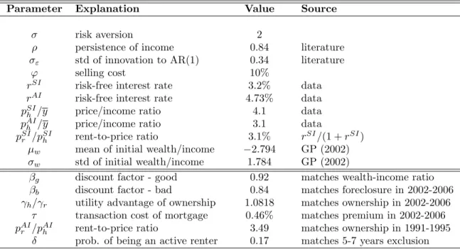
to match the homeownership rate in the 1991-1995 period using the interest rate and house price in that period. Table 1.2 presents the results of the calibration.
Table 1.2: Calibration
Parameter Explanation Value Source
σ risk aversion 2
ρ persistence of income 0.84 literature
σε std of innovation to AR(1) 0.34 literature
ϕ selling cost 10%
rSI risk-free interest rate 3.2% data
rAI risk-free interest rate 4.73% data
pSIh /y price/income ratio 4.1 data
pAIh /y price/income ratio 3.1 data
pSIr /pSIh rent-to-price ratio 3.1% r
SI/(1 +rSI)
µw mean of initial wealth/income −2.794 GP (2002)
σw std of initial wealth/income 1.784 GP (2002)
βg discount factor - good 0.92 matches wealth-income ratio
βb discount factor - bad 0.84 matches foreclosure in 2002-2006
γh/γr utility advantage of ownership 1.0818 matches ownership in 2002-2006
τ transaction cost of mortgage 0.46% matches premium in 2002-2006
pAIr /pAIh rent-to-price ratio 3.49 matches ownership in 1991-1995
Households. A model period is 1 year and households live for 65 periods. The mandatory retirement age is 45. Utility function for the households is the standard CRRA utility function with a slight modification to account for the benefit of homeownership: uk(c) = (γkc)
1−σ
1−σ , k ∈ {r, h} and γk is the utility advantage of
being a renter (k=r) or homeowner (k=h)19. I normalizeγr = 1, and calibrateγh
to match the homeownership rate in the 2002-2006 period. This impliesγh= 1.0818,
which means being a homeowner gives 8.18% more consumption than being a renter. I set the risk-aversion parameter, σ, to 2. I assume the measure of the good types,
µ, is 80%. The discount factor for the good type,βg, is fixed to 0.92 and for the bad type, it is calibrated to match the foreclosure rate in the 2002-2006 period. This gives me βb = 0.84.
For the income process before retirement, I take the parameters to be consis-tent with the findings of Hubbard, Skinner and Zeldes (1994), Carroll and Samwick (1997) and Storesletten, Telmer and Yaron (2004). Using their income process, I simulate an economy for a sufficiently long time and estimate the resulting income profile as an AR(1) process20. This gives us the income persistency, ρ, as 0.84 and standard deviation of the innovation to the AR(1) process, σε, as 0.34. I
ap-19
Given this utility specification, since there is no housing tenure choice and uncertainty after retirement, I can solve the value function at the time of retirement analytically: W(wr, yr) =
ur(¯c)1−κ
J−Jr+1
1−κ , wherewris the total wealth, including real estate, at the of retirement andyris
the retirement income level, ¯c= α1yr
α2 + wr α2,α1= 1−ωJ1−Jr+1 1−ω1 ,α2 = 1−ω2J−Jr+1 1−ω2 ,ω1 = (β(1+r))1/σ 1+r , ω2= 1+1r, andκ=β(β(1 +r)) 1−σ σ . 20
More specifically, I assume the stochastic component of the log income as a combination of an AR(1) component and transitory component. Within the range of these papers, I assume the persistency of the AR(1) process as 0.96, the standard deviation of the innovation to the AR(1) process as 0.16, and the standard deviation of the transitory shock as 0.22.
proximate this income process with a 15-states first-order Markov process using the discretization method outlined in Adda and Cooper (2003)21. For after retirement income, I assume λ = 0.35 and η = 0.2, meaning the retiree receives 35% of the income at the time of retirement plus 20% of the mean income in the economy. The probability of becoming an active renter, while the household is an inactive renter, is set to 0.17, to capture the fact that the bad credit flag stays approximately 5-7 years in the credit history of the household. The loss in the selling price of the house is set to ϕ = 10%22. The initial distribution of the income is assumed to be the stationary distribution. Following Gourinchas and Parker (2002), the initial distribution of the wealth to income ratio is assumed to be lognormal with mean
µw/y =−2.794 and standard deviationσw/y = 1.784.
Lenders. The annual risk-free interest rate is set torSI = 3.2% for the SI economy, which is the average real return on AAA corporate bond in the 2002-2006 period. The same rate is 4.73% in the 1991-1995 period. So, I set the risk-free interest rate in the AI economy to rAI = 4.73%. The annual transaction cost of mortgages to the lender is calibrated to match the mortgage premium in the 2002-2006 period. This gives me τ = 0.46% of the loan amount.
21
This approximation gives biased results as the persistency of the income process increases. To avoid this bias, I checked the accuracy of the approximation with 15-states Markov process and found that during computation settingρ= 0.85 andσε= 0.33 results the desired persistency and
standard deviation.
22Gruber and Martin (2003) estimates this cost for the homeowner as 7% using CEX data. Note
that I abstract from various other sources of selling the house like house price change, unemployment shock, medical expense shock and I also exclude the depreciation on the houses. So, I think 10% is a reasonable estimate of the transaction cost for selling the house.
Prices. For house prices, I use the metropolitan affordability index from Joint Center for Housing Studies. This index shows the median house price to median household income ratio. The ratio is 4.1 for the 2002-2006 period and 3.1 for the 1991-1995 period. So, I set the ratio of house price to mean income to
pSI r
y = 4.1 in the SI economy and pAI
h
y = 4.1 in the AI economy. Finally, rent-to-price
ratio,pSIr
pSIh is set to rSI
1+rSI = 3.1% in the SI economy23. For the AI economy, I calibrate
this ratio to match the homeownership rate in the 1991-1995 period. This gives me
pAI r pAI h = 3.49% 1.4.2 Results
I want to see whether the improvements in information technology - specif-ically the emergence of automated underwriting systems - can explain the recent changes in the mortgage market, particularly the decrease in the downpayment fraction and the increase in the mortgage premium, foreclosure rate, homeowner-ship rate, loan-to-value ratio, debt-service ratio, and dispersion of mortgage interest rates and downpayment fractions. To pursue this goal, given the above set of pa-rameters, I first solve the SI economy, which is my benchmark economy, and then compare the results to the AI economy. The AI economy represents the period before the introduction of automated underwriting systems, and the SI economy represents the period after the introduction of automated underwriting systems. These two pe-riods not only differ from each other in terms of information structure but also in
23
In the literature the imputed rent is calculated as the sum of cost of foregone interest, cost of property tax, maintenance cost, tax deductability of mortgage interest and expected capital gain. Since I abstract from all other dimensions, the imputed rent in my model corresponds to the cost of foregone interest, which is r