Graph-Optimization base multi-sensor fusion for robust UAV pose estimation

(1)

Graph-Optimization Based Multi-Sensor

Fusion for Robust UAV Pose Estimation

Master’s Thesis Final Report

Author:

Ruben Mascaró Palliser

Supervisors:

Lucas Pinto Teixeira

Timo Hinzmann

Prof. Dr. Margarita Chli

September 2017

(2)

(3)

Graph-Optimization Based Multi-Sensor Fusion for Robust UAV Pose

Estimation

Ruben Mascaro

1

_{, Lucas Teixeira}

1

_{, Timo Hinzmann}

2

_{, Roland Siegwart}

2

_{and Margarita Chli}

1 1

_{Vision for Robotics Lab, ETH Zurich, Switzerland}

2

_{Autonomous Systems Lab, ETH Zurich, Switzerland}

Abstract— Achieving accurate, high-rate pose estimates from proprioceptive and/or exteroceptive measurements is the first step in the development of navigation algorithms for agile mobile robots such as Unmanned Aerial Vehicles (UAVs). In this paper, we propose a decoupled multi-sensor fusion approach that allows the combination of generic 6D visual-inertial (VI) odometry poses and 3D globally referenced positions to infer the global 6D pose of the robot in real-time. Our approach casts the fusion as a real-time alignment problem between the local base frame of the VI odometry and the global base frame. The quasi-constant alignment transformation that relates these coordinate systems is continuously updated employing graph-based optimization with a sliding window. We evaluate the presented pose estimation method on both simulated data and large outdoor experiments using a small UAV that is capable to run our system onboard. Results are compared against different state-of-the-art sensor fusion frameworks, revealing that the proposed approach is substantially more accurate than other decoupled fusion strategies. We also demonstrate comparable results in relation with a finely tuned Extended Kalman Filter that fuses visual, inertial and GPS measurements in a coupled way and show that our approach is generic enough to deal with different input sources in a straightforward manner, as well as able to run in real-time.

I. INTRODUCTION

Navigation and control of Unmanned Aerial Vehicles (UAVs) requires precise and timely knowledge of the six degree-of-freedom robot pose (position and orientation) within space at any time. Though a plethora of systems and algorithms have been proposed in the past to address robot pose estimation, they are usually tailored to a single input source or to a very specific sensor suite. This makes them very sensitive to individual sensor failure modes and do not guarantee 100% availability necessary in real-world conditions.

As a result, literature has turned to more sophisticated approaches for multi-sensor data fusion. In this context, re-cent advances in robot state estimation combining cues from cameras and Inertial Measurement Units (IMU) have shown promising results for enabling robots to operate in mostly unstructured scenarios [1], [2]. However, these Visual-Inertial (VI) odometry algorithms accumulate errors in position and heading over time due to sensor noise and modelling errors. While the effect of such drift might be insignificant for small

This research was supported by the Swiss National Science Foundation (SNSF, Agreement no. PP00P2 157585) and EC’s Horizon 2020 Programme under grant agreement n. 644128 (AEROWORKS).

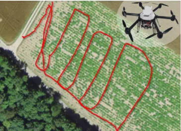
Fig. 1: The top view of the environment where the experiments presented in this paper were carried out. The red line represents the trajectory of one of the performed flights. The platform used is the AscTec Neo hexacopter, shown in the inset.

trajectories, reliable large-distance operation requires com-plementing VI odometry with localization measurements in a global reference frame. As in most state-of-the-art robotics systems, in this work we address this problem using global position measurements, such as GPS, to introduce globally referenced information into the proposed pose estimation framework.

VI odometry and global pose sources offer complemen-tary properties, which make them particularly suitable for fusion. On the one hand, VI odometry measurements are usually available at high frequencies, locally smooth and do not require previous knowledge about the environment. However, as aforementioned, these accumulate drift with growing distance from the starting point and they are not globally referenced (only an estimate of the robot pose with respect to the starting point of the trajectory is supported). On the other hand, estimates from global pose sources are globally referenced and their error is independent of the travelled distance. However, they are usually available at low frequencies, provide more noisy pose estimates and require previous knowledge (reference maps) or artificial modifica-tion (satellite placement, need of ground stamodifica-tions, etc.) of the environment. Combining both types of measurements in a graph-based multi-sensor fusion framework, our goal here is to estimate a trajectory, which is locally smooth and globally referenced at the same time.

(4)

In this paper, we present an approach for multi-sensor data fusion that decouples pose estimation from sensor fusion and can be executed online and in real-time. Pose estimation is formulated as a base frame alignment problem between local frame of the VI odometry and the global coordinate frame. The estimation of the transformation that relates both reference frames is continuously updated by running a sliding window graph-based optimization, leading to the maximum likelihood estimate over the joint probability distribution of robot poses in the current window. Our framework deals with multi-rate, generic sources, non-constant input frequencies and time-varying latencies in a simple and effective manner.

In brief, the main contributions of this paper are:

• a novel, efficient and accurate localization system based on the fusion of generic VI odometry 6D pose and global 3D position inputs,

• a novel graph construction strategy that is especially designed to achieve reliable global orientation estimates when only 3D global position measurements are avail-able,

• an evaluation of the system’s performance in both simulated and large outdoor flights over 1km, and

• demonstrated improvement of 1.5x to 3x in pose

estima-tion accuracy when comparing our approach with two of the most popular state-of-the-art VI-SLAM systems.

II. RELATED WORK

Most multi-sensor data fusion for navigation systems that currently appear in the literature can be categorised into filtering-based or smoothing approaches.

Conventional filtering-based approaches usually employ some variant of the Kalman filter. For example, in the context of small UAVs, Weisset al.[3] propose an Extended Kalman Filter (EKF) to fuse inertial measurements with GPS data and a camera-based pose estimate. Their work is generalized by Lynenet al.[4] to a modular multi-sensor fusion framework based on the iterated EKF formulation. In both cases, the propagation step is driven by high frequency inertial mea-surements, making the IMU an indispensable sensor on the system, and a lot of effort is put to align all other, potentially delayed, sensor readings with the states. With the same goal of achieving precise knowledge of position and orientation, especially in highly dynamic operation of robots, Bloeschet al.[1] propose an EKF-based VI odometry framework able to correct its pose estimate by integrating external pose updates, such as GPS measurements. Though all of these works report satisfactory results, the filtering-based approaches have in common that they restrict the state vector to the most recent state, hence marginalizing all older information, and it is mainly due to this reason that they perform suboptimally when compared to smoothing, as revealed in [5].

In contrast to filtering techniques, smoothing approaches formulate sensor fusion as a graph-based nonlinear least squares optimization problem. Using all past measurements up to the current one and optimizing the entire trajectory is commonly referred to as online batch estimation. This leads to a maximum likelihood estimate over the joint

probability of robot poses and produces statistically optimal results. Despite that incremental smoothing techniques, such as iSAM2 [6], are able to keep the problem computationally tractable, an important drawback of this approach lies with the fact that the full state vector is kept in memory over the entire trajectory, thus limiting its applicability to systems without memory constraints or having short operation times. An alternative to incremental smoothing techniques are the so-called sliding window filters, which keep the size of the state vector bounded by marginalizing out older states. In this context, Rehder et al. [7] propose a sliding window graph-based approach capable of localizing a vehicle in the global coordinate frame by using inertial measurements, long range visual odometry and sparse GPS information. Similarly, Merfels and Stachniss [8], [9] use a sliding window pose graph to fuse multiple odometry and global pose sources for self-localization of autonomous cars. The method that we present in this paper is closest to these approaches in the sense that it treats the fusion problem as a non linear optimization over a history robot poses with a graphical representation. However, after each optimization cycle we do not directly output the most recent estimated state. Instead, following the methodology presented in [10] and [11], we use the optimal solution to infer a base frame transformation that constantly realigns the local base frame of the VI odometry with the global base frame. The advantage of the approach we present here, over [10] and [11], is its ability to achieve global localization without previous knowledge about the environment (e.g. a reference map).

With the proposed method, the global pose of the robot can be estimated whenever a VI odometry pose measurement becomes available by simply applying the transformation that aligns it with the global coordinates, thus introducing minimal delay with respect to the time that the measure-ment is acquired. Taking advantage of the fact that the VI odometry measurements tend to be locally precise (meaning that the transformation between the VI odometry and the global frames stays quasi-constant over short periods of time), the proposed framework allows reducing the frequency of the optimization cycles w.r.t. the output rate of pose estimation without significantly diminishing accuracy. This is not possible in most state-of-the-art graph-fusion systems [7], [8], [9], in which the required output frequency determines also the frequency of the optimization cycles.

III. METHODOLOGY

Similarly to [10] and [11], we formulate the global lo-calization task as a rigid base frame alignment problem between a local coordinate frame (VI odometry reference frame) and the global coordinate frame. In our case, this is addressed by posing a sliding window graph-based multi-sensor fusion problem that constantly seeks the most recent

N optimal, globally referenced, robot states. The solution of each optimization cycle is used to update the quasi-constant transformation between the local and the global base frames, thus allowing a smooth realignment of the VI odometry pose estimates to the global base frame.

(5)

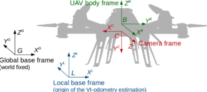
Fig. 2:The frame setup of our pose estimation system.

Figure 2 depicts the frame setup of our pose estimation system. Each frame is connected with a certain homogeneous transformationT to another frame. The global base frameG

is world fixed and serves as the origin for all global position measurements. The local base frame L forms the origin of the VI odometry pose estimates and is originally placed at the starting point of the trajectory. The body frame B is rigidly attached to the robot’s centre of mass and the camera frameC is centred in the respective sensor of the robot.

Based on visual and inertial information, the VI odometry estimates the transformation LTB between the local base frame L and the body frame B. For the purpose of this section, we assume that the transformation BTC between the body frame and the camera frame is calibrated online by the VI odometry. Additionally, a GPS sensor provides the 3D position of the body frame in global coordinates,

GpB. The final goal of the online localization is to estimate the transformation GTB in real-time. This transformation can also be expressed as the product of the quasi-constant transformation between the global and local base frames,

GTL, which is calibrated online by our multi-sensor fusion

framework, and the input VI odometry pose estimate,LTB.

Using this approach, we are able to output a globally refer-enced pose estimate each time a VI-odometry measurement is available and with minimal delay with respect to the time it is acquired. This allows us to decouple the output rate of the localization system from the frequency of the optimization cycles, as they are only used to update the transformation between the global and the local base frames, GTL. Since the VI odometry pose estimates are supposed to be locally precise, the frequency of the optimization cycles can be slightly lower than the output rate of the localization system without inducing considerable losses in accuracy. This way, we are able to achieve accurate, real-time global localization with less frequent optimization cycles than conventional approaches, which directly output the most recent optimal state each time a graph optimization is performed.

Below we describe each stage in the process of estimating the base frame transformation GTL by means of a sliding window graph-based multi-sensor fusion approach.

A. Time alignment of input data

Integrating input sources with unknown time behaviour is not straightforward as we have to deal with multi-rate sources, non-constant input frequencies and out-of-sequence

estimates. Similarly to [8] and [9], our approach consists in buffering all incoming data before the next graph construc-tion phase. Sorting the data by time allows integrating of out-of-sequence data in a natural way.

At the start of each cycle and in order to force a proper graph structure to solve the multi-sensor fusion problem, the buffered local and global measurements need to be time-aligned. To achieve that, we match each available global measurement with the VI odometry pose estimate that has the closest timestamp and we make them virtually point to a same instant in the past. This strategy is based on the assumption that the output rate of the VI odometry is much higher than the output rate of the GPS sensor. As detailed in section IV, we design a specific experimental setup, in which the VI odometry pose estimates and the GPS readings are provided at frequencies of 100Hz and 5Hz, respectively, meaning that the maximum expected delay between matched measurements is 5ms.

B. Graph construction

Our approach to multi-sensor fusion consists in construct-ing and solvconstruct-ing a nonlinear optimization problem over a limited history of sensor measurements and robot states that can be represented as a sliding window pose graph. The graph consists of a set of nodes that represent past, globally referenced robot poses at discrete points in time. Sensor measurements induce constraints on these robot poses and are modelled as edges connecting the nodes of the graph.

In contrast to related graph-based approaches [7], [8], [9], we do not generate a node every time a VI odometry pose estimate is available nor tie its generation to a specific time step, which requires lots of interpolations between measurements [8]. Instead, we generate a new node only when a pair of time-aligned local and global measurements is found. By doing this, we increase the temporal resolution of the graph, thus reducing both the number of nodes contained in each window and the time needed to solve the optimization problem.

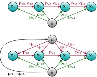
1) The conventional graph structure: A common way to construct the graph is to distinguish between local mea-surements (VI odometry), that induce edges between two successive nodes, and global measurements (GPS), which impose constraints on the position in a global coordinate frame. By introducing a virtual zero node G at the origin of the coordinate system into the graph (see Figure 3), both classes of constraints can be treated in a unified way [7]. However, as we demonstrate in section IV, if only 3D positions are available as global measurements, this approach is prone to yield wrong global orientation estimates.

2) Adding an extra virtual node to restrict orientations:

In order to constrain absolute orientation, Rehder et al. [7] employ accelerometers as inclinometers. Here, we propose to add a second virtual node L at the origin of the local coordinate system, which is constrained in the global coordi-nate frame by the current estimation of the rotation between the local and the global base frames. In this new approach, VI odometry measurements induce two types of constraints:

(6)

G x2 x1 x3 x4 pG1 pG2 pG3 pG4 p12,q12 p23,q23 p34,q34 L x2 x1 x3 x4 G pG1 pG2 pG3 pG4 p12 p23 p34 qL1 qL2 qL3qL4 pGL,qGL

Fig. 3:Comparison between the conventional graph structure (top) and the structure proposed in this paper (bottom). Green arrows represent the constraints generated by global position measure-ments, whereas magenta arrows represent the constraints generated by VI odometry pose estimates. Note that in our approach VI odometry measurements induce two types of constraints: position constraints between consecutive nodes and orientation constraints between each node and the virtual L node. The virtual L node tracks the orientation between the VI odometry local frame and the global reference frame, thus providing a prior to obtain reliable global orientation estimates.

orientation constraints between the virtualL node and each other node in the graph, and position constraints between consecutive nodes. A comparison between the conventional graph structure and the one that is proposed in this work is illustrated in Figure 3.

During each graph construction phase, the constraint relat-ing the virtualG andLnodes is updated with theLoptimal pose obtained in the previous optimization cycle, which stores the optimal rotation between the local and global base frames given the history of measurements contained in the sliding window. This strategy requires a method to initialize the mentioned constraint in the first graph con-struction phase. For that, we formulate a standard least-squares fitting problem between two sets of time aligned global and local 3D position measurements acquired during an initialization period. The solution, which can be obtained using the approach based on singular value decomposition proposed in [12], is the optimal transformation between the local and the global base frames after the initialization period and thus can be applied as a constraint between the virtual

G andLnodes in the first graph construction phase.

C. Graph optimization

Once the graph is built, optimizing it consists in finding the configuration of nodes that best fits all the available measurements, which are subjected to noise. We assume this noise to be additive, white and normally distributed with zero mean.

Our approach exploits the well-established graph-based Si-multaneous Localization and Mapping (SLAM) formulation [13], but applies it to the case of sensor data fusion. Let

x= (x1, ...,xm) T

be the state vector, where xi = (pi,qi)

describes the global pose of the node i, with pi being the

position and qi the orientation of the robot. Consider also

a set of measurements, withzij = (pij,qij)andΩij being

the mean and the information matrix, respectively, of a single measurement relating the nodeiand the nodej (we denote by pij and qij the translation and rotation both measured

from nodei to node j). The least squares estimation seeks the state x∗ that best explains all observations given the `2

norm. This is equivalent to solving the following equation:

x∗= argmin

x

X

hi,ji∈C

eT_ijΩijeij, (1)

where C denotes the set of pairs of indices, for which a measurement is available andeij =e(xi,xj,zij)is a vector

error function that measures how well the constraint from the measurementzijis satisfied. In our case, the information

matricesΩij are the inverses of the measurement covariance

matrices. Additionally, in order to increase the robustness against outliers, we apply the Pseudo-Huber cost function to all constraints.

The solution of (1) can be found by linearising the equation around an initial guessxˇ, which leads to iteratively solving a linear system with the system matrix H and the right-hand side vectorbsuch that

H= X hi,ji∈C Jij(ˇx) T ΩijJij(ˇx), (2) bT = X hi,ji∈C eT_ijΩijJij(ˇx), (3)

whereJij(xˇ)is the Jacobian of the error function computed

in ˇx. For a more detailed explanation, we refer the reader to [13]. To effectively solve the non-linear optimization problem, we use the Google Ceres Solver [14].

D. Base frame transformation estimation

After each optimization cycle, instead of sending out the most recent optimal robot pose, we perform an additional step that realigns the VI odometry frame to the global coor-dinate frame. The transformation between the VI odometry and the global coordinate frames is captured by estimation of a base frame transformation GTL that can be expressed as

GTL =GTB·LTB−1, (4)

where GTB denotes the most recent optimal, globally ref-erenced robot pose and LTB is the VI odometry local pose estimate that is time-aligned with this most recent state.

In a practical sense, the quasi-constant base frame trans-formationGTL captures the unobserved global position and

orientation and the drift of the VI odometry. By running the optimization cycles at a sufficiently high frequency, our approach provides a way to realign the VI odometry pose estimates with the global reference frame and correct the mentioned drift in a smooth way.

(7)

E. Graph update

At the beginning of a new graph construction phase, we generate as many new nodes as the number of global measurements acquired during the previous cycle. To keep the size of the graph constant, we simply discard older nodes that do not lay inside the sliding window at the current time. The virtual nodes G and L are always maintained in the graph.

After adding the new nodes into the graph, the time-aligned local and global measurements received in the previ-ous cycle are mapped as edges between them. Additionally, the constraint relating the virtual nodesG andL is updated with theL optimal transformation obtained in the previous cycle. Finally, the optimal poses obtained in the previous cycle are used as initial guess in the new optimization problem. This leads to an effective and efficient solution in practice as very few optimization steps are usually sufficient to integrate the new information of the current time step.

IV. EVALUATION

This section presents our experimental evaluation of the proposed framework. We first introduce a brief description of the pose estimation system that has been used in this work and then we evaluate the performance of our algorithm on both simulated and real data.

A. Overview of the pose estimation system

Figure 4 shows the online pose estimation system with which all the experiments presented in this paper have been conducted. In a first step, based on the information provided by a camera and an IMU mounted together on a single visual-inertial sensor attached to the UAV, the VI odometry estimates the pose of the camera in local coordinates. We test the performance of the system with both OKVIS [2], a keyframe-based VI odometry framework that uses nonlinear optimization, and ROVIO [1], an EKF-based VI odometry approach. Secondly, the Multi Sensor Fusion Framework [4] (MSF) fuses the camera pose from the VI odometry with the measurements acquired by the UAV’s IMU and estimates the pose of the UAV body frame in local coordinates. This is what we refer to as our VI odometry input in the following subsections. Finally, our GOMSF framework fuses the local UAV poses provided by MSF with GPS position measurements and estimates the pose of the UAV in global coordinates. We also run the pose estimation framework

Fig. 4:Overview of the proposed pose estimation system, which is referred to asGOMSF(OKVIS/ROVIO)in the following subsections.

Fig. 5:Overview of the sensor fusion approach based on the MSF EKF for global pose estimation, using ROVIO as VI odometry input. Experiments performed with this pose estimation framework are labelled asMSF(ROVIO)in the following subsections.

Fig. 6: Overview of the sensor fusion approach based on the ROVIO EKF for global pose estimation. Experiments performed with this pose estimation framework are labelled asROVIO+GPS in the following subsections.

using the conventional graph-based sensor fusion approach (CGSF) showed in Figure 3 to demonstrate the benefits of adding the virtual L node in the graph, as proposed in this paper. The overall system runs in real time at the frequencies detailed in Figure 4.

To test the accuracy of the proposed system, we compare our results against the solution obtained with two state-of-the-art, filtering-based sensor fusion strategies: the first one consists in fusing the UAV’s IMU measurements, the VI odometry pose estimates and the GPS readings together in the MSF, as proposed in [3], whereas the second one consists in integrating the GPS position updates directly into ROVIO and fusing its output with the UAV’s IMU readings by means of the MSF, as presented in [15]. Diagrams of these alternative approaches are shown in Figures 5 and 6, respectively.

B. Experiments with synthetic input data

The following experiments are designed to show that the proposed multi-sensor fusion framework is able to effectively estimate the global 6D pose of the UAV given a set of locally referenced 6D poses and 3D global positions. We also demonstrate that adding the virtualLnode in the graph notably increases accuracy.

To carry out the experiments, we use inertial data and exact 6D ground truth extracted from simulated flights generated with the gazebo simulator1_{. Visual data is created in blender}2

by exporting the simulated trajectories into a virtual 3D scenario. Finally, global position estimates are generated at

1_{http://gazebosim.org} 2_{https://www.blender.org}

(8)

Fig. 7:The virtual scenario used to generate visual data.

runtime with a frequency of 5Hz by adding Gaussian noise to the ground truth positions.

We evaluate the online pose estimation on five different simulated flights performed with the camera pointing forward and over the same virtual scenario: a mining quarry (Figure 7) of approximately 250m × 200m. In all of these experi-ments we run OKVIS to get the VI odometry pose estimates. The standard deviation of the noise used to generate the global position estimates is 0.5m in the X and Y axes and 0.75m in the Z axis.

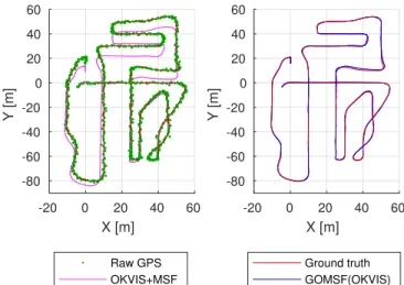
An example of our framework’s input and output data corresponding to flight 2 is shown in Figure 8. As explained above, our inputs are noisy GPS 3D position measurements and VI odometry 6D pose estimates that accumulate drift with the travelled distance. The output of GOMSF is a set of globally referenced poses that follow the ground truth closely, providing more accuracy and smoothness than the simulated GPS raw measurements, while diminishing the VI odometry drift effects.

Figures 9 and 10 illustrate the temporal evolution of the position and orientation errors obtained when running GOMSF in flight 2. Additionally, we plot the errors that are obtained using the conventional graph-based sensor fusion strategy (CGSF), that is, representing the 6D pose

mea--20 0 20 40 60 X [m] -80 -60 -40 -20 0 20 40 60 Y [m] Raw GPS OKVIS+MSF -20 0 20 40 60 X [m] -80 -60 -40 -20 0 20 40 60 Y [m] Ground truth GOMSF(OKVIS)

Fig. 8: Input data (left) and estimated global trajectory (right) compared against exact ground truth for flight no. 2. Note that VI-odometry pose estimates (obtained by running OKVIS and MSF) have been aligned with the ground truth at the beginning of the trajectory to facilitate the visualization of the drift.

30 60 90 120 150 180 time [s] -2 0 2 X error [m] 30 60 90 120 150 180 time [s] -4 -2 0 Y error [m] 30 60 90 120 150 180 time [s] -4 -2 0 2 4 Z error [m] Raw GPS CGSF(OKVIS) GOMSF(OKVIS)

Fig. 9:Comparison between the position errors obtained using the conventional graph structure (noLnode) and our approach in flight 2. Also GPS position errors are plotted to provide an insight of how noisy GPS measurements are.

30 60 90 120 150 180 time [s] 10-2 100 102 error [ ° ] 30 60 90 120 150 180 time [s] 10-2 100 102 error [ ° ] 30 60 90 120 150 180 time [s] 10-2 100 102 error [ ° ] CGSF(OKVIS) GOMSF(OKVIS)

Fig. 10:Comparison between the orientation errors obtained using the conventional graph structure (noLnode) and our approach in flight 2. Orientation errors are expressed using the roll-pitch-yaw (φ,θ,ψ) convention.

surements as constraints between successive nodes without adding the virtualL node in the graph (see Figure 3). Note that, in the latter case, we obtain frequent wrong orientation estimates that also induce significant errors in the estimate of the robot global position.

(9)

Flight 1 2 3 4 5 Travelled dist. [m] 765.5 737.6 850.9 758.4 996.6 mean X error [m] 0.15 0.14 0.21 0.28 0.16 std X error [m] 0.11 0.13 0.18 0.18 0.13 mean Y error [m] 0.23 0.37 0.25 0.20 0.35 std Y error [m] 0.18 0.36 0.23 0.19 0.27 mean Z error [m] 0.13 0.15 0.14 0.14 0.14 std Z error [m] 0.10 0.12 0.11 0.10 0.11 meanφerror [◦] 0.35 0.53 0.38 1.50 0.44 stdφerror [◦] 0.30 0.37 0.29 0.67 0.64 meanθerror [◦] 0.86 0.95 0.40 1.18 0.90 stdθerror [◦] 0.34 0.49 0.26 0.91 0.90 meanψerror [◦] 1.19 1.18 1.41 2.53 7.72 stdψerror [◦] 0.57 0.74 0.95 1.74 6.16

TABLE I: Mean and standard deviation of the absolute position and orientation (roll-pitch-yaw) errors in all five evaluated flights using GOMSF(OKVIS). A sliding window containing the 25 most recent robot states and updated each 0.3 s is used in all experiments.

Analysing the performance of GOMSF on all five tra-jectories (Table I), we can see that the mean translation error lies below 0.4 m in all three axes. Orientations are estimated with a mean error which is below 1.5◦ in most cases except in flights 4 and 5, corresponding to zig-zag trajectories, where bigger errors in the yaw angle estimates are obtained. With the approach we propose in this paper, the output of the sensor fusion framework improves compared to the individual input sources in all simulated flights (the mean errors of the GPS raw measurements are approximately 0.4m in the X and Y axes and 0.6m in the Z axis).

C. Experiments in large outdoor flights

The following experiments are conducted on real input data and are designed to test the generality of GOMSF in dealing with different VI odometry systems and its ability to run online on a UAV in comparison to the state-of-the-art sensor fusion approaches.

In this case, we present the results obtained with three datasets that were recorded in previous work [11] by per-forming flights over a vegetable field of 100m × 60m with the camera pointing downwards. A top view of the environment and a representation of the trajectory performed in flight 3 is shown in Figure 1. The visual-inertial data was collected with the VI-Sensor [16], which is equipped with two WVGA monochrome cameras running at 20Hz and an ADIS 16448 MEMS IMU running at 200Hz. Body-referenced inertial and global position measurements were acquired by the on-board IMU (200Hz) and GPS (5Hz) modules of the AscTec Neo hexacopter, carrying the VI-Sensor. Finally, accurate ground truth 3D positions were acquired using a Leica Nova TM50 ground station, which is able to track a prism mounted on the UAV with sub-centimetre accuracy.

For each dataset, we run GOMSF to fuse the GPS mea-surements with OKVIS or ROVIO (see Figure 4). We also run the framework using the conventional graph-based sensor fusion strategy (CGSF) showed in Figure 3 to demonstrate that our approach, which adds the virtual L node in the graph, leads to better accuracy. Additionally, we compare

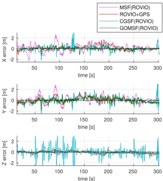
50 100 150 200 250 300 time [s] -2 0 2 X error [m] 50 100 150 200 250 300 time [s] -2 0 2 Y error [m] 50 100 150 200 250 300 time [s] -2 0 2 Z error [m] MSF(ROVIO) ROVIO+GPS CGSF(ROVIO) GOMSF(ROVIO)

Fig. 11: Temporal evolution of the position errors obtained with four different sensor fusion systems on dataset 3 of [11].

GOMSF’s performance against the setup of Figure 5 to fuse ROVIO, GPS and the UAV’s IMU in the MSF and the setup of Figure 6 to integrate the GPS position updates directly into ROVIO. In all cases, we evaluate the results against the Leica ground truth positions (note that we have no way of capturing orientation ground truth in the real experiments).

Figure 11 shows the temporal evolution of the position errors obtained when running all systems using ROVIO for VI odometry on the longest trajectory, which corresponds to flight 3. A detailed analysis of the mean and the standard deviation of the absolute translation errors obtained in all experiments with the tested datasets is provided in Table II.

Though all compared localization systems are able to provide globally referenced position estimates, results vary from one approach to another. In all tested datasets, the lowest mean translation errors are achieved with our graph-optimization based sensor fusion approach, specially when OKVIS is used for VI odometry. However, the most interest-ing interpretation of the results derives from the comparison between the experiments performed with ROVIO, which show that, using the same inputs, our algorithm achieves more accurate pose estimates than the two EKF-based ap-proaches. With a generic method for fusing 6D locally refer-enced pose estimates and 3D global position measurements, we not only outperform the generic MSF framework, but also ROVIO, which was specifically designed to fuse visual-inertial data with external position updates. This reinforces the findings of [5], that non-linear optimization is preferable to filtering-based methods.

Following this experimental analysis, we observe that any errors arising with GOMSF during online pose estimation are mainly obtained in regions where the drift of the VI odometry

(10)

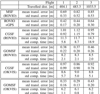
Flight 1 2 3 Travelled dist. [m] 404.1 483.3 1033.5 MSF

(ROVIO)

mean transl. error [m] 0.69 0.82 0.85 std transl. error [m] 0.33 0.52 0.53 ROVIO

+GPS

mean transl. error [m] 0.42 0.44 0.64 std transl. error [m] 0.17 0.20 0.30 CGSF

(ROVIO)

mean transl. error [m] 1.01 1.12 0.95 std transl. error [m] 0.92 1.15 0.79 mean comp. time [ms] 11.3 11.7 14.3 std comp. time [ms] 5.8 8.7 18.9 GOMSF

(ROVIO)

mean transl. error [m] 0.38 0.37 0.46 std transl. error [m] 0.22 0.20 0.26 mean comp. time [ms] 8.2 8.3 8.5

std comp. time [ms] 2.1 2.1 2.0 CGSF

(OKVIS)

std comp. time [ms] 5.7 5.0 5.1 GOMSF

(OKVIS)

std comp. time [ms] 1.1 0.8 1.0

TABLE II:Mean and standard deviation of the absolute translation errors for all experiments in the three evaluated flights. Also the mean and the standard deviation of the computation time, which comprises the time needed to build and solve a graph-optimization problem, is included in the experiments in which GOMSF and CGSF are used.

increases substantially within a short interval of time. This issue appears quite frequently when running ROVIO with the datasets presented here, and it is mainly due to this reason that the performance of GOMSF is better when paired with OKVIS instead of ROVIO. This implies that our online pose estimation could still be improved with a strategy to detect such fast drifting modes of the VI odometry early and decrease the corresponding weights during optimization.

In Table II, for the experiments in which the graph-based sensor fusion approaches (GOMSF and CGSF) are run, we also include the mean and the standard deviation of the time needed for constructing and optimizing the graph in each cycle, which we sum up as computation time. All GOMSF and CGSF experiments shown here have been performed using a sliding window with the 25 most recent UAV states (nodes) and running a new optimization cycle each 0.25 seconds (approximately each time a new GPS measurement is available). Note that, for this sliding window size, the GOMSF’s mean computation time is lower than 10ms (i.e. more than 20 times smaller than the period of the optimization cycles) in all experiments, which ensures a consistent behaviour of the framework.

V. CONCLUSIONS

The multi-sensor fusion approach GOMSF presented in this paper is motivated by the need of accurate, high-rate pose estimates during long-term operations performed with UAVs in unstructured outdoor environments. We fulfil these requirements by proposing a sliding window graph-based optimization scheme that continuously realigns the odometry pose estimates with the global reference frame. Furthermore, we describe a particular graph structure that allows us to

obtain reliable global orientation estimates given only 3D globally referenced positions.

The proposed system is first evaluated on simulated flights revealing its ability to infer reliable global position and orientation estimates. Tests on real outdoor flights against popular state-of-the-art VI-SLAM approaches reveal consis-tently more robust and accurate performance of GOMSF, especially when the system runs together with a key-frame based VI odometry framework (OKVIS).

Future directions will focus on detecting significant drift in the VI odometry pose estimates and account for this during optimization.

REFERENCES

[1] M. Bloesch, S. Omari, M. Hutter, and R. Siegwart, “Robust Visual Inertial Odometry Using a Direct EKF-Based Approach,” in Proceed-ings of the IEEE/RSJ International Conference on Intelligent Robots and Systems (IROS), 2015.

[2] S. Leutenegger, S. Lynen, M. Bosse, R. Siegwart, and P. Furgale, “Keyframe-based visual inertial odometry using nonlinear optimiza-tion,”The International Journal of Robotics Research (IJRR), vol. 34, no. 3, pp. 314 – 334, 2015.

[3] S. Weiss, M. W. Achtelik, M.Chli, and R.Siegwart, “Versatile Dis-tributed Pose Estimation and Sensor Self-Calibration for an Au-tonomous MAV,” inProceedings of the IEEE International Conference on Robotics and Automation (ICRA), 2012.

[4] S. Lynen, M. W. Achtelik, S. Weiss, M. Chli, and R. Siegwart, “A Robust and Modular Multi-Sensor Fusion Approach Applied to MAV Navigation,” inProceedings of the IEEE/RSJ International Conference on Intelligent Robots and Systems (IROS), 2013.

[5] H. Strasdat, J. Montiel, and A. J. Davison, “Visual SLAM: Why filter?” Image and Vision Computing, vol. 30, no. 2, pp. 65–77, 2012. [6] M. Kaess, H. Johannsson, R. Roberts, V. Ila, J. Leonard, and F.

Del-laert, “iSAM2: Incremental Smoothing and Mapping Using the Bayes Tree,” International Journal of Robotics Research (IJRR), vol. 31, no. 2, pp. 217–236, 2012.

[7] J. Rehder, K. Gupta, S. Nuske, and S.Singh, “Global Pose Estimation with Limited GPS and Long Range Visual Odometry,” inProceedings of the IEEE International Conference on Robotics and Automation (ICRA), 2012.

[8] C. Merfels and C. Stachniss, “Pose Fusion with Chain Pose Graphs for Automated Driving,” inProceedings of the IEEE/RSJ International Conference on Intelligent Robots and Systems (IROS), 2016. [9] C. Merfels and C. Stachniss, “Sensor Fusion for Self-Localisation of

Automated Vehicles,” Journal of Photogrammetry, Remote Sensing and Geoinformation Science (PFG), vol. 85, no. 2, pp. 113–126, 2017. [10] H. Oleynikova, M. Burri, S. Lynen, and R. Siegwart, “Real-Time Visual-Inertial Localization for Aerial and Ground Robots,” in Pro-ceedings of the IEEE/RSJ International Conference on Intelligent Robots and Systems (IROS), 2015.

[11] J. Surber, L. Teixeira, and M. Chli, “Robust Visual-Inertial Localiza-tion with weak GPS priors for Repetitive UAV Flights,” inProceedings of the IEEE International Conference on Robotics and Automation (ICRA), 2017.

[12] K. S. Arun, T. S. Huang, and S. D. Blostein, “Least-Squares Fitting of Two 3-D Point Sets,”IEEE Transactions on Pattern Analysis and Machine Intelligence, vol. 9, no. 5, pp. 698–700, 1987.

[13] G. Grisetti, R. Kmmerle, C. Stachniss, and W. Burgard, “A Tutorial on Graph-Based SLAM,” IEEE Intelligent Transportation Systems Magazine, vol. 2, no. 4, pp. 31–43, 2010.

[14] S. Agarwal, K. Mierle,et al.Ceres Solver. http://ceres-solver.org. [15] R. Bhnemann, D. Schindler, M. Kamel, R. Siegwart, and J. Nieto,

“A Decentralized Multi-Agent Unmanned Aerial System to Search, Pick Up, and Relocate Objects,” inIEEE International Symposium on Safety, Security, and Rescue Robotics (SSRR), 2017.

[16] J. Nikolic, J. Rehder, M. Burri, P. Gohl, S. Leutenegger, P. Furgale, and R. Siegwart, “A Synchronized Visual-Inertial Sensor System with FPGA Pre-Processing for Accurate Real-Time SLAM,” inProceedings of the IEEE International Conference on Robotics and Automation (ICRA), 2014.

(11)

Contact

Vision for Robotics Lab LEE H

IRIS, D-MAVT, ETH Zurich Leonhardstrasse 21 CH-8092 Zurich Switzerland

www.v4rl.ethz.ch