Vol. 5, No. 1, February 2019 ISSN 2374-2410 E-ISSN 2374-2429 Published by Redfame Publishing URL: http://afa.redfame.com
Rating Migration and Bond Valuation: Towards Ahistorical Rating
Migration Matrices and Default Probability Term Structures
Brian BarnardCorrespondence: Brian Barnard, Wits Business School, University of the Witwatersrand (WITS), South Africa. Received: January 17, 2017 Accepted: December 14, 2018 Available online: January 16, 2019 doi:10.11114/afa.v5i1.2157 URL: https://doi.org/10.11114/afa.v5i1.2157
Abstract
The study examines rating migration, and default probability term structures obtained from rating migration matrices. It expands on the use of rating migration matrices with reduced form bond valuation models, by formally delineating the probability of default according to the likely rating paths of a bond, as implied by the rating migration matrix. Further, two alternatives are also considered. First, the cost of default is stipulated as the recovery of par according to the exit rating upon default. Also, in addition to stating the value of a bond in terms of expected cash flows, when considering the probability of default, the value of a bond is alternatively stated as the present value of all likely rating paths of the bond, discounted against the market risk-bearing bond forward rates of the different rating categories. The impact of term structure volatility and rating migration uncertainty on bond valuation is also considered.
It is shown that the relationship between rating migration and default probability is complex, and the default probabilities of different rating categories are time-dependent and not isolated from each other. Also, rating migration resembles a delayed default process that influences default probabilities of subsequent intervals. The implications of a rating migration matrix may perhaps only be fully understood through simulation. This form one of the first points by which to evaluate rating migration matrices. The results of the valuation model show that historical rating migration matrices may not be optimal for pricing bonds ahistorically. A principal premise of the study is the dichotomy between historical values and ahistorical estimates, particularly with regards to rating migration. It is argued that historical estimates face two key shortcomings: they must be able to accurately forecast future rating migration and rating category intensities as a result, and they must specify a method to include rating migration uncertainty. An optimization model is delineated to extract ahistorical rating migration matrices from market prices. This too has implications that should be considered. In light of the above, reduced form models may have an advantage over structural models, in their ability to portray a far more sophisticated default process.
Keywords: default probability, default risk, credit risk, rating migration, bond valuation 1. Introduction
1.1 The Factors Impacting Bond Valuation
Huang and Huang (2012) find that, for investment grade bonds (those with a credit rating not lower than Baa) of all maturities, credit risk accounts for only a small fraction - typically around 20%, and, for Baa-rated 10-year bonds, in the 30% range - of the observed corporate-Treasury yield spreads, and it accounts for a lower fraction of the observed spreads for bonds of shorter maturities. For junk bonds, however, credit risk accounts for a much larger fraction of the observed corporate-Treasury yield spreads. Geske and Delianedis (2001) conclude that credit risk and credit spreads are not primarily explained by default and recovery risk, but are mainly attributable to taxes, jumps, liquidity, and market risk factors. Also, Elton et al (2001) reach a similar conclusion that credit spreads are not primarily explained by default and recovery risk.
Merton (1974) hypothesizes that the value of corporate debt is determined by the risk free rate, issue traits and default risk. Fama and French (1993) capture two factors specific to bonds. One common risk in bond returns arises from unexpected changes in interest rates - they proxy for the deviation of long-term bond returns from expected returns due to shifts in interest rates, and note that term-structure variables are likely to play a role in bond returns. The other stated factor is default risk. Whilst extensively modelling liquidity risk, Houweling et al (2005) note interest rate risk and credit risk as principal factors. Elton et al (2004) use a homogeneous group of bonds to minimize risk differences. They show that pricing errors within a group vary with bond characteristics. In particular, they consider default risk, liquidity,
tax liability, recovery rates, and age.
Grandes and Peter (2005) delineate a currency (risk) premium, a default (risk) premium, and a jurisdiction premium. They find that although firm-specific factors are significant in explaining the risk premium investors demand to hold corporate debt, a much more important part of this premium can be attributed to macroeconomic risk factors of the country in which a firm operates. According to them, the corporate default premium is a function of i) sovereign risk, ii) leverage, iii) firm-value volatility, iv) interest rate volatility, v) remaining time to maturity, and vi) liquidity. Contrasted with more specific credit risk, Delianedis and Geske (2003) delineate market risk as including equity risk, currency risk, interest rate risk, commodity price risk, and asset price risk.
Campbell and Taksler (2003) note equity volatility as factor - both idiosyncratic volatility and systematic or market-wide volatility. They conclude that firm specific equity volatility is an important determinant of the corporate bond spread and that the economic effects of volatility are large. They also suggest including a risk premium on systematic credit risk. Elton et al (2001) state default risk, taxes and systemic risk - compensation for the systematic nature of risk in bond returns. Collin‐Dufresne et al (2001) point to local supply-demand shocks that are independent of both changes in credit-risk and typical measures of liquidity. In particular, there seems to exist a systematic risk factor in the corporate bond market that is independent of equity markets, swap markets, and the Treasury market and that seems to drive most of the changes in credit spreads.
Athanassakos and Carayannopoulos (2001) see the factors that impact bond value as default risk, tax, specific issue traits, and short-run deviations from equilibrium. In turn, short-run deviations from equilibrium entails liquidity risk, the business and economic environment and conditions, and temporary imbalances of demand and supply between corporate and treasury bonds. The effects of economic conditions and the business cycle on yield spreads are captured with the use of three proxy variables: the annual rate of change in the consumer price index (inflation rate), the quarterly change in the difference between the 20-year and the three-month treasury yields, and the annual rate of change in industrial production index. In addition, whether maturity should be included as a factor is contested.
Elton et al (2001) argue that, if corporate bond returns move systematically with other assets in the market whereas government bonds do not, then corporate bond expected returns would require a risk premium to compensate for the non-diversifiability of corporate bond risk, just like any other asset. The literature of financial economics provides evidence that government bond returns are not sensitive to the influences driving stock returns. There are two reasons why changes in corporate spreads might be systematic. First, if expected default loss were to move with equity prices, so while stock prices rise default risk goes down and as stock prices fall default risk goes up, it would introduce a systematic factor. Second, the compensation for risk required in capital markets changes over time. If changes in the required compensation for risk affects both corporate bond and stock markets, then this would introduce a systematic influence. They believe the second reason to be the dominant influence. The Fama-French (1993) model employs the excess return on the market, the return on a portfolio of small stocks minus the return on a portfolio of large stocks (the SMB factor), and the return on a portfolio of high minus low book-to-market stocks (the HML factor) as its three factors. Das and Tufano (1995) state investors are exposed to three risks: interest rate risk, changes in credit risk caused by changes in the credit rating of the issuer of the debt, and changes in credit risk caused by changes in spreads on the debt, even when ratings have not changed. Altman (1996) examines the expected spread change and cost implication due to credit rating migration. In the context of portfolios, Fei et al (2012) note that risk models generally predict for each asset in the portfolio, the corresponding probability of default (PD), exposure at default (EAD) and loss given default (LGD). This is also referred to as credit rating migration risk, or simply credit migration risk. Similarly, Kadam and Lenk (2008) note different estimates for risk capital, derived from loss distributions, which they quantify as Value-at-Risk (VAR) and Expected Loss (EL) for the portfolio at hand. Jarrow et al (1997) model the impact in forward rates - and thus bond value - due to credit rating jumps.
Delianedis and Geske (2003) note that default probabilities and changes in expected default frequencies are important to both the structure and pricing of credit derivatives. All corporate issuers have some positive probability of default. This default probability should change continuously with changes in the firm’s stock price and thus its leverage. The value of most fixed income securities is typically inversely related to the probability of default. Investors are concerned about changes in the value of their fixed income securities due to changes in the probability of default, even though the actual default seldom occurs. In fact, fixed income investors may be more concerned with changes in the perceived credit quality of their bond holdings than with actual default. Rating migrations, which offer one reflection of changes in perceived quality of bonds, occur much more frequently than defaults.
Foss (1995) specifically differentiates between credit risk and default risk. He notes that the terms default risk and credit risk are often used interchangeably; however, they are not one and the same. Default risk is defined as the risk that the issuer of a fixed-income security will be unable to make timely payments of interest or principal. This risk, diversified over a portfolio of equally rated securities, leads to an expected default loss. Many of the initial studies on risks and
returns focus on historical default rates and losses. Although these studies provide valuable insight, default rates and default losses, in isolation, are not paramount. Credit risk is defined as the risk that the perceived credit quality of an issuer will change, although default is not necessarily a certain event. Increased credit risk is reflected in a widening of the yield spread. Credit and default risk are correlated because credit deterioration is almost always a precursor to eventual default; even in the most drastic cases, however, until default actually occurs, the potential for recovery or stabilization cannot be totally discounted. In line with this, Manzoni (2004) makes the point that, while several studies model default and bankruptcy events, no empirical work directly models the probability of a bond having its rating revised. He points out the traditional default mode of thinking of most financial institutions, leading to a consensus view of transitions as non-fundamental economic events.
1.2 Credit Default Swaps
With regards to the mechanism of credit default swaps (CDS), Blanco et al (2005) note that the buyer of protection makes periodic payments to the protection seller until the occurrence of a credit event or the maturity date of the contract, whichever is first. If a credit event occurs, the buyer is compensated for the loss incurred as a result of the credit event, which is equal to the difference between the par value of the bond or loan and its market value after default. Similarly, Zhu (2006) states that the protection seller is obliged to buy the reference bond at its par value when a credit event (bankruptcy, obligation acceleration, obligation default, failure to pay, repudiation / moratorium, or restructuring) occurs. In return, the protection buyer makes periodic payments to the seller until the maturity date of the CDS contract or when a credit event occurs, whichever comes first. This periodic payment, which is usually expressed as a percentage (in basis points) of its notional value, is called the CDS spread (or the CDS premium).
Norden and Weber (2009) argue that CDS should reflect pure issuer default risk, and no facility or issue specific risk, making these instruments a potentially ideal benchmark for measuring and pricing credit risk. According to Blanco et al (2005), CDSs contain useful information: i) They are an upper bound on the price of credit risk (while credit spreads form a lower bound) and (ii) CDS prices lead in the price discovery process. Benkert (2004) argues that CDS premia represent primarily a price of default risk, and are in this respect similar to bond spreads. Consequently, CDS premia and bond spreads should be driven by the same factors. A number of studies (Benkert, 2004; Ericsson et al, 2009) indeed consider the same factors of bond valuation to explain CDS premiums. Weistroffer et al (2009) mention that rating agencies use information derived from CDS prices to calculate market implied ratings.
Blanco et al (2005) demonstrate the theoretical relationship between CDS and credit spreads: Begin with a loose approximate arbitrage relation. Suppose an investor buys a T-year par bond with yield to maturity of y issued by the reference entity, and buys credit protection on that entity for T years in the CDS market at a cost of pCDS . The investor
has eliminated most of the default risk associated with the bond. If 𝑝 is expressed annually as a percentage of the notional principal, then the investor’s net annual return is y - 𝑝 . By arbitrage, this net return should approximately equal the T-year risk-free rate, denoted by x. If y - 𝑝 is less than x, then shorting the risky bond, writing protection in the CDS market, and buying the risk-free instrument would be a profitable arbitrage opportunity. Similarly, if y -
𝑝 exceeds x, buying the risky bond, buying protection, and shorting the risk-free bond would be profitable. This suggests that the price of the CDS, 𝑝 , should equal the credit spread, y-x.
Weistroffer et al (2009) also consider the vantage point that, in an ideal world, CDS spreads and risk premia in the bond market should show similar behaviour due to the integration of both markets via the possibility of arbitrage. Given risk premia from bond yields, little should be learned from CDS spreads. In practice though, the two indicators reveal significant differences for various reasons. First, bond yields are influenced by many other factors apart from credit risk, notably interest rate risk and liquidity risk, which require distinct assumptions before their implied probabilities of default can be extracted. Likewise, CDS spreads do not easily translate into default probabilities, due to uncertainties concerning recovery values, counterparty risk or the pricing of specific contractual details. Moreover, CDSs allow credit risk to be separated from interest rate risk, thereby excluding one source of uncertainty in the underlying pricing mechanism. Hence, the two instruments provide for two complementary sources of information. They note that a number of studies conclude that on balance CDS spreads display the more favourable characteristics as a market indicator of distress. Based on rigorous empirical analysis, these studies find that CDS spreads tend to lead the signals derived from bond markets. For riskier credit, CDSs seem to be more liquid than their underlying reference entities, as indicated by lower bid-ask spreads in the CDS market. In addition, anecdotal evidence suggests that CDS trading tends to continue during periods of distress, in times when liquidity in bond markets may be severely restricted.
Blanco et al (2005) find the theoretical relation equating CDS prices to credit spreads forms a valid equilibrium relation for most cases considered. The CDS market leads the bond market in determining the price of credit risk. When examining the determinants of changes in the pricing of credit risk in the two markets, they find that macro-variables (interest rates, term structure, equity market returns, and equity market implied volatilities) have a larger immediate impact on credit spreads than on CDS prices. Conversely, firm-specific equity returns and implied volatilities have a
greater immediate effect on CDS prices than on credit spreads. However, the equilibrium equivalence of CDS prices and credit spreads implies that both are equally sensitive to the mentioned variables in the long run, and they find that this is achieved through the lagged adjustment of the credit spreads to the CDS prices, confirming the price discovery results. The analysis of Zhu (2006) confirms the theoretical prediction that CDS prices to credit spreads should be on average equal to each other. However, in the short run there are quite significant pricing discrepancies between the two markets. Credit factors are very important in generating the deviation from the equivalence relationship. Rating events, changes in credit conditions and dynamic adjustments of the two spreads explain most of the short-term price discrepancies. The other factors, such as terms of contracts, liquidity and the short-sale restriction, only have a very small impact. The derivatives market leads the cash market in price discovery only occasionally.
Longstaff et al (2005) use a convenience-yield or liquidity process to capture the extra return investors may require, above and beyond compensation for credit risk, from holding corporate rather than riskless securities. The contractual nature of credit-default swaps makes them far less sensitive to liquidity or convenience-yield effects. The convenience-yield or illiquidity process is applicable to the cash flows from corporate bonds, but not to cash flows from credit-default swap contracts. They use the information in credit-default swaps to provide direct evidence about the size of the default and non-default components in corporate spreads. They find evidence that time variation in corporate spreads is related to systematic liquidity shocks, and that the presence of an aggregate liquidity factor in bond markets may explain most of the movements of credit spreads. Also, the default component represents the majority of corporate spreads. Alternatively, market implied risk-neutral estimates of jump risk may be larger than estimates based on historical data. They also find evidence of a significant non-default component in corporate spreads. This result is robust to the choice of the riskless curve.
They find that the non-default component is time varying and mean reverts rapidly. The non-default component of spreads is strongly related to measures of bond-specific illiquidity such as the bid/ask spread and the outstanding principal amount. In addition, changes in the non-default component are related to measures of Treasury richness such as the on-the-run/off-the-run spread as well as to measures of the overall liquidity of fixed income markets such as the flows into money market mutual funds. In contrast, there is only weak support for the hypothesis that the non-default component is due to taxes.
1.3 Default Probability
Zhu (2006) states that, in general, measures of credit risk consist of three building blocks: probability of default (PD), loss given default (LGD) and correlation between PD and LGD.
In order to model default risk, Athanassakos and Carayannopoulos (2001), consider three proxy variables: i) credit rating, which captures the effect of both the probability of default and the recovery rate; ii) time to maturity; iii) the existence of a sinking fund. Both of the latter two proxies should be related to the probability of default.
Campbell and Taksler (2003) note that the literature distinguishes between structural and reduced form models. In structural models, a firm is assumed to default when the value of its liabilities exceeds the value of its assets, in which case bondholders assume control of the company in exchange for its residual value. Reduced form models, by contrast, assume exogenous stochastic processes for the default probability and the recovery rate. The added flexibility of the reduced-form approach allows default risk to play a somewhat greater role in the pricing of corporate bonds.
Merton (1974) shows that for a given maturity, the risk of default varies directly with the variance of the returns on the firm value. In this context, the business cycle and economic environment impact both the level of the risk free rate and the variance of returns on the firm value.
Huang and Huang (2012) consider a credit risk model with a counter-cyclical market risk premium to capture the effects of business cycles on credit risk premia. Secondly, they introduce an analytically tractable jump-diffusion structural credit risk model to capture the effects on credit risk premia of certain future states with both high default risks and abnormally high stochastic discount factors. The second mechanism is distinctly different from the first mechanism. In the model with jumps in asset values, the jumps are unpredictable and there is no time variation in market risk premia. Altman (1989) notes that analysts have concentrated their efforts on measuring the default rate for finite periods of time - for example, one year - and then averaging the annual rates for longer periods. In almost all previous studies, the rate of default has been measured simply as the value of defaulting issues for some specific population of debt compared with the value of bonds outstanding that could have defaulted. Annual default rates are then usually compared with observed promised yield spreads in order to assess the attractiveness of particular bonds or classes of bonds. A corollary approach is to compare default rates with ex post returns to assess whether investors were compensated for the risks they bear. This approach seeks to measure the expected mortality of bonds in a manner similar to that used by actuaries in assessing human mortality. The use of the term mortality refers specifically to a life expectancy or survival rate for various periods of time after issuance. Although it is informative to measure default rates and losses based on the
average annual rate method, that traditional technique has at least two deficiencies. It fails to consider that there are other ways in which a bond dies, namely redemptions from calls, sinking funds, and maturation. Therefore, it fails to consider the surviving population of bonds; nor does it answer the question of the probability of default for various time periods in the future on the basis of an issue's specific attributes at issuance, summarized into its bond rating. What is the estimated probability of default and loss from default over a specific time horizon of one year, two years, three years, or N years?
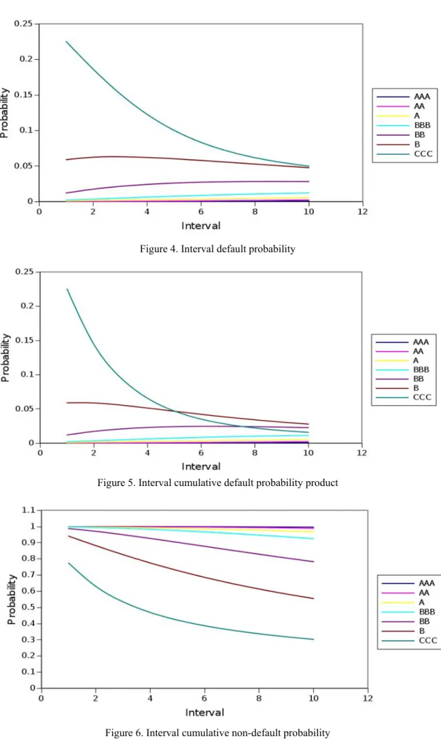
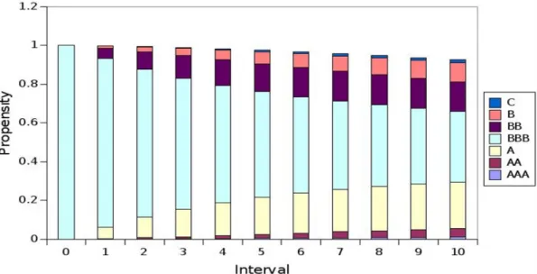
In line with reduced form models, Elton et al (2001) develop marginal default probabilities from a rating transition matrix employing the assumption that the rating transition process is stationary and Markovian. In year one, the marginal probability of default can be determined directly from the transition matrix and default vector, and is, for each rating class, the proportion of defaults in year one. To obtain subsequent year defaults, they first use the transition matrix to calculate the ratings going into a given year for any bond starting with a particular rating in the previous year. The defaults of that year are then the proportion in each rating class multiplied by the probability that a bond in that class defaults by year end. They find that the marginal probability of default increases for the high-rated debt and decreases for the low-rated debt. This occurs because bonds change rating classes over time.
Elton et al (2001) show that a bond rated AAA has zero probability of defaulting one year later. However, given that it has not previously defaulted, the probability of it defaulting 20 years later is 0.206 percent. In the intervening years, some of the bonds originally rated AAA have migrated to lower-rated categories where there is some probability of default. At the other extreme, a bond originally rated CCC has a probability of defaulting equal to 22.052 percent in the next year, but if it survives 19 years the probability of default in the next year is only 2.928 percent. If it survives 19 years, the bond is likely to have a higher rating. Despite this drift, bonds that were rated very highly at time 0 tend to have a higher probability of staying out of default 20 years later than do bonds that initially had a low rating. However, rating migration means this does not hold for all rating classes. For example, after 12 years the conditional probability of default for CCCs is lower than the default probability for Bs. This is because the odds of being upgraded to investment grade conditional on not defaulting is higher for CCC than B. Eventually, bonds that start out as CCC and continue to exist will be rated higher than those that start out as Bs. In short, the small percentage of CCC bonds that continue to exist for many years end up at higher ratings on average than the larger percentage of B bonds that continue to exist for many years.
Grandes and Peter (2005) note that the rating agencies’ main justification for the sovereign ceiling rule - namely, that whenever a government defaults, firms in the country will default as well (i.e., transfer risk is 100 percent) - implies that a 1 percent increase in the government spread should be associated with an increase in the firm spread of at least 1 percent. Market participants may judge transfer risk to be less than 100 percent though. The distinguishing feature of industrial countries - and the United States in particular - is that government bonds are risk-free (i.e., sovereign risk is zero). This is in sharp contrast to emerging markets where - almost by definition - government bonds are not risk-free. In an emerging market, the corporate yield spread above an equivalent government bond yield does not reflect corporate default risk, even after controlling for all other factors. It merely reflects corporate default risk in excess of sovereign default risk. Hence, it appears that in emerging economies there is a crucial additional determinant of corporate default risk: the default risk of the government, i.e., sovereign risk.
When a sovereign is in distress or default, economic and business conditions are likely to be hostile for most firms: the economy will likely be contracting, the currency depreciating, taxes increasing, public services deteriorating, inflation escalating, and interest rates soaring, and bank deposits may be frozen. In particular, the banking sector is more likely than any other industry to be directly or indirectly affected by a sovereign in payment problems. The banks’ vulnerability is due to their high leverage (compared to other corporates), their volatile valuation of assets and liabilities in a crisis, their dependence on depositor confidence, and their typically large direct exposure to the sovereign. As a result, default risk of any firm is likely to be a positive function of sovereign risk. They model corporate default probability as the probability that the firm defaults given that the sovereign does not default, plus the probability that the firm defaults given that the sovereign has defaulted.
Fei et al (2012) note a credit rating is a financial indicator of an obligor’s level of creditworthiness. Given the relationship between credit ratings and default probability or credit quality, Kumar and Haynes (2003) discuss rating methodology and list the key factors considered as: i) business analysis (industry risk; market position; operating efficiency; legal position), ii) financial analysis (accounting quality; earnings protection; adequacy of cash flows; financial flexibility; interest and tax sensitivity), and iii) management evaluation (track record of management; evaluation of capacity to overcome adverse situations; goals, philosophy and strategies). They find that financial parameters reflect, to a significant extent, the subjective and objective factors used by an expert while rating a debt obligation, with hidden relationships between the financial parameters and associated expert rating.
(Hines et al, 1975; Ederington and Goh, 1998; Amato and Furfine, 2004). Amato and Furfine (2004) mention that rating agencies insist that their ratings should be interpreted as ordinal rankings of default risk that are valid at all points in time, rather than absolute measures of default probability that are constant through time. Delianedis and Geske (2003) note that rating agencies regularly measure the historical default frequency of corporate issuers. While these historical default frequencies are interesting, they are not forward-looking. Option models can provide a forward-looking, risk neutral default probability. Chan and Jegadeesh (2004) point to evidence that agency ratings may not be accurate in a timely fashion.
Studies like Wang (2004) attempt to model default ratings, and studies like Hines et al (1975), Kaplan and Urwitz (1979), Belkaoui (1980) and Chan and Jegadeesh (2004) statistically model bond ratings. This may provide alternative default probability estimates, as structural models also do, relative to the credit ratings of credit rating agencies, but must still be translated to default probability term structures, in a similar way credit agencies' ratings are translated. In general, bond valuation models - whether structural or reduced form - either use these models to extract default probability estimates from market data, or substitute externally sourced default probability estimates into these models, to determine the magnitude of the default risk component (Eom et al, 2004; Elton et al, 2001; Huang and Huang, 2012; Geske and Delianedis, 2001; Collin‐Dufresne et al, 2001). Also, a number of studies quantify credit ratings as proxies of credit quality in terms of spread (Foss, 1995; Kaplan and Urwitz, 1979; Cantor et al, 1997; Perraudin and Taylor, 2004; Chan and Jegadeesh, 2004)
1.4 Default Probability Term Structures
Elton (1999) argues that realized returns are a very poor measure of expected returns and that information surprises highly influence a number of factors in an asset pricing model. He believes that developing better measures of expected return and alternative ways of testing asset pricing theories that do not require using realized returns have a much higher payoff than any additional development of statistical tests that continue to rely on realized returns as a proxy for expected returns. He argues that either there are information surprises that are so large or that a sequence of these surprises is correlated so that the cumulative effect is so large that they have a significant permanent effect on the realized mean. Furthermore, these surprises can dominate the estimate of mean returns and be sufficiently large that they are still a dominant influence as the observation interval increases. Thus, the difference between expected and realized returns is viewed as a mixture of two distributions, one with standard properties and the other that more closely resembles a jump process.
Duffie and Singleton (1999) state that, because of the possibility of sudden changes in perceptions of credit quality, particularly among low-quality issues such as Brady bonds, one may wish to allow for surprise jumps in default probability.
Nelson and Siegel (1987) state the range of shapes generally associated with interest rate term structures: monotonic, humped, and S shaped. Related to this, Benkert (2004) consider low interest rates with a recessionary state of the economy. Corporate defaults occur more often during economic downturns than during boom phases, and the occurrence of a recession may cause a decline in credit quality that leads to more defaults in the future. According to this line of reasoning, the compensation for default risk would rise. Duffie and Singleton (1999) note strong evidence that hazard rates for default of corporate bonds vary with the business cycle. Equally, recovery data also exhibit a pronounced cyclical component. Das and Tufano (1995) allowed recovery to vary over time so as to induce a non-zero correlation between credit spreads and the riskless term structure. However, for computational tractability they maintained the assumption of independence of the hazard rate (default rate) and risk-free rate.
Huang and Huang (2012) argue that a credit risk premium is required by investors because the uncertainty of default loss should be systematic - bondholders are more likely to suffer default losses in bad states of the economy. Moreover, precisely because of the tendency for default events to cluster in the worst states of the economy, the credit risk premium can be potentially very large. Athanassakos and Carayannopoulos (2001) note that yield spreads are greater during recessions than during recoveries, and also point to the link between the behaviour of yield spreads to the shape of the term structure, as a proxy of the business cycle. They confirm the typical direct relationship between default risk and yield spreads, and show that the impact of the business cycle (macro-economy) on the yield spread of a corporate bond depends on the industry sector to which the issuer of the bond belongs. The inflation rate should be directly related to yield spreads, since during inflationary periods investors may require higher risk premia from their investments in corporate bonds.
Athanassakos and Carayannopoulos (2001) use the change in the shape of the term structure of interest rates - represented by the quarterly change in the difference between the 20-year treasury rates and the three month t-bill rates - as a proxy for the business cycle, since much research in the past has linked the shape of the treasury term structure to future variations in the business cycle. A steepening term structure is a typical result of robust economic growth and
lower short term interest rates and reflects a general belief in a more robust economic future. The opposite is true when the term structure is flattening or turns negatively sloped. Therefore, the particular proxy should be negatively related to yield spreads. Finally, the annual rate of change in the industrial production index should be negatively related to yield spreads since increased economic activity will bolster investors’ confidence in the corporate sector, and lead to a reduction in the risk premia demanded for investment in corporate bonds.
Amato and Furfine (2004) argue that financial market participants behave as if risk is countercyclical, e.g. at its highest during economic downturns. Empirical models, too, tend to indicate a rise in risk during recessions. There is a relationship between the correlation of default rates and loss in the event of default and the business cycle. Models that assume independence of default probabilities and loss given default will tend to underestimate the probability of severe losses during economic downturns. They delineate the empirical significance of the procyclicality of credit quality changes by showing that estimated credit losses are much higher in a contraction relative to an expansion.
Delianedis and Geske (2003) note the term structure of default probabilities could be interesting for examining the changing credit structure of either individual firms, industries, or the whole economy. Thus, a term structure of default probabilities could contain information about the business cycle. Typically, the term structure of unconditional default probabilities should be upward sloping because the probability of default over a specific time horizon increases with time. However, the term structure of default probabilities would be inverted when the short term default probability is greater than the forward default probability. This may occur whenever the firm has a high probability of defaulting in the short term, but if it can survive through the next year and payoff its short term obligations, then the firm’s default probability might decline. In this situation, the forward default probability would be less than the short term default probability. The short probability relates to the probability of only defaulting on the short term debt, and the forward probability held today relates to the probability of defaulting on the long term debt, conditional on not defaulting on the short term debt.
Longstaff and Schwartz (1995) argue that the corporate yield spread should vary inversely with the benchmark treasury yield, and find evidence to support this. Kim et al (1993) show that default risk is not particularly sensitive to the volatility of interest rates but is sensitive to interest rate expectations. Campbell and Taksler (2003) note idiosyncratic volatility can move very differently from market-wide volatility. Movements in idiosyncratic risk are more persistent than movements in market risk. Lando and Skødeberg (2002) note that it is likely that macroeconomic variables or other indicators of the business cycle influence rating intensities.
Hamilton and Cantor (2004) raise the notion of a credit cycle. This can be studied parallel to business cycles.
A number of studies model default probability term structures as instantaneous stochastic processes (Das and Tufano, 1995; Duffee, 1999; Jarrow et al, 2002) . For example, Duffee (1999) uses the extended Kalman filter to fit yields on bonds issued by individual investment-grade firms to a model of instantaneous default risk. Das and Tufan (1995) and Jarrow et al (1997) model default risk as Markov chains or trees. Jarrow and Turnbull (1995) exogenously specify a stochastic process for the evolution of the default-free term structure and the term structure for risky debt.
Duffee (1999) argues that at each instant there is some probability that a firm defaults on its obligations. Both this probability and the recovery rate in the event of default may vary stochastically through time. The stochastic processes determine the price of credit risk. Although these processes are not formally linked to the firm's asset value, there is presumably some underlying relation. The instantaneous probability that a given firm defaults on its obligated bond payments follows a translated single-factor square-root diffusion process, with a modification that allows the default process to be correlated with the factors driving the default-free term structure. Realistically there are a number of factors other than default risk that drive a wedge between corporate and Treasury bond prices, such as liquidity differences, state taxes, and special repo rates. Here, all of these factors are substituted into a stochastic process called a default risk process. Default risk is negatively correlated with default-free interest rates. In addition, for the typical firm, the instantaneous risk of default has a lower bound that exceeds zero. In other words, even if a firm's financial health dramatically improves, the model implies that yield spreads on the firm's bonds remain positive.
Duffee (1999) first models the price of a risk-free bond as given by the expectation, under the equivalent martingale measure, of the cumulative discount rate between t and T. The discount rate follows a stochastic process - the sum of a constant, and two factors that follow independent square-root stochastic processes. He then models the adjusted discount rate for bond issues that can default, relative to risk-free bonds. This setup is designed to capture three important empirical features of corporate bond yield spreads. The most obvious is that the spreads are stochastic, fluctuating with the financial health of the firm. The second feature is that yield spreads for very high-quality firms are positive, even at the short end of the yield curve. This fact suggests that regardless of how healthy a firm may seem, there is some level below which yield spreads cannot fall. The third feature is that yield spreads, especially spreads for lower quality bonds, appear to be systematically related to variations in the default-free term structure.
Houweling and Vorst (2005) note reduced form models that use time series estimation to model the hazard rate stochastically, typically as a Vasicek or CIR process. Also, other reduced form models use cross-sectional estimation and consider either constant or stochastic hazard rates, where the stochastic process is chosen in such a way that the survival probability curve is known analytically. Houweling and Vorst (2005) follow an intermediate approach by using a deterministic function of time to maturity. This specification facilitates parameter estimation, while still allowing for time-dependency. They model the integrated hazard function as a polynomial function of time to maturity, with three degrees - linear, quadratic and cubic.
Das and Tufano (1995) choose to make recovery rates correlated with the term structure of interest rates. This results in a model wherein credit spreads are correlated with interest rates, as is evidenced in practice. In the Jarrow-Lando-Turnbull model credit spreads change only when credit ratings change, whereas in the debt markets it is found that credit spreads change even when ratings have not changed. Injecting stochastic recovery rates into the model provides this extra feature.
Hamilton and Cantor (2004) point out the strong stochastic processes associated with rating transitions. Altman and Rijken (2004) investigate the through-the-cycle methodology that agencies use. Through the cycle ratings are stable because they are intended to measure the risk of default over long investment horizons, and because they are changed only when agencies are confident that observed changes in a company's risk profile are likely to be permanent. Investors believe that ratings should reflect changes in credit quality, even if they are likely to be reversed within a year. At the same time, investors want to keep their portfolio rebalancing as low as possible and desire some level of rating stability. This leaves two conflicting goals - rating timeliness and rating stability. The objective of agencies is to provide an accurate relative (ordinal) ranking of credit risk at each point in time, without reference to an explicit time horizon. The through-the-cycle rating methodology of agencies is designed to achieve an optimal balance between rating timeliness and rating stability. The methodology has two key aspects: first, a long-term default horizon and, second, a prudent migration policy. These two standpoints are aimed at avoiding excessive rating reversals, while holding the timeliness of agency ratings at an acceptable level. Compared to point-in-time ratings, agency ratings are aimed at ignoring temporary shocks.
In relation to credit rating migration matrices, Altman (1996) assesses the rating change experience of corporate bonds from two different initial states: i) from the time of issuance to up to ten years post-issuance, and ii) from a static-pool of issuers of a given rating, regardless of the bonds' ages, to up to ten years after the pool is formed. In contrasting unexpected and expected rating migration, he notes the standard deviation around the expected value could be calculated.
Frydman and Schuermann (2008) note that, despite overwhelming evidence to the contrary, credit migration matrices, used in many credit risk and pricing applications, are typically assumed to be generated by a simple Markov process. In their paper they propose a parsimonious model that is a mixture of (two) Markov chains. They estimate this model using credit rating histories and show that the mixture model statistically dominates the simple Markov model and that the differences between two models can be economically meaningful. The non-Markov property of their model implies that the future distribution of a firm’s ratings depends not only on its current rating but also on its past rating history. They find that two firms with identical current credit ratings can have substantially different transition probability vectors. Lando and Skødeberg (2002) contrast rating migration matrices captured by means of a discrete-time estimator, and continuous-time estimator. The continuous-time estimator captures the chance of defaulting within a year after successive downgrades, even if it did not happen for one single firm in the sample, whereas the discrete-time method does not. It is shown that rating migration matrices from these different methods differ significantly. They present a rigorous formulation of the notion of rating drift - a type of non-Markovian behavior - in the process of ratings and find strong non-Markov effects for downgrades.
Nickell et al (2000) use Moody’s data from 1970 to 1997 to examine the dependence of ratings transition probabilities on industry, country and stage of the business cycle using an ordered probit approach, and they find that the business cycle dimension is the most important in explaining variation of these transition probabilities. They point out that rating transition matrices vary according to the stage of the business cycle, the industry of the obligor and the length of time that has elapsed since the issuance of the bond. Kadam and Lenk (2008) identified strong differences in rating migration behaviour between issuers of different industry sectors and countries.
Bangia et al (2002) argue that credit migration matrices provide the specific linkage between underlying macroeconomic conditions and asset quality. Credit migration matrices characterize the expected changes in credit quality of obligors. Total volatility (risk) is composed of a systematic and an idiosyncratic component. Because ratings are a reflection of a firm’s asset quality and distance to default, a reasonable definition of “systematic” is the state of the economy. They find distinct differences between the U.S. expansion and contraction transition matrices. The most striking difference between expansion and contraction matrices are the downgrading and especially the default
probabilities that increase significantly in contractions. Overall, these results reveal that migration probabilities are more stable in contractions than they are on average, supporting the existence of two distinct economic regimes. The rating universe should develop differently in contraction periods compared to expansion times.
The straightforward application of these matrices however would normally be restricted to situations where the future state of the economy over the transition horizon under consideration is assumed to be known. The state of the economy clearly is one of the major drivers of systematic credit risk, especially as lower credit classes are much more sensitive to macro-economic factors. Consequently it should be integrated into credit risk modeling whenever possible, otherwise the downward potential of high-yield portfolios in contractions might be severely underestimated. Modern credit risk models account for different industries only through different term structures, but not through industry dependent transition matrices.
Fei et al (2012) proposes an approach to estimate credit rating migration risk that controls for the business-cycle evolution during the relevant time horizon in order to ensure adequate capital buffers both in good and bad times. The approach allows the default risk associated with a given credit rating to change as the economy moves through different points in the business cycle. They mention a body of research linking portfolio credit risk with macroeconomic factors showing, for instance, that default risk tends to increase during economic downturns. Their premise is that point-in-time methodologies that account for business cycles should provide more realistic credit risk measures than through-the-cycle models that smooth out transitory fluctuations (perceived as random noise) in economic fundamentals.
The naïve approach to accommodating cyclicality subdivides the historical ratings into those observed in normal, peak and trough regimes according to real GDP growth and deploys a discrete time (cohort) estimator of migration risk separately on each sub-sample. In effect, the naïve estimator implicitly assumes that the current economic conditions prevail throughout the prediction time horizon of interest. They relax this assumption by allowing the economy to evolve randomly between states of the business cycle during the risk horizon, and evaluate a MMC estimator against a naïve counterpart that conditions deterministically on the current economic conditions by assuming that they prevail throughout the prediction time horizon, and against classical through-the-cycle estimators. Such studies consider economic dynamics in credit risk modelling, by assessing the estimators in a strictly forward-looking sense. In contrast, they exploit a real-time leading indicator of business cycles based on a principal components methodology to generate out-of-sample predictions of credit migration risk. Acknowledging the risk that economic conditions randomly evolve over the risk horizon is shown to improve the accuracy of out-of-sample default probability predictions. Ignoring business cycles significantly understates default risk during economic contraction.
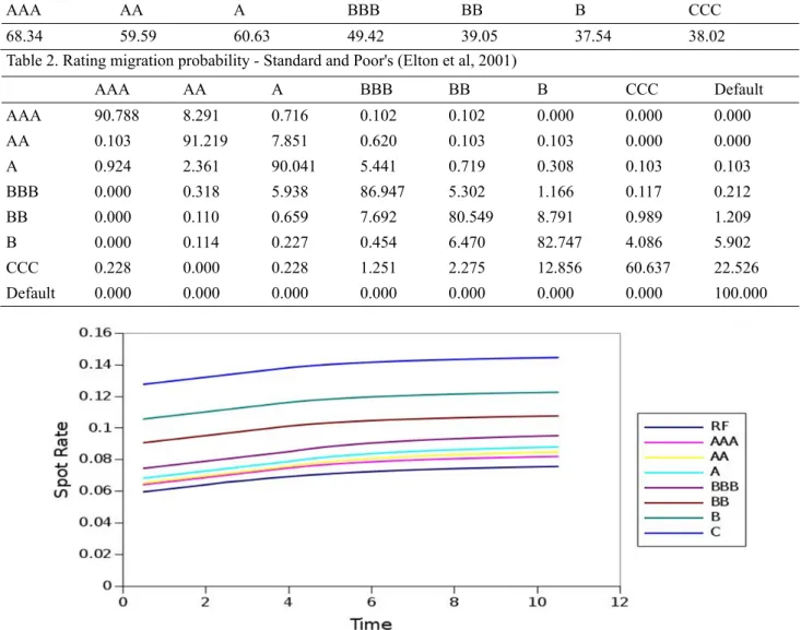
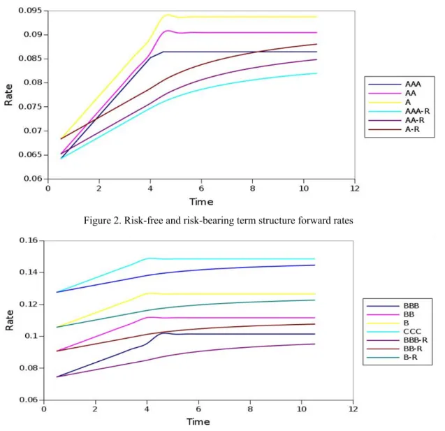
Elton et al (2004) consider factors that affect individual issue prices, as part of homogeneous groups of bonds. They then assume that each of the variables considered could effect the level but not the shape of the corporate term structure. For example, it is assumed that the Baa+ and Baa- spot term structure curves are parallel to each other and the Baa spot term structure curve. They note that, to the extent that this simplification of the effect of variables is inappropriate it will bias their results against attributing importance to the influences they examine. Also, there exists significant correlation between homogeneous corporate term structures, in that such term structures generally lay parallel to each other, and perhaps even the market corporate term structure. A number of studies also allude to some correlation between risk-bearing term structures and default probability term structures (Elton et al, 2001; Eom et al, 2004).
1.5 A Rating Migration Based Valuation Model
1.5.1 A Rating Migration Based Reduced Form Model for Zero-Coupon and Coupon Paying Risk-Bearing Bonds Equation 1 states the reduced form model of Duffie and Singleton (1999), adapted for coupon paying bonds. Equation 1 has two components, a coupon paying component associated with non-default outcomes, and a recovery component associated with default outcomes.
In the equation, 𝑉 is the price or value of the risk-bearing bond; 𝑀 is the number of coupons of the bond, including par; 𝐶 is the coupon of the bond on coupon date 𝑚; 𝑅 is the recovery of par value; 𝑟 and 𝑡 are the risk-free spot rate and time value, respectively, associated with coupon date 𝑚; ℎ is the default probability of interval 𝑛, conditional on no default prior to interval 𝑛; 𝑃 is the cumulative non-default probability of interval 𝑚; 𝐽 is the number of probability intervals for which the possibility of default is considered up to coupon date 𝑚; 𝐽 is the number of probability intervals considered up to maturity.
For coupon paying bonds, it is convenient to consider 𝐽 and 𝐽 to be equal to 𝑚 and 𝑀. For example, the third coupon may have three probability intervals leading up to it. For zero-coupon bonds, 𝑀 is equal to 1, and 𝐽 may be greater than 𝑀, with 𝐽 not necessarily corresponding with m ; a regular coupon interval may still be considered though to ensure a timely and consistent consideration of default. A five-year zero coupon bond will have only one
coupon, but can have up to ten probability intervals leading up to it, if semi-anual probability intervals are used. 𝑉 = 1 − ℎ 𝑒 𝐶 + 1 − ℎ ℎ 𝑒 𝑅 (1.1) 1 − ℎ = 1 ; 𝑗 − 1 1 (1.1.1) 𝑃 = 1 − ℎ (1.2) 𝑃 | = 1 − ℎ − 1 − ℎ = 1 − ℎ 1 − 1 − ℎ = 1 − ℎ ℎ (1.3)
𝑉 =
𝑃 𝑒
𝐶
+
𝑃
|𝑒
𝑅
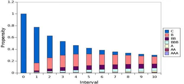
(1.4)Although not explicitly stated by them, equation 2 delineates the default probability structure implemented by Elton et al (2001). They subsequently substitute this into a reduced form model similar to equation 1.
𝑐𝑎𝑡 are all non-default rating categories; 𝐼 ℎ is the intensity or propensity of path or tree Pathm that leads up to interval 𝑚; similarly, 𝐼 ℎ is the path intensity or propensity of path 𝑗; 𝐼
is the intensity or propensity of rating category n in interval m ; 𝑃𝑎𝑡ℎ is the number of default paths of (up to) interval 𝑚;
𝑃𝑎𝑡ℎ is the number of non-default paths of interval 𝑚; contrary to a default path, a non-default path can not and does not end up in default over its length or run; 𝑃𝑎𝑡ℎ | → is the number of non-default paths that migrate to - end with - category 𝑘in interval m ; 𝑃 | → is the probability of migration from rating 𝑏 in interval 𝑛 − 1 to rating 𝑏 in interval n; 𝑃 → | is the probability of migration from category 𝑘 to category 𝑛
in interval m ; 𝑃 → | is the probability of category 𝑘 migrating to default status in interval 𝑚; ℎ is again the default probability of interval 𝑛, conditional on no default prior to interval 𝑛.
𝐼 ℎ = 𝑃 | → (2.1) 𝐼 = 𝐼 ℎ ℎ | → 𝑃 → | = 𝐼 𝑃 → | (2.2)
∏
n=1 m(
1
−
h
n) =
∑
n=1 Pathm non−defaultI
n Path=
∑
n=1catnon−default
I
mcatn (2.3)
1 − ℎ ℎ = 𝐼
| →
ℎ = 1 − 1 − ℎ / 1 − ℎ = 𝐼 𝑃 → | / 1 − ℎ (2.5)
Equation 3 allows the recovery rate to depend on the rating category the bond is in when it defaults. Moving from equation 1.4 to equation 3.1 is further explained by equation set 2. 𝑅 is the recovery of par value of rating category 𝑛
in interval 𝑚.
𝑉 = 𝑃 𝑒 𝐶 + 𝐼 𝑃 → | 𝑒 𝑅 (3.1)
By using a value loss description, equation 1 is rewritten as the sum of all promised cash flows, discounted at the risk-free rate, minus the present value of value lost due to default. It is expected that equation 4 should yield a similar value than equation 1.
𝑉 | is the risk-free based value of a bond with rating category 𝑎, in interval 𝑚; 𝐹𝑉 | is the risk-free based future value of a bond of rating category 𝑎, in interval 𝑚; 𝛥𝑉 → is the change in value due to a bond of rating category 𝑎 defaulting in interval 𝑚; 𝑟 | is the risk-free forward rate over the interval demarcated by point in time
𝑛 and 𝑚; 𝑅 is the recovery of par value of rating category 𝑛 in interval m ; 𝐼 is the intensity or propensity of rating category 𝑛 in interval m ; 𝑃 → | is the probability of category 𝑘 migrating to default status in interval 𝑛; 𝑟 and 𝑡 are the risk-free spot rate and time value, respectively, associated with coupon date 𝑚;
𝑃𝑉 𝑥 refers to the present value of 𝑥; 𝑐𝑎𝑡 are all non-default rating categories; 𝑘 is the number of coupons remaining at (after) interval 𝑚.
𝑉 | = 𝐹𝑉 | = 𝑒 | 𝐶 (4.1)
𝛥𝑉 → = 𝐼 𝑃 → | 𝑉 | − 𝑅 (4.2)
𝑉 = 𝑒 𝐶 − 𝐼 𝑃 → | 𝑃𝑉 𝑉 | − 𝑅 (4.3)
𝑉 = 𝑒 𝐶 𝐼 𝑃 → | 𝑒 𝑅 − 𝑉 | 𝑒 (4.4)
1.5.2 Credit Quality Deterioration, Rating Migration, and Valuation According to Rating Migration
In certain markets, like the South African market, credit spreads persist, yet the market has experienced very low default rates. Not all (few) corporate bonds in this market have top credit ratings assigned to them by credit agencies, and credit spreads abound. At the same time, historically very few actual defaults have occurred, such that a rating migration matrix based on historical data would have extremely low probability of migration to default per credit rating category. In light of credit risk being synonymous with credit quality, equation 5 rather values a bond according to its likely future credit ratings and thus credit quality. Bonds may very well migrate to a lower rating and thus credit quality, and remain there for some time, without defaulting immediately, or defaulting at all - the bond has merely migrated to a higher probability of default, and a rating homogeneous portfolio the bond forms part of, is expected to honour this probability of default estimate.
probability of default in the future. For a risk-neutral investor to be indifferent to the investment period, future credit quality must be adequately anticipated. Credit quality changes in the form of rating migration may cause an investor to reconsider holding a security, particularly in light of expected future ratings and thus credit quality, if it was not properly included in the valuation beforehand. This implies that the investor is not insensitive - but indeed sensitive - to the investment period.
Thus, a bond may also be valued according to its probable future rating states, which corresponds to the rating migration paths of equation 2. In addition, this should produce a result comparable to a valuation that considers expected cash flows, when considering the risk of default (equation 1, 3 and 4). The duration of a bond in a particular rating category is valued against the forward rate of that category for the given duration or interval. The value of a bond is thus seen as the sum of the present value of all possible future rating states, according to all possible rating migration paths (equation 5.2). For this purpose, a rating migration matrix is still used. Practically, the study uses the market risk-bearing term structures to value these future rating states.
As equation 5.4 and 5.5 reflect, the forward rate applicable over a particular rating migration path is seen as an extra weight or attenuation factor, such that that the intensity or propensity of a particular sub-path - and thus path - is simply the probability of the path multiplied by the applicable forward rate.
Much of the terms correspond to that of previous equations. 𝑀 is the number of coupons of the bond, including par value; Cm is the bond coupon corresponding to coupon date 𝑚; 𝑅 is the recovery of par value; 𝑅 is the recovery of par value of rating category 𝑛 in interval 𝑚; 𝑐𝑎𝑡 are all non-default rating categories;
𝑃𝑎𝑡ℎ | → is the number of non-default paths that migrate to - end with - category 𝑘in interval 𝑚; 𝑃𝑎𝑡ℎ is the number of default paths of interval 𝑚; 𝑃𝑎𝑡ℎ is the number of non-default paths of interval 𝑚;
𝑃 ℎ is the probability of path 𝑛 over interval 𝑘; 𝑡 is the time interval length between interval 𝑘 and 𝑘 − 1;
𝐷𝐹 | is the discount factor of rating category 𝑎 over the interval demarcated by point in time 𝑚 and 𝑛 - this also corresponds with the forward rate of the rating category over the interval; 𝐷𝐹 | ℎ is the discount factor of path 𝑛
over the interval (𝑘 − 1, 𝑘), which equals the forward over the particular interval; 𝑓 | is the forward rate of rating category 𝑛 over the interval 𝑚 and 𝑚 − 1; 𝑓 ℎ | is the forward rate of path nover interval 𝑘; IPathl
df
and 𝐼 | ℎ are the forward rate based path intensity or propensity of path l; 𝐼 | is the forward rate based intensity or propensity of rating category 𝑛 in interval 𝑚; 𝑃 → | is the probability of migration from category 𝑘 to category 𝑛 in interval 𝑚; 𝐽 is the number of probability intervals considered up to coupon date 𝑚.
𝐷𝐹 | = 𝐷𝐹 | / 𝐷𝐹 | = 𝑒 (5.1) 𝑉 = ℎ 𝑃 ℎ 𝐷𝐹 | ℎ 𝐶 (5.2) 𝑉 = ℎ 𝑃 ℎ 𝑒 ℎ | 𝐶 (5.3) 𝐼 ℎ = 𝑃 | → 𝑒 ℎ | (5.4)
𝐼 | = ⎝ ⎛ 𝐼 | ℎ ℎ | → 𝑃 → | 𝑒 | ⎠ ⎞ = 𝐼 | 𝑃 → | 𝑒 | (5.5) 𝑉 = 𝐼 | 𝐶 (5.6)
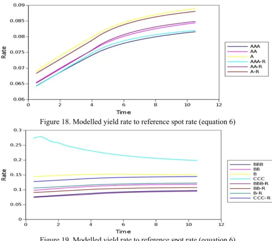
Equation 6 includes the cash flows gained from recovery of par, after default. The recovery cash flow component is taken from equation 1. Again, 𝑟 and 𝑡 are the risk-free spot rate and time value, respectively, associated with coupon date 𝑚; 𝑃 → | is the probability of category 𝑘 migrating to default status in interval 𝑛.
𝑉 = 𝑃 ℎ 𝑒 ℎ | 𝐶 ℎ + 𝑃 ℎ ℎ 𝑒 𝑅 (6.1) 𝑉 = 𝐼 | 𝐶 + 1 − ℎ ℎ 𝑒 𝑅 (6.2) 𝑉 = 𝐼 | 𝐶 + 𝐼 𝑃 → | 𝑒 𝑅 (6.3)
Equation 7 calculates the net change in value at point m due to rating migration over the remaining probability intervals from that point to maturity. It is calculated as the sum of the change in future value for each remaining probability interval, up to maturity, based on rating migration per interval.
𝐷𝐹 | is the discount factor of rating category 𝑎 over the interval demarcated by point in time 𝑛 and m; 𝑟 | is the forward rate of rating category 𝑎 over the interval demarcated by point in time 𝑛 and 𝑚; 𝑟 is the spot rate of rating category 𝑎 over the interval n ; 𝑟 is the risk-free spot rate associated with point in time 𝑚; 𝑡 is the interval demarcated by point in time n and 𝑚; 𝐹𝑉 is the future value of a bond of rating category 𝑎, in interval 𝑚; 𝑉 is the value of a bond with bond rating 𝑎, in interval 𝑚; 𝛥𝑉 → is the change in value of a bond due to a rating migration from rating 𝑎 to 𝑏 in interval 𝑚; 𝛥𝑉 is the change in value of a bond with rating category 𝑎 due to rating migration to any other non-default rating category in interval 𝑚; 𝐼 is the intensity or propensity of rating category 𝑛 in interval 𝑚; 𝑃 → | is the probability of migration from category 𝑘 to category 𝑛 in interval 𝑚;
𝑀is the number of coupons of the bond, including par value; 𝐶 is the bond coupon corresponding to coupon date 𝑚;
𝑐𝑎𝑡 are all non-default rating categories; 𝑃𝑉 𝑥 refers to the present value of 𝑥; 𝑅 is the recovery of par value of rating category 𝑛 in interval 𝑚; 𝑘 is the number of coupons remaining at (after) interval 𝑚.
𝐷𝐹 | = 𝐷𝐹 | / 𝐷𝐹 | = 𝑒 ; 𝑟 | 𝑡 = 𝑟 𝑡 − 𝑟 𝑡 (7.1)
𝛥𝑉 → = 𝐹𝑉 − 𝐹𝑉 = 𝑉 − 𝑉 (7.3) 𝛥𝑉 → = 𝑒 | 𝐶 − 𝑒 | 𝐶 = 𝑒 | − 𝑒 | 𝐶 (7.4) 𝛥𝑉 = 𝐼 𝑃 → | 𝛥𝑉 → = 𝐼 𝑃 → | 𝑒 | − 𝑒 | 𝐶 (7.5) 𝛥𝑉 = 𝑃𝑉 𝛥𝑉 = 𝛥𝑉 𝑒 (7.6)
Equation 8 states the value of a bond as the present value of coupons received up to future point 𝑤, plus the present value of the future value of the bond at point 𝑤; point 𝑤 is before maturity. In essence, it states the value of the bond when the bond is not kept to maturity, but sold before maturity. Equation 8.2 states the future value of the bond according to the present value of coupons to be received after point 𝑤 (equation 3). Equation 8.3 states the future value according to the present value of the future paths of the bond after point 𝑤 (equation 6). Equation 8.4 states the future value as the sum of the value of the remaining bond coupons at time 𝑤, discounted against the rating categories’ future rates at point 𝑤, and weighed according to the rating categories’ propensities at point 𝑤 - for each rating category, its propensity is considered at point 𝑤, and all remaining coupons are discounted against the future rates of the rating category at point 𝑤. Again, some similarity and convergence is expected among the equations - the equations should produce similar results. For equation 8.3 to equal equation 6, the future value of the bond is not discounted to present value by the risk-free rate, but by the rating path based spot rate 𝑅 .
𝐶 is the coupon of the bond on coupon date 𝑚; 𝑘 is the number of coupons up to point 𝑤; 𝑅 is the recovery of par value of rating category 𝑛 in interval 𝑚; 𝑃 is the cumulative non-default probability of interval 𝑚; 𝑟 and
𝑡 are the risk-free spot rate and time value, respectively, associated with coupon date 𝑚; 𝑟 is the risk-free forward rate over the interval (𝑤, 𝑚) - 𝑡 ; 𝑟 is the risk-bearing forward rate of rating category 𝑛 over the interval (𝑤, 𝑚);
𝐼 is the intensity or propensity of rating category n in interval 𝑚; 𝐼 | is the forward rate based intensity or
propensity of rating category 𝑛 in interval 𝑚; 𝐼 | is the intensity or propensity of rating category 𝑛 in interval 𝑚, measured from point 𝑤; 𝐼 | | is the forward rate based intensity or propensity of rating category 𝑛 in interval 𝑚, measured from point 𝑤; 𝑃 → | is the probability of migration from category 𝑘 to default in interval 𝑚; 𝑃𝑉 𝑥
refers to the present value of 𝑥; 𝐹𝑉 refers to the future value of the bond at point 𝑤; 𝐽 is the number of probability intervals considered up to coupon date 𝑚; 𝑅 is the risk-bearing rating path based spot rate of rating category 𝑛 for point 𝑤.
𝑃𝑉 𝐹𝑉 = 𝑒 𝑃 𝑒 𝐶 + 𝐼 𝑃 → | 𝑒 𝑅 (8.2) 𝑃𝑉 𝐹𝑉 = 𝐼 | | 𝑒 𝐶 + 𝐼 𝑃 → | 𝑒 𝑅 𝑒 (8.3) 𝐼 | = 𝐼 𝑒 (8.3.1) 𝑃𝑉 𝐹𝑉 = 𝑒 𝐼 𝑒 𝐶 (8.4)
1.5.3 Term Structure Volatility and Term Structure Volatility Premiums
At some point, one or more of the equations above reference the recovery of par, the risk-free rate, risk-bearing rates, and a rating migration matrix as input. The recovery of par, the risk-free rate as term structure, the risk-bearing rate as term structure, and the rating migration matrix can all carry additional volatility as uncertainty. All but uncertainty pertaining to recovery of par is discussed next.
Term structure stability (Marciniak, 2006) is a well-known factor with regards to term structure decomposition, and term structure volatility - variance over term structures pertaining to similar points in time, decomposed at different dates - is also documented (Marciniak, 2006). If the ahistorical risk-free and risk-bearing term structures are accepted as volatile, it should not be difficult to also consider ahistorical rating migration as volatile - that the probability of rating migration to both non-default credit ratings as well as default, is ahistorically uncertain.
Two views can be taken regarding term structure volatility: i) premiums for term structure volatility are already included in term structure spot rates, such that cash flows that reference these rates are already guarded against term structure volatility; ii) premiums for term structure volatility should be added as additional factors of a bond valuation model. Below, options are used to demonstrate the cost of term structure volatility, and options manage to do this quite intuitively. At the same time, the magnitude (cost) of the options may be negligible, suggesting that premiums for term structure volatility are already included in spot rates.
A basic premise of the view that term structure volatility premiums are already included, is that continuously or repetitively rolling over short term investments - investing and re-investing when the investment term expires - in risk-free and risk-bearing bonds should not yield higher returns than a single, long-term investment in the same security type, for the same investment term. As illustration, consider reinvesting in the next bond with 1 year to maturity, when the previous investment expires, and doing so for a period of 5 years, versus investing in a bond with 5 years to maturity. Here, continuously investing and reinvesting in bonds with short time to maturities has the advantage that long term term structure uncertainty is avoided, and market rates at the applicable points in time are likely more reflective of term structure rates at that point. The long-term bond must yield a return at least the same as the repetitive short-term investment, merely to be appropriate in terms of compensation in light of economic conditions. Yet, because it entails more uncertainty, the long-term investment is expected to yield a higher return - only under ideal market efficiency would it yield a similar return than the short term investment.
This highlights the dichotomy between historical and ahistorical, and points out that historical estimates may find it difficult to fully account for and explain ahistorical prices. As long as the long-term investment yields an appropriately higher return than the short-term investment, term structure volatility premiums are likely already included in term structure spot rates. In the above, appropriately higher implies what is humanly possible under practical levels of market efficiency.
In the case that term structure volatility premiums are already included in spot rates, bond valuation models may only be able to examine and state the magnitude of such premiums via i) ahistorical estimates of term structure volatility - or historical estimates as approximation thereof - or ii) isolating the term structure volatility component from the spread