biblio.ugent.be
The UGent Institutional Repository is the electronic archiving and dissemination platform for all UGent research publications. Ghent University has implemented a mandate stipulating that all academic publications of UGent researchers should be deposited and archived in this repository. Except for items where current copyright restrictions apply, these papers are available in Open Access.
This item is the archived peer-reviewed author-version of:
Unsupervised spectral sub-feature learning for hyperspectral image classification
Viktor Slavkovikj, Steven Verstockt, Wesley De Neve, Sofie Van Hoecke, and Rik Van de Walle In: International Journal of Remote Sensing, 37 (2), 309–326, 2016.
http://www.tandfonline.com/doi/abs/10.1080/01431161.2015.1125554
To refer to or to cite this work, please use the citation to the published version:
Slavkovikj, V., Verstockt, S., Neve, W. D., Hoecke, S. V., and Walle, R. V. d. (2016). Unsupervised spectral sub-feature learning for hyperspectral image classification. International Journal of Remote Sensing 37(2) 309–326. 10.1080/01431161.2015.1125554
Full Terms & Conditions of access and use can be found at
http://www.tandfonline.com/action/journalInformation?journalCode=tres20
Download by: [Ghent University], [Viktor Slavkovikj] Date: 12 January 2016, At: 08:24
International Journal of Remote Sensing
ISSN: 0143-1161 (Print) 1366-5901 (Online) Journal homepage: http://www.tandfonline.com/loi/tres20
Unsupervised spectral sub-feature learning for
hyperspectral image classification
Viktor Slavkovikj, Steven Verstockt, Wesley De Neve, Sofie Van Hoecke & Rik
Van de Walle
To cite this article: Viktor Slavkovikj, Steven Verstockt, Wesley De Neve, Sofie Van Hoecke & Rik Van de Walle (2016) Unsupervised spectral sub-feature learning for hyperspectral image classification, International Journal of Remote Sensing, 37:2, 309-326
To link to this article: http://dx.doi.org/10.1080/01431161.2015.1125554
Published online: 12 Jan 2016.
Submit your article to this journal
View related articles
Unsupervised spectral sub-feature learning for hyperspectral
image classi
fi
cation
Viktor Slavkovikja, Steven Verstockta, Wesley De Nevea,b, Sofie Van Hoeckea
and Rik Van de Wallea
aMultimedia Lab, Department of Electronics and Information Systems, Ghent University-iMinds,
Ledeberg-Ghent, Belgium;bImage and Video Systems Lab, Korea Advanced Institute of Science and Technology
(KAIST), Yuseong-gu, Daejeon, Republic of Korea
ABSTRACT
Spectral pixel classification is one of the principal techniques used in hyperspectral image (HSI) analysis. In this article, we propose an unsupervised feature learning method for classification of hyper-spectral images. The proposed method learns a dictionary of sub-feature basis representations from the spectral domain, which allows effective use of the correlated spectral data. The learned dictionary is then used in encoding convolutional samples from the hyperspectral input pixels to an expanded but sparse feature space. Expanded hyperspectral feature representations enable lin-ear separation between object classes present in an image. To evaluate the proposed method, we performed experiments on several commonly used HSI data sets acquired at different loca-tions and by different sensors. Our experimental results show that the proposed method outperforms other pixel-wise classification methods that make use of unsupervised feature extraction approaches. Additionally, even though our approach does not use any prior knowledge, or labelled training data to learn fea-tures, it yields either advantageous, or comparable, results in terms of classification accuracy with respect to recent semi-super-vised methods.
ARTICLE HISTORY
Received 18 June 2015 Accepted 27 October 2015
1. Introduction
Advances in imaging technology have led to the development of imaging spectro-scopy sensors capable of acquiring hyperspectral imagery at high spatial resolution, thus enabling different geological, agricultural, environmental, and land-survey applications. Unlike regular three-band red, green, and blue (RGB) pictures, hyper-spectral images consist of hundreds of hyper-spectral bands covering a wide interval (e.g. solar reflective wavelengths 400–2400 nm) of the electromagnetic spectrum. Due to their vast data quantities and high spectral resolution (at around 10 nm), hyper-spectral images offer great potential for object recognition and classification. Learning algorithms, however, are affected by the Hughes phenomenon (Hughes1968)
CONTACTViktor Slavkovikj [email protected]
VOL. 37, NO. 2, 309–326
http://dx.doi.org/10.1080/01431161.2015.1125554
© 2015 Taylor & Francis
(i.e. the generalization of the learning algorithm is poor since the number of training samples needed tofill the high-dimensional spectral data space is limited).
There are two main ways to create labelled training data of hyperspectral images. The first is throughfield surveys, which provide accurate data but are expensive and time consuming. The second involves manual labelling of samples through visual recognition. In this method, experts provide the ground truth with the aid of digital elevation maps. However, the spatial resolution of these images has to be high to be able to discern the different classes represented in a HSI.
Because the collection of ground truth data is still largely a manual task, training samples remain scarce. This renders classification of hyperspectral data problematic, which makes full utilization of the information present in hyperspectral images a challen-ging task. On the other hand, unlabelled hyperspectral data are plentiful and can be used in unsupervised learning algorithms for HSI analysis. Therefore, in this article we propose a hyperspectral classification method based on unsupervised learning of spectral sub-fea-tures. Supervised methods (Sun et al.2014; Charles, Olshausen, and Rozell2011; Castrodad et al.2011) using learned dictionaries of spectral pixels have been proposed for hyper-spectral data classification in the past. However, unlike the related supervised methods, our unsupervised approach learns feature representations from subsets of spectral data, which we refer to as spectral sub-feature learning. We evaluate our method based on pixel-wise HSI classification, and show experimental results for commonly utilized hyperspectral remote-sensing scenes (acquired on multiple sites and by different imaging spectroscopy sensors) to compare the effectiveness of this method to state-of-the-art unsupervised and semi-supervised hyperspectral classification techniques.
2. Related work
A number of approaches in HSI classification focus on feature extraction or feature selection as a way to mitigate the problem of dimensionality inherent in hyperspectral data. The main goal of these dimensionality reduction methods is compression or projection of the data into a lower-dimensional subspace such that the intrinsic characteristics of the mani-fold embedded in the high-dimensional hyperspectral data space can be easily discovered. Various feature extraction methods for the purpose of HSI classification have been pro-posed in the literature, including unsupervised methods (Hotelling1933; Chang et al.1999; Wang and Chang2006; Kaewpijit, Le-Moigne, and El-Ghazawi2003; Tenenbaum, de Silva, and Langford2000; Roweis and Saul2000; Belkin and Niyogi2001; Zhang and Zha2005; He et al. 2005; He and Niyogi 2004; Zhang et al. 2007; Qiao, Chen, and Tan 2010), semi-supervised (Cai, He, and Han2007; Chen and Zhang2011; Sugiyama et al.2010; Liao et al. 2013; Shao and Zhang2014), and supervised methods (Bandos, Bruzzone, and Camps-Valls. 2009; Li and Qian2011; Kuo and Landgrebe2004; Kuo et al.2014; Yang et al.2014; Zhong, Lin, and Zhang2014; Tuia et al.2014; Tao et al.2013; Li et al.2011; Sugiyama2007; Chen et al.2014; Chen, Zhao, and Jia2015; Sun et al.2014; Castrodad et al.2011).
2.1. Unsupervised methods
Some well-known unsupervised feature extraction methods used for hyperspectral images are based on principal component analysis (PCA) (Hotelling1933; Chang et al.
1999), independent component analysis (ICA) (Wang and Chang 2006), or discrete wavelet transform (DWT) (Kaewpijit, Le-Moigne, and El-Ghazawi2003). PCA-based meth-ods project the hyperspectral data points onto a lower-dimensional orthogonal sub-space that best preserves their variance, as measured in the high-dimensional hyperspectral data space. On the other hand, ICA-based methods transform the data to independent components by maximizing the non-Gaussianity of the components. In contrast to thefirst two techniques, wavelet transforms decompose hyperspectral data into high- and low-frequency features usingfixed bases.
Although the above methods provide effective data reduction, the global transfor-mations they produce are often insufficiently flexible to represent the local informa-tion content present in hyperspectral images. For example, PCA is unable to discover nonlinear degrees of freedom in the hyperspectral data space, and ICA is less effective when the number of different classes present in an image is large (Wang and Chang2006).
In recent years, unsupervised learning methods for dimensionality reduction, such as isomap (Tenenbaum, De Silva, and Langford2000), locally linear embedding (LLE) (Roweis and Saul2000), Laplacian eigenmaps (LE) (Belkin and Niyogi2001), and local tangent space alignment (LTSA) (Zhang and Zha 2005) have been proposed in the literature. These methods can estimate the intrinsic geometry of a nonlinear mani-fold embedded in a high-dimensional input data space by preserving the local geodesic structure of the data points in the reduced-dimension space. Such local-ity-preserving embedding methods exploit a fundamental property of manifolds, namely, that sufficiently small manifold regions are locally linear. This allows any point to be reconstructed as either a linear approximation (through a linear combi-nation (Roweis and Saul2000; Belkin and Niyogi2001) or local tangent space (Zhang and Zha 2005)) of its neighbours. The reconstruction is invariant to neighbourhood-preserving transformations and is assumed to be the same in dimensionally reduced space. In this way, once the reconstruction weights (Roweis and Saul 2000; Belkin and Niyogi 2001), or local tangent coordinates (Zhang and Zha 2005), are calculated in the high-dimensional space, these can be used to calculate the coordinates of data points by minimizing the reconstruction cost in the reduced dimension space. Similar dimensionality reduction methods, such as neighbourhood-preserving embedding (NPE) (He et al. 2005), locality-preserving projection (LPP) (He and Niyogi 2004), and linear local tangent space alignment (LLTSA) (Zhang et al. 2007), which are linear approximations to LLE, LE, and LTSA, respectively, have been used for feature extraction in hyperspectral images (Huang and Kuo 2010; Liao et al. 2013).
In comparison to the unsupervised feature extraction methods described earlier, our proposed method does not reduce the dimensionality of the HSI data. In con-trast, we learn discriminative features by mapping in an expanded but sparse feature space, which allows for linear separability of the classes present in the hyperspectral image.
In cases when class labels are available, better HSI classification results are reported in the literature from the use of semi-supervised and supervised methods. Therefore, we also briefly review some of the state-of-the-art supervised and semi-supervised learning approaches.
2.2. Supervised methods
Supervised learning methods make use of a priori information about the classes present in the training set. Some supervised feature extraction techniques (Bandos, Bruzzone, and Camps-Valls. 2009; Li and Qian 2011) for hyperspectral images are based on the well-known linear discriminant analysis (LDA) method, which uses labelled samples to find a projection matrix that maximizes between-class variance to within-class variance. Another discriminant-based supervised hyperspectral feature extraction method, called non-parametric weighted feature extraction (NWFE) (Kuo and Landgrebe2004), uses an improved discrimination criterion by assigning a higher weight to samples closer to the discrimination boundary region. Kuo et al. (2014) proposed a kernel-based hyperspectral feature selection method, which optimizes the linear combination ofz-score values of features in the radial basis function kernel. In the work of Yang et al. (2014), an approach inspired by compressive sensing is given which is based on a single-layer feed-forward neural network with sparsity constraints on the input and hidden layer. Deep learning neural network models (Chen et al. 2014; Chen, Zhao, and Jia 2015), based on deep belief networks (DBNs) (Hinton, Osindero, and Teh 2006) and autoencoders (AEs) (Hinton and Salakhutdinov 2006), have also been proposed. These models learn hierarchical features from hyperspectral input data by greedy layer-wise training of restricted Boltzmann machines (RBMs), or layers of hidden units, followed by supervised training of the whole stacked model for the classification task.
A sparse modelling dictionary-based approach has been applied in previous HSI classification methods (Sun et al. 2014; Castrodad et al. 2011; Chen, Nasrabadi, and Tran 2011), where different types of sparsity constraints have been included in the corresponding dictionary modelling cost functions. The general idea behind these methods is to learn a separate dictionary for each class from labelled data (Sun et al. 2014; Castrodad et al.2011), or use the labelled data per se to form dictionaries (Chen, Nasrabadi, and Tran 2011), and classify unknown pixels by determining which class-specific dictionary best describes the sample in terms of minimum value of the recon-struction error. The aforementioned methods use labelled training samples (or at least assume that the classes present in the data set are known a priori (Castrodad et al. 2011)) to obtain class-specific dictionaries, whereas our method uses only unlabelled samples and no prior information to learn a single general dictionary. Furthermore, in the proposed method, features are learned from subsets of data in the spectral domain, whereas the granularity of the dictionary atoms in the related methods is at the pixel level.
Supervised algorithms have recently been developed to take into account both spectral and spatial information in order to improve the classification of multispectral and hyperspectral images (Sun et al.2014; Castrodad et al.2011; Chen, Nasrabadi, and Tran2011; Zhong, Lin, and Zhang2014; Ji et al.2014; Tuia et al.2014; Tao et al.2013; Li et al.2011; Chen et al.2014; Chen, Zhao, and Jia2015). Spatial information can also be used to complement our proposed method. One way of doing this would be to make use of segmentation maps of the scene, or to include the morphological profiles of hyperspectral images (Benediktsson, Palmason, and Sveinsson2005). Another approach relies on methods for combining multiple types of feature (Zhang et al. 2012, 2015; Li
et al.2015). In this study, however, we focus on learning discriminative features from the spectral domain only.
2.3. Semi-supervised methods
Compared with unsupervised and supervised learning approaches, semi-supervised methods for HSI classification make use of only limited labelled data together with unlabelled data. Due to the high costs of creating labelled data sets, as well as the efficacy which can be on a par with that of supervised techniques, semi-supervised learning methods are a viable option for real-world HSI classification applications. Representative semi-supervised methods applied to the classification of hyperspectral images include semi-supervised discriminant analysis (SDA) (Cai, He, and Han2007). SDA uses a graph Laplacian-based regularization constraint in LDA to include local manifold information from unlabelled samples and prevent over-fitting when there are insuffi -cient labelled data. Sugiyama et al. (2010) proposed semi-supervised local Fisher dis-criminant analysis (SELF), which uses a trade-off parameter on the scatter matrices to linearly combine contributions of a supervised method (local Fisher discriminant analysis Sugiyama (2007)) and an unsupervised method (PCA). Liao et al. (2013) introduced semi-supervised local discriminant analysis (SELD). In the same manner as SELF, SELD com-bines supervised LDA with an unsupervised learning method in the category of local linear feature extraction methods (NPE, LPP, or LLTSA). However, unlike SELF, the combination of the contribution of the supervised and unsupervised learning method is nonlinear and non-parametric. Shao and Zhang (2014) use the regularized scatter matrices from SELF with an objective function to combine the advantages of SELF with an unsupervised dimensionality reduction method: sparsity-preserving projection (SPP) (Qiao, Chen, and Tan2010). The contribution of each learning method is then controlled by a trade-offparameter.
3. Spectral sub-feature learning
Recently, significant research efforts in machine learning have been focused on algo-rithms for unsupervised learning of features directly from input data for high-level tasks such as classification and recognition. Much progress has been made in different computer vision tasks (Hinton, Osindero, and Teh2006; Lee et al.2009; Coates and Ng 2011; Coates, Ng, and Lee2011; Yang et al.2009; Wang et al.2010) with models trained on data sets consisting of greyscale or colour images. Inspired by the good performance of these feature learning systems, we propose a method for learning discriminative spectral sub-features from hyperspectral images. Unsupervised feature learning methods for visual object classification typically rely on large sets of (single-channel or RGB) images for training; however, hyperspectral data sets normally consist of a single acquisition of a scene with a large number of channels. Therefore, the proposed algorithm operates directly in the spectral domain, scaling to a large number of spectral bands. Furthermore, by effectively incorporating the information from all available bands, the problem of selection of optimal bands is eliminated.
We build a single-layer model for feature learning. In the first stage, we learn a dictionary of basis vectors using an unsupervised learning algorithm. Two different
algorithms– sparse modelling and a fast stochastic gradient descent (SGD) variant of k-means clustering–were used for learning the basis vectors. In the second stage, the learned basis vectors are applied to map convolutional samples from the spectral pixel space to the feature space with the help of an encoding function (see Figure. 1). Encoded samples are further pooled, which reduces the dimension of thefinal feature vector. We train a linear classifier using the newly obtained feature vectors in order to be able to predict the class of each hyperspectral pixel. In this section, we will describe our proposed approach in more detail.
3.1. Sampling and preprocessing
For training, wefirst sample adjacent hyperspectral bands uniformly at random with a window of width w from unlabelled hyperspectral pixels. As a result, each sample represents a vector in Rw. In this way, we construct a data set X¼xð Þ1;. . .;xð Þn
used for learning basis vectors. Note that throughout this paper we will use Rp and Figure 1.Diagram of feature extraction for HSI classification. Convolutional samples are first extracted from an input pixel. The extracted and preprocessed samples (black circles) are then mapped to feature vectors (blue squares) using the learned mapping functiong:Rw!Rk, wherew denotes the width of the convolutional sampling window andkis the dimensionality of the mapped feature vectors (blue squares). The mapped feature vectors are then locally pooled in blocks. Pooled feature vectors from each block (magenta triangles) are concatenated to obtain the final feature vector.
Rpq to denote a set of p dimensional real-number vectors and a set of pq dimensional real-number matrices, respectively. Each of the vectors xð Þj 2X, j¼ 1;. . .;nis locally normalized to zero mean and unit variance, and the entire data set X is whitened (Hyvärinen and Oja2000) to decorrelate the data. The preprocessed data set X is then used as input to the unsupervised bases learning algorithm. During testing, we extract convolutional samples from each input pixel. That is, we sample windows of widthwof adjacent hyperspectral bands with a stridesbetween windows, as depicted inFigure 1. InSections 3.2and3.3we describe in detail the unsupervised algorithms for learning dictionaries of basis vectors, and the process of feature mapping of convolu-tional samples to obtain thefinal feature vectors.
3.2. Unsupervised learning
The goal of the unsupervised learning algorithm is to learn a dictionary of basis vectors such that a feature mapping functiong:Rw!Rk can be found, which maps an input vector x to a new feature vector y¼gð Þx . We compare two different unsupervised learning algorithms for learning an over-complete dictionary: one based on a sparse modelling approach and the other on an efficient SGDk-means algorithm.
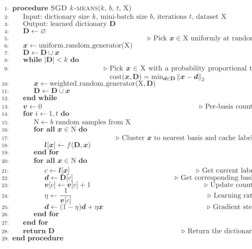
3.2.1. Mini-batch SGDk-means dictionary learning
For the purpose of learning basis vectors from hyperspectral data, we implemented on the graphics processing unit a modified version of an efficient SGD k-means variant (Sculley2010). Because the convergence ofk-means clustering is guaranteed only for a local optimum of its cost function, the clustering result is sensitive to the manner of initialization. Therefore, we employ the initialization procedure proposed by Arthur and Vassilvitskii (2007). The goal of the initialization algorithm is to select each of the initial basis vectors from a different cluster. In order to do so, the initial basis vectors are chosen one at a time, at random, from the data set with probability proportional to the minimum distance of the basis vectors previously chosen. The modified dictionary learning algorithm is given inFigure 2.
3.2.2. Dictionary learning by sparse modelling
The fundamental idea of sparse modelling is learning a dictionary of basis vectors, so that novel input data can be represented as a sparse linear combination of the dic-tionary elements. IfD2Rwk is a dictionary withkbasis elements as columns,A2Rkn represents the sparse decomposition coefficients and X¼xð Þ1;. . .;xð Þn2Rwn is a training data set, then sparse modelling can be represented as a joint optimization problem with respect toDandA:
min D;α 1 n Xn i¼1 1 2kxiDαik 2 2þλ αk ki 1 s:t: "dj2D;j¼1;. . .;k; dTjdj 1: (1)
In (1) an l1 penalty is introduced on the decomposition coefficients αi2A, i¼ 1;. . .;nto yield sparse solutions, whereλis a regularization parameter. The optimization
problem is convex when eitherDorAarefixed, and thus it can be iteratively solved by alternatingly optimizing with respect to one variable (the bases D or coefficients A) while keeping the otherfixed (Lee et al. 2006). Because second-order derivative batch optimization methods can be impractical on large data sets, we use an online dictionary learning algorithm based on stochastic approximations proposed by Mairal et al. (2009).
3.3. Feature mapping, pooling, and classification
Using one of the two previously described unsupervised learning algorithms on an unlabelled training set yields a dictionary of basis vectors that can be used to map novel input samples to feature space. In the case of sparse modelling, the feature space is formed by the obtained sparse decomposition coefficients for the set of input data directly after pooling, which is described below. In the case of the SGDk-means algorithm, we employ the sparse nonlinear encoding transform given by Coates and Ng (2011), which performs a soft assignment of each of themfeatures of the feature vectory¼gð Þx :
Figure 2.K-means algorithm with mini-batch stochastic gradient descent cost minimization.
gmð Þ ¼x max 0ð ;meanð Þ z zmÞ; (2) wherezm¼xdð Þm
2 andd (m)
is them-th basis vector in the learned dictionaryD. In both cases, the feature mapping function transforms an input sample x2Rw to a new sample in feature spacey¼gð Þ 2x Rk.
To obtain the final feature vector for a given hyperspectral input pixel, we first convolutionally sample the pixel’s hyperspectral bands with a window of widthwat a step-sizes(seeFig. 1), and preprocess the extracted samples by employing the same pre processing transforms described inSection 3.1. The extracted samples are then mapped using the learned feature mapping. Finally, the mapped feature vectors are pooled. We perform pooling by averaging blocks of the adjacent mapped feature vectors and concatenating the result. The pooling step allows reduction of the dimension of the final feature vector and enhanced robustness of the representation to noise in the spectral reflectance data.
We apply our feature extraction approach on a subset of labelled pixels from a hyperspectral data set and use the obtained features to train a classifier. Because an over-complete dictionary of basis vectors can be learned through unsupervised learning, we can make use of a linear classifier on the already expanded feature vector represen-tations. Therefore, in all performed experiments we trained a linear l2 support vector machine (SVM) using cross-validation to determine the regularization parameter of the linear model.
4. Hyperspectral image data sets
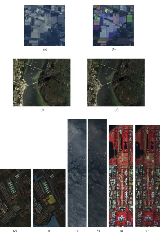
For our experiments, we utilizefive commonly used HSI data sets acquired with different imaging spectroscopy sensors, and from different sites: Kennedy Space Center (KSC) (Ham et al.2005), Indian Pines (Landgrebe2003), Washington DC Mall (DC) (Landgrebe 2003), Okavango Delta, Botswana (Botswana) (Ham et al.2005), and University of Pavia (Uni. of Pavia) (Figure 3).
Indian Pines is a data set of a mixed forest and agricultural land in northwest Indiana. It was acquired in June 1992 using the National Aeronautics and Space Administration (NASA) Airborne Visible/Infrared Imaging Spectrometer (AVIRIS), mounted on an aircraft andflown at about 20 km altitude. It contains 220 spectral bands in wavelength range 0.4–2.5 µm, with a spectral resolution of 10 nm and a geometrical resolution of approximately 20 m per pixel. The entire scene consists of 145145 pixels and there are 16 land-cover classes.
Kennedy Space Center data (614512 pixels) were captured over the KSC site, Florida, in March 1996 as part of NASA’s AVIRIS project. These consist of 224 bands with a spectral resolution of 10 nm in the wavelength range 0.4–2.5 µm. Only 176 bands were used in the analysis after removing those with a low signal-to-noise ratio and water absorption bands. The data were acquired from an altitude of approximately 20 km and have a geometrical resolution of 18 m per pixel. There are in total 13 classes of various land-cover type identified for classification purposes.
The University of Pavia data set was collected using the Reflective Optics System Imaging Spectrometer (ROSIS) hyperspectral sensor of the German national aerospace agency. It is an urban scene (340610 pixels) of the campus of University of Pavia. The
original data are composed of 115 spectral bands ranging from 0.43 to 0.86 µm and with a spectral resolution of 4 nm. Several bands were discarded due to noise, leaving an image with 103 bands in total. The geometrical resolution is 1.3 m per pixel and there are nine land-cover classes identified on the university campus.
(a) (b)
(c) (d)
(e) (f) (g) (h) (i) (j)
Figure 3.HSI data sets. RGB compositions and overlays of the ground truth of the land-cover classes: Indian Pines (a, b), KSC (c, d), University of Pavia (e, f), Botswana (g, h), Washington DC Mall (i, j).
The Botswana data set (2561476 pixels) was acquired over a 7.7 km strip of the Okavango Delta, Botswana, in May 2001 using the hyperspectral sensor of NASA’s Earth Observing-1 satellite. It consists of 242 bands in the wavelength range 0.4–2.5 µm. The geometrical resolution is 30 m per pixel and the spectral resolution is 10 nm. Only 145 bands of the original hyperspectral data were retained after removal of uncalibrated and noisy bands. The data consist of observations of 14 identified classes representing different swamp and drier woodland areas in the delta.
The Washington DC Mall data set (3071280 pixels) is a HSI data set captured over an urban site. It consists of 210 spectral bands in the 0.4–2.4 µm range of the electro-magnetic spectrum. After removal of water absorption channels, 191 bands remained from the original data. Seven land-cover classes were identified for the classification task.
5. Experimental results
We used the five HSI scenes described in Section 4 for our experiments. For ready comparison of the effectiveness of the proposed method, we adopted the experimental set-up of Liao et al. (2013). Specifically, each data set (see Table 1) was partitioned by Table 1.HSI data sets used in the experiments.
Indian Pines KSC
Class no. Class name Count Class name Count
1 Alfalfa 54 Scrub 761
2 Corn no-till 1434 Willow swamp 243
3 Corn minimum-till 834 Cabbage palm hammock 256 4 Corn 234 Cabbage palm/oak hammock 252
5 Grass-pasture 497 Slash pine 161
6 Grass-trees 747 Oak/broadleaf hammock 229 7 Grass-pasture-mowed 26 Hardwood swamp 105 8 Hay-windrowed 489 Graminoid marsh 431
9 Oats 20 Spartina marsh 520
10 Soybeans no-till 968 Cattail marsh 404 11 Soybeans minimum-till 2468 Salt marsh 419 12 Soybeans clean-till 614 Mudflats 503
13 Wheat 212 Water 927
14 Woods 1294
15 Buildings-grass-trees-drives 380 16 Stone-steel-towers 95
Total 10 366 5211
Uni. of Pavia Botswana DC
Class no. Class name Count Class name Count Class name Count
1 Asphalt 6631 Water 270 Roof 3834
2 Meadows 18 649 Hippo grass 101 Street 416 3 Gravel 2099 Floodplain grasses1 251 Path 175 4 Trees 3064 Floodplain grasses2 215 Grass 1928 5 Metal sheets 1345 Reeds1 269 Trees 405 6 Bare soil 5029 Riparian 269 Water 1224 7 Bitumen 1330 Firescar2 259 Shadow 97 8 Self-blocking-bricks 3682 Island interior 203
9 Shadow 947 Acacia woodlands 314
10 Acacia shrublands 248 11 Acacia grasslands 305 12 Short mopane 181 13 Mixed mopane 268 14 Exposed soils 95 Total 42 776 3248 8079
selecting samples uniformly at random such that 70% of the samples were used for training and the remainder comprising a test set. Only in the case of the University of Pavia data set, due to the large number of samples compared with the other data sets, we selected 10,000 samples uniformly at random and partitioned the subsampled data set into 70% training set and 30% testing set. In order to evaluate the method under a low number of training samples, we repeated the experiments for each data set using 10% of the samples (per class) for training and the remaining 90% as a test set.
In both cases we used the training set data without the labels to train one of the spectral sub-feature learning algorithms. Then, after applying the learned feature map-ping, a linear SVM classifier was trained using the transformed training set together with the corresponding labels. Fourfold cross-validation was used to optimize model para-meters. Finally, the model with the optimal parameters was evaluated using the test set. For the two feature learning algorithms, we evaluated the effect of different para-meter values on classification accuracy. Namely, we varied the size of the learned dictionary D, the width w of the convolutional sampling window, the step-size s between consecutive windows, and the number of pooling blocks (Figure 4). Due to the computational constraints of a full grid search over all parameters, each parameter was optimized while keeping the rest fixed. The optimal parameter values were then used to train thefinal model, which was evaluated on the test set.
(b) (a)
(d) (c)
Figure 4.Effects of parameter dictionary size (a), window width (b), step-size (c), and number of pooling blocks (d) for the Indian Pines data set.
In the case of the algorithm based on sparse modelling, there is an additional parameter,λ, which is the sparsity regularization parameter. Since there is no analytical link betweenλand effective sparsity, we tested different numbers of basis vectors using orthogonal matching pursuit (OMP) (Cai and Wang2011) within the set {2, 4, 6, 8, 10, 12, 14, 16, 18, 20, 40, 60, 80, 100, 200, 400}, and used the optimal parameter for each data set.
From the experimental results shown in Figure 4 (similar experimental results for the data sets not included in Figure 4 can be found in the supplementary material https://goo.gl/qwV5F9), it can be seen that over all data sets, and for both dictionary learning algorithms, better results were achieved when using dense convolutional sampling (lower step size) and a higher number of pooling blocks. The convolutional sampling with lower step-sizes allows for a more extensive representation of the input. While pooling is necessary to reduce the size of the final feature vectors, the high number of pooling blocks contributes to preserving the discriminative proper-ties of the features. Therefore, we can make an informed decision for these two parameters without defaulting to cross-validation for their estimation. Considering the effects of the dictionary size parameter when using the SGDk-means dictionary learning algorithm, larger, over-complete dictionaries give better results. On the other hand, when using sparse modelling to learn the dictionary, smaller-size dic-tionaries can perform better than over-complete dicdic-tionaries. The window width parameter also appears to require cross-validation. Considering the effects of this parameter, however, we can see that improvements in the results can be achieved when using large convolutional sampling windows relative to the total number of spectral bands available. However, note that convolutional sampling plays an impor-tant role in the accuracy of both dictionary learning algorithms. Namely, when setting the window width to the total number of spectral bands (effectively disabling convolutional sampling), the classification accuracy drops significantly.
We compare our final test set results to the highest-classification accuracy results reported by Liao et al. (2013) (seeTable 2) using a number of different unsupervised and semi-supervised methods: PCA, NPE, LPP, LLTSA, SDA, SELF, and SELD using NPE as the unsupervised component. Considering the results shown inTable 2, it can be seen that the proposed method outperforms other unsupervised methods on all data sets and achieves better, or as good, results compared to semi-supervised methods.
Table 3shows the classification results of the method when using 10% of the samples from each class for training. The results show that the proposed method produces discriminative features even in cases of low numbers of training samples. Although supervised methods (e.g. simultaneous OMP (SOMP) (Chen, Nasrabadi, and Tran 2011)) can generally provide higher classification accuracies, in some cases, such as the University of Pavia data set, better results can be achieved by the proposed method (cf.Table 3). Therefore, combining the advantages of supervised learning methods and incorporating spatial context information in the proposed approach could provide an interesting topic for future research.
Recently, deep learning models (Krizhevsky, Sutskever, and Hinton2012; Hinton and Salakhutdinov2006) have been successfully used to learn a hierarchical representation of features, where each additional layer of the model represents a higher level repre-sentation of the data. Therefore, we also investigated extensions of our model
architecture with several layers, by applying the unsupervised learning algorithms to the transformed feature representations produced by a previous layer. However, the increase in classification accuracy that we observed was lower than the standard error of the achieved classification scores, which did not justify the additional computational cost incurred by the deep version of our model.
6. Conclusion
In this study we propose an unsupervised spectral sub-feature learning method for classifi ca-tion of hyperspectral images. Experimental results performed on different HSI data sets have shown that the proposed method compares favourably with other unsupervised approaches in HSI classification. Compared to the best results achieved by unsupervised methods in the experiments, our method yields a maximal improvement in overall classification accuracy of up to 12.79%, and an average improvement over all test data sets of 4.22%. Additionally, even Table 2.Comparison of the overall classification accuracy of different methods for HSI classification. For each data set, 70% of the samples are used for training, and the remaining 30% comprises the test set. For the proposed method, the mean overall accuracy (OA) overfive runs is shown together with the standard deviation, as well as the average classification accuracy (AA).
Data sets
Feature extraction Indian Pines KSC Botswana DC Uni. of Pavia Unsupervised methods PCA (%) 73.6 89.6 94 99.7 / NPE (%) 75.7 91.6 94.5 99.7 / LPP (%) 75.1 92 93 99.6 / LLTSA (%) 75.3 90.8 93.5 99.7 / Our method Sparse modelling OA (%) 78.72 ± 0.91 93.89 ± 0.63 89.83 ± 4.67 99.88±0.08 85.91 ± 1.67 Sparse modelling AA (%) 74.92 ± 1 89.92 ± 1.11 90.51 ± 4.52 99.23 ± 0.64 82.64 ± 2.83 SGDk-means OA (%) 88.49±0.33 95.26±0.4 95.16±1.12 99.88±0.03 90.35 ± 0.17 SGDk-means AA (%) 90.1 ± 0.71 92.47 ± 0.61 95.6 ± 0.96 99.62 ± 0.22 86.59 ± 0.21 Semi-supervised methods SDA (%) 65.5 89.8 93.9 99.3 / SELF (%) 73.6 89.6 94 99.7 / SELDNPE(%) 79.2 93.6 95.1 99.8 /
Note: Thefigures in bold represent the highest overall classification scores.
Table 3.Classification accuracy of the proposed method when using only 10% of the samples in the data set for training. The mean overall accuracy (OA) and average accuracy (AA) overfive runs are shown, together with the standard deviation. The overall and average classification accuracies are also shown when using the raw spectral data with no feature extraction.
Data sets
Feature extraction Indian Pines KSC Botswana DC Uni. of Pavia Raw OA (%) 68.89 80.24 81.32 97.4 77.32 Raw AA (%) 55.82 72.01 80.99 87 58.91 Our method Sparse modelling OA (%) 74.27 ± 2.77 86.91 ± 3.53 77.07 ± 5.36 99.56 ± 0.21 74.6 ± 1.62 Sparse modelling AA (%) 64.35 ± 6.35 80.38 ± 4.22 77.38 ± 5.62 96.96 ± 1.3 64.29 ± 2.48 SGDk-means OA (%) 78.96 ± 0.82 90.61 ± 0.27 85.01 ± 1.29 99.6 ± 0.1 86.92 ± 0.39 SGDk-means AA (%) 71.56 ± 0.93 86.57 ± 0.26 85.99 ± 1.15 96.44 ± 0.93 81.63 ± 0.87
though our algorithm uses no labelled data or prior knowledge to learn features, it can achieve similar or better performance than state-of-the-art semi-supervised methods on the same task. Even though recent supervised methods for HSI classification generally outper-form unsupervised and semi-supervised approaches, our method has demonstrated useful properties on certain data sets, which supports future work in combining supervised meth-ods with our approach. Furthermore, the ability of the proposed method to fully exploit the information present in the spectral domain is of importance in hyperspectral data analysis: namely for the classification of materials in spectral libraries, where methods that make use of spatial or geometrical context information cannot be applied. Finally, spectral sub-feature learning can be useful in frameworks, such as that proposed by Li et al. (2015), which integrate multiple types of feature for classification of hyperspectral images.
Disclosure statement
No potential conflict of interest was reported by the authors.
Funding
The research activities described in this article were funded by Ghent University and the Interdisciplinary Research Institute iMinds.
References
Arthur, D., and S. Vassilvitskii. 2007. “K-Means++: The Advantages of Careful Seeding.” In
Proceedings of the 18th Annual ACM-SIAM Symposium on Discrete Algorithms, New Orleans, Louisiana. SODA ’07, 1027–1035. Philadelphia, PA: Society for Industrial and Applied Mathematics.
Bandos, T. V., L. Bruzzone, and G. Camps-Valls.2009.“Classification of Hyperspectral Images with Regularized Linear Discriminant Analysis.”IEEE Transactions on Geoscience and Remote Sensing
47 (3): 862–873. doi:10.1109/TGRS.2008.2005729.
Belkin, M., and P. Niyogi.2001.“Laplacian Eigenmaps and Spectral Techniques for Embedding and Clustering.” In NIPS, edited by T. G. Dietterich, S. Becker, and Z. Ghahramani, 585–591. Cambridge, MA: MIT Press.
Benediktsson, J. A., J. A. Palmason, and J. R. Sveinsson.2005.“Classification of Hyperspectral Data from Urban Areas Based on Extended Morphological Profiles.”IEEE Transactions on Geoscience and Remote Sensing43 (3): 480–491. doi:10.1109/TGRS.2004.842478.
Cai, D., X. He, and J. Han. 2007. “Semi-Supervised Discriminant Analysis.”In Proceedings of the International Conference on Computer Vision(ICCV), Rio de Janeiro, October 1–7. IEEE.
Cai, T. T., and L. Wang.2011.“Orthogonal Matching Pursuit for Sparse Signal Recovery with Noise.”
IEEE Transactions on Information Theory57 (7): 4680–4688. doi:10.1109/TIT.2011.2146090. Castrodad, A., Z. Xing, J. B. Greer, E. Bosch, L. Carin, and G. Sapiro.2011.“Learning Discriminative
Sparse Representations for Modeling, Source Separation, and Mapping of Hyperspectral Imagery.” IEEE Transactions on Geoscience and Remote Sensing 49 (11): 4263–4281. doi:10.1109/TGRS.2011.2163822.
Chang, C.-I., Q. Du, T.-L. Sun, and M. L. G. Althouse.1999.“A Joint Band Prioritization and Band-Decorrelation Approach to Band Selection for Hyperspectral Image Classification.” IEEE Transactions on Geoscience and Remote Sensing37 (6): 2631–2641. doi:10.1109/36.803411. Charles, A. S., B. A. Olshausen, and C. J. Rozell.2011.“Learning Sparse Codes for Hyperspectral
Imagery.” Selected Topics in Signal Processing, IEEE Journal of 5 (5): 963–978. doi:10.1109/ JSTSP.2011.2149497.
Chen, S., and D. Zhang.2011.“Semisupervised Dimensionality Reduction with Pairwise Constraints for Hyperspectral Image Classification.”IEEE Geoscience and Remote Sensing Letters8 (2): 369– 373. doi:10.1109/LGRS.2010.2076407.
Chen, Y., X. Zhao, and X. Jia.2015.“Spectral-Spatial Classification of Hyperspectral Data Based on Deep Belief Network.” Selected Topics in Applied Earth Observations and Remote Sensing, IEEE Journal of PP99: 1–12.
Chen, Y., N. M. Nasrabadi, and T. D. Tran. 2011. “Hyperspectral Image Classification Using Dictionary-Based Sparse Representation.”IEEE Transactions on Geoscience and Remote Sensing
49 (10): 3973–3985. doi:10.1109/TGRS.2011.2129595.
Chen, Y., Z. Lin, X. Zhao, G. Wang, and Y. Gu. 2014. “Deep Learning-Based Classification of Hyperspectral Data.” Selected Topics in Applied Earth Observations and Remote Sensing, IEEE Journal of7 (6): 2094–2107. doi:10.1109/JSTARS.2014.2329330.
Coates, A., and A. Ng.2011.“The Importance of Encoding versus Training with Sparse Coding and Vector Quantization.”InProceedings of the 28th International Conference on Machine Learning, Bellevue, Washington, USA. ICML’11, 921–928. New York, NY: ACM. June.
Coates, A., A. Y. Ng, and H. Lee. 2011. “An Analysis of Single-Layer Networks in Unsupervised Feature Learning.”Journal of Machine Learning Research - Proceedings Track15: 215–223. Ham, J., Y. Chen, M. M. Crawford, and J. Ghosh. 2005. “Investigation of the Random Forest
Framework for Classification of Hyperspectral Data.” IEEE Transactions on Geoscience and Remote Sensing43 (3): 492–501. doi:10.1109/TGRS.2004.842481.
He, X., D. Cai, S. Yan, and H.-J. Zhang.2005.“Neighborhood Preserving Embedding.”InProceedings of the International Conference on Computer Vision (ICCV), October, Vol. 21208–21213. IEEE Computer Society.
He, X., and P. Niyogi.2004.“Locality Preserving Projections.”InNIPS, edited by S. Thrun, L. K. Saul, and B. Schölkopf, 153–160. MIT Press.
Hinton, G., and R. Salakhutdinov. 2006. “Reducing the Dimensionality of Data with Neural Networks.”Science313 (5786): 504–507. doi:10.1126/science.1127647.
Hinton, G. E., S. Osindero, and Y.-W. Teh.2006.“A Fast Learning Algorithm for Deep Belief Nets.”
Neural Computation18 (7): 1527–1554. doi:10.1162/neco.2006.18.7.1527.
Hotelling, H. 1933. “Analysis of a Complex of Statistical Variables into Principal Components.”
Journal of Educational Psychology24 (6): 417–441. doi:10.1037/h0071325.
Huang, H.-Y., and B.-C. Kuo. 2010. “Double Nearest Proportion Feature Extraction for Hyperspectral-Image Classification.” IEEE Transactions on Geoscience and Remote Sensing 48 (11): 4034–4046.
Hughes, G.1968.“On the Mean Accuracy of Statistical Pattern Recognizers.”IEEE Transactions on Information Theory14 (1): 55–63. doi:10.1109/TIT.1968.1054102.
Hyvärinen, A., and E. Oja.2000.“Independent Component Analysis: Algorithms and Applications.”
Neural Networks13 (4–5): 411–430. doi:10.1016/S0893-6080(00)00026-5.
Ji, R., Y. Gao, R. Hong, Q. Liu, D. Tao, and L. Xuelong. 2014. “Spectral-Spatial Constraint Hyperspectral Image Classification.” IEEE Transactions on Geoscience and Remote Sensing 52 (3): 1811–1824. doi:10.1109/TGRS.2013.2255297.
Kaewpijit, S., J. Le-Moigne, and T. El-Ghazawi. 2003. “Automatic Reduction of Hyper-Spectral Imagery Using Wavelet Spectral Analysis.”IEEE Transactions on Geoscience and Remote Sensing
41 (4): 863–871. doi:10.1109/TGRS.2003.810712.
Krizhevsky, A., I. Sutskever, and G. E. Hinton. 2012. “ImageNet Classification with Deep Convolutional Neural Networks.” In Advances in Neural Information Processing Systems 25: 1097–1105.
Kuo, B.-C., H.-H. Ho, C.-H. Li, C.-C. Hung, and J.-S. Taur.2014.“A Kernel-Based Feature Selection Method for SVM with RBF Kernel for Hyperspectral Image Classification.”IEEE Journal of Selected Topics in Applied Earth Observations and Remote Sensing 7 (1): 317–326. doi:10.1109/ JSTARS.2013.2262926.
Kuo, B.-C., and D. A. Landgrebe. 2004. “Nonparametric Weighted Feature Extraction for Classification.” IEEE Transactions on Geoscience and Remote Sensing 42 (5): 1096–1105. doi:10.1109/TGRS.2004.825578.
Landgrebe, D. A. 2003. Signal Theory Methods in Multispectral Remote Sensing. Wiley series in remote sensing. Hoboken, N.J., Chichester: Wiley.
Lee, H., A. Battle, R. Raina, and A. Y. Ng.2006.“Efficient Sparse Coding Algorithms.”InNIPS, edited by B. Schölkopf, J. C. Platt, and T. Hoffman, 801–808. MIT Press.
Lee, H., R. Grosse, R. Ranganath, and A. Y. Ng. 2009. “Convolutional Deep Belief Networks for Scalable Unsupervised Learning of Hierarchical Representations.” In Proceedings of the 26th Annual International Conference on Machine Learning, Montreal, Quebec, Canada. ICML ’09, 609–616. New York, NY: ACM.
Li, C.-H., H.-S. Chu, B.-C. Kuo, and C.-T. Lin.2011.“Hyperspectral Image Classification Using Spectral and Spatial Information Based Linear Discriminant Analysis.”InIEEE International Geoscience and Remote Sensing Symposium(IGARSS), July, 1716–1719. IEEE.
Li, J., and Y. Qian. 2011. “Dimension Reduction of Hyperspectral Images with Sparse Linear Discriminant Analysis.” In IEEE International Geoscience and Remote Sensing Symposium
(IGARSS), July, 2927–2930. IEEE.
Li, J., X. Huang, P. Gamba, J. M. Bioucas-Dias, L. Zhang, J. A. Benediktsson, and A. Plaza.2015.
“Multiple Feature Learning for Hyperspectral Image Classification.” IEEE Transactions on Geoscience and Remote Sensing53 (3): 1592–1606. doi:10.1109/TGRS.2014.2345739.
Liao, W., A. Pizurica, P. Scheunders, W. Philips, and P. Youguo. 2013. “Semisupervised Local Discriminant Analysis for Feature Extraction in Hyperspectral Images.” IEEE Transactions on Geoscience and Remote Sensing51 (1): 184–198. doi:10.1109/TGRS.2012.2200106.
Mairal, J., F. Bach, J. Ponce, and G. Sapiro.2009.“Online Dictionary Learning for Sparse Coding.”In
Proceedings of the 26th Annual International Conference on Machine Learning, Montreal, Quebec, Canada. ICML’09, 689–696. New York, NY: ACM.
Qiao, L., S. Chen, and X. Tan. 2010. “Sparsity Preserving Projections with Applications to Face Recognition.”Pattern Recognition43 (1): 331–341. doi:10.1016/j.patcog.2009.05.005.
Roweis, S. T., and L. K. Saul. 2000. “Nonlinear Dimensionality Reduction by Locally Linear Embedding.”Science290 (5500): 2323–2326. doi:10.1126/science.290.5500.2323.
Sculley, D. 2010. “Web-Scale K-Means Clustering.” In Proceedings of the 19th International Conference on World Wide Web, Raleigh, North Carolina, USA. WWW ’10, 1177–1178. New York, NY: ACM.
Shao, Z., and L. Zhang.2014.“Sparse Dimensionality Reduction of Hyperspectral Image Based on Semi-Supervised Local Fisher Discriminant Analysis.” International Journal of Applied Earth Observation and Geoinformation31: 122–129. doi:10.1016/j.jag.2014.03.015.
Sugiyama, M. 2007. “Dimensionality Reduction of Multimodal Labeled Data by Local Fisher Discriminant Analysis.”Journal Mach Learning Researcher8: 1027–1061.
Sugiyama, M., T. Idé, S. Nakajima, and J. Sese.2010.“Semi-Supervised Local Fisher Discriminant Analysis for Dimensionality Reduction.”Machine Learning78 (1–2): 35–61. doi: 10.1007/s10994-009-5125-7.
Sun, X., Q. Qu, N. M. Nasrabadi, and T. D. Tran.2014.“Structured Priors for Sparse-Representation-Based Hyperspectral Image Classification.” IEEE Geoscience and Remote Sensing Letters11 (7): 1235–1239. doi:10.1109/LGRS.2013.2290531.
Tao, C., J. Jin, Y. Tang, and Z. Zou.2013.“Hyperspectral Imagery Classification Based on Rotation Invariant Spectral-Spatial Feature.” In IEEE International Geoscience and Remote Sensing Symposium(IGARSS), July, 422–424. IEEE.
Tenenbaum, J. B., V. de Silva, and J. C. Langford. 2000. “A Global Geometric Framework for Nonlinear Dimensionality Reduction.” Science 290 (5500): 2319–2323. doi:10.1126/ science.290.5500.2319.
Tuia, D., M. Volpi, M. Dalla Mura, A. Rakotomamonjy, and R. Flamary. 2014.“Automatic Feature Learning for Spatio-Spectral Image Classification with Sparse SVM.” IEEE Transactions on Geoscience and Remote Sensing52 (10): 6062–6074. doi:10.1109/TGRS.2013.2294724.
Wang, J., and C.-I. Chang. 2006. “Independent Component Analysis-Based Dimensionality Reduction with Applications in Hyperspectral Image Analysis.”IEEE Transactions on Geoscience and Remote Sensing44 (6): 1586–1600. doi:10.1109/TGRS.2005.863297.
Wang, J., J. Yang, K. Yu, F. Lv, T. S. Huang, and Y. Gong.2010.“Locality-Constrained Linear Coding for Image Classification.”InCVPR, 3360–3367. IEEE Computer Society.
Yang, J., K. Yu, Y. Gong, and T. S. Huang.2009.“Linear Spatial Pyramid Matching Using Sparse Coding for Image Classification.”InCVPR, 1794–1801. IEEE Computer Society.
Yang, S., H. Jin, L. Yang, W. Xu, and L. Jiao. 2014. “Compressive Sensing-Inspired Dual-Sparse SLFNN for Hyperspectral Imagery Classification.”IEEE Geoscience and Remote Sensing Letters11 (1): 220–224. doi:10.1109/LGRS.2013.2253443.
Zhang, L., L. Zhang, D. Tao, and X. Huang. 2012. “On Combining Multiple Features for Hyperspectral Remote Sensing Image Classification.” IEEE Transactions on Geoscience and Remote Sensing50 (3): 879–893. doi:10.1109/TGRS.2011.2162339.
Zhang, L., Q. Zhang, L. Zhang, D. Tao, X. Huang, and D. Bo.2015.“Ensemble Manifold Regularized Sparse Low-Rank Approximation for Multiview Feature Embedding.”Pattern Recognition48 (10): 3102–3112. doi:10.1016/j.patcog.2014.12.016.
Zhang, T., J. Yang, D. Zhao, and X. Ge. 2007. “Linear Local Tangent Space Alignment and Application to Face Recognition.” Neurocomputing 70 (7–9): 1547–1553. doi:10.1016/j. neucom.2006.11.007.
Zhang, Z., and H. Zha. 2005. “Principal Manifolds and Nonlinear Dimensionality Reduction via Tangent Space Alignment.”SIAM Journal Sciences Computation 26 (1): 313–338. doi:10.1137/ S1064827502419154.
Zhong, Y., X. Lin, and L. Zhang.2014.“A Support Vector Conditional Random Fields Classifier with A Mahalanobis Distance Boundary Constraint for High Spatial Resolution Remote Sensing Imagery.”IEEE Journal of Selected Topics in Applied Earth Observations and Remote Sensing 7 (4): 1314–1330. doi:10.1109/JSTARS.4609443.