multi-objective particle swarm optimisation
Jonathan E. Fieldsend
School of Engineering, Computing and Mathematics, University of Exeter,
Harrison Building, North Park Road, Exeter, EX4 4QF, UK. [email protected]
Summary. Although conceptually quite simple, decision trees are still amongst the most popular classifiers applied to real-world problems. Their popularity is due to a number of factors – core amongst these is their ease of comprehension, robust performance and fast data processing capabilities. Additionally feature selection is implicit within the decision tree structure.
This chapter introduces the basic ideas behind decision trees, focusing on deci-sion trees which only consider a rule relating to a single feature at a node (there-fore making recursive axis-parallel slices in feature space to form their classification boundaries). The use of particle swarm optimisation (PSO) to train near optimal decision trees is discussed, and PSO is applied both in a single objective formula-tion (minimising misclassificaformula-tion cost), and multi-objective formulaformula-tion (trading off misclassification rates across classes).
Empirical results are presented on popular classification data sets from the well-known UCI machine learning repository, and PSO is demonstrated as being fully capable of acting as an optimiser for trees on these problems. Results addition-ally support the argument that multi-objectification of a problem can improve uni-objective search in classification problems.
1 Introduction
The problem of classification is a popular and widely confronted one in data-mining, drawing heavily from the fields of machine learning and pattern recognition. Classification, most simply put, is the assignment of a class Ci to some observed datam x, based on some functional transformation of x, ˆ
p(Ci|x) =f(x,s,D), where ˆp(Ci|x) is an estimate of the underlying probabil-ity of observationx belonging to classi (the class typically assigned by the classifier toxbeing that class with the highest estimated probability), andD
is some set of pre-labelled data used in the selection of model parameterss. Depending on the classifier used, it may produce the probability directly, a score that can be converted into a probability, or a hard classification (that is,
assigning all the probability to a single class). The learning (or optimisation) aspect in classifiers relates to s, the tunable parameters of classifier function f().1
These are adjusted so as to minimise the difference between the esti-mated probabilities assigned to data, and the underlying true probabilities. Often the latter are not known, and this has to be approximated using the corpus oftraining dataD, and possibly some prior.
The range of classification problems is extensive, with applications as di-verse economics and finance, biology, engineering and safety systems, medicine, etc. One of the most popular classifiers (if notthe most popular) is the deci-sion tree [2]. A decideci-sion tree consists of a sequence of connected nodes, each of which act as a discriminator. The edges between the nodes are uni-directional, and travelling down from the root node, they act to sequentially partition the data space until a terminus node (also known as a leaf) is reached. The leaf as-signs a class (or infrequently a pseudo class probability) to the unique volume of feature space covered by the leaf. The internal nodes themselves partition the data by applying a rule to the data, typically these are of the form ‘if-then-else’. For instance, the rule may be ‘if feature 2 is greater than 2.5, go to child node 1, else go to child node 2’. This feature may for instance be the age of an individual or the amount of money applied for in a loan – and the child nodes may contain further rules, or be leaf nodes relating to actual decisions. Decision trees derive a lot of their popularity from their ease of compre-hension. The assignment of class can be traced back to a sequence of rules, which make it easy to explain to end users; this also aids tremendously in their application to e.g. safety critical systems [3] or medical applications [4], where ‘black box’ classifiers have difficulty passing regulatory hurdles due to their opaque processing nature. Additionally their computational complexity is relatively low and are ideally specified for batch processing, meaning they are widely used for real-time classification tasks, and problems requiring a large throughput of data.
The chapter will proceed as follows, in Section 2 decision trees will be discussed in further depth along with their properties. In Section 3 the ba-sic particle swarm optimisation (PSO) algorithm is introduced, followed by Section 4 which discusses the representation of decision trees to enable opti-misation by PSO. Section 5 discusses various multi-objective problems related to decision trees, and introduces a multi-objective PSO variant to optimise decision trees. Section 6 presents empirical results using the most popular data sets from the widely used UCI machine learning repository [5], with a chapter summary presented in Section 7.
1
It sometimes also relates to choosing f(), or to selecting the most informative members of D to learn from (data which can also form a part of s in some classifiers, e.g. k-nearest neighbours and support vector machines [1]).
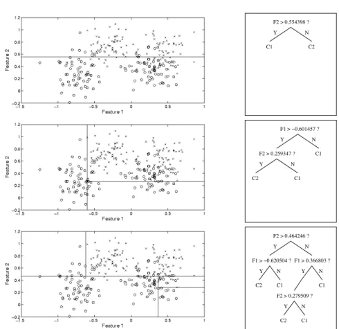
C2 C1 F2 > 0.554398 ? Y N C2 C1 F1 > −0.601457 ? Y N F2 > 0.259347 ? Y N C1 F1 > 0.366803 ? F2 > 0.464246 ? Y N F1 > −0.620504 ? C1 C2 C1 Y N Y N C2 C1 N Y F2 > 0.279509 ?
Fig. 1.Left: Decision tree partitioning of the Ripley data feature space, minimising total misclassification (class 1 data denoted by circles, class 2 by crosses). Right: Corresponding trees.
2 Decision trees
As mentioned in the preceding section, the nodes in a decision tree act as rules, recursively partitioning the decision space. If the rule covers a single feature, as the example given above, then the partitions are axis parallel2
, although this generates quite a simple decision boundary, as the tree depth is increased the feature space can be partitioned into more and more different sections, and the resulting decision boundary becomes more complex (though piecewise linear, and axis parallel in these sections).
2
Some decision trees also combine features in single rules, enabling non-axis-parallel partitions of feature space. This form will not be covered further here however.
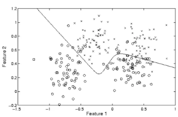
Fig. 2. Bayes rule decision boundary on the synthetic Ripley data (the best pos-sible decision boundary, assuming equal misclassification costs, generated from the underlying data model).
Figure 1 shows example decision tree decision boundaries (and correspond-ing trees) for the two dimensional synthetic data from [6]3
. Note that the trees shown are of various depths, illustrating the way the decision boundary com-plexity can increase with tree depth. The corresponding Bayes rule decision boundary for this problem is shown in Figure 2 for completeness.
Amongst the most popular traditional learning algorithms for decision trees are CART (classification and regression trees) [7], ID3 (iterative di-chotomiser 3) [8] and C4.5 [9]. The search through all the possible symbol choices for a symbol (the rule or class to contain in a node), along with all possible thresholds is typically infeasible (irrespective of the computational cost of varying the depth of the tree). As such tree learning algorithms typi-cally employ some form of greedy search, performing a local exhaustive search at the data covered by a node when selecting its symbol and threshold. The issue of when to stop growing the tree (make a node a terminal) is be con-fronted in a number of approaches, by stopping the growth when the reduction in prediction error (typically entropy is used) falls below a certain threshold, when the number of points covers by a node falls below a certain threshold, or letting a tree grow large and then prune back (remove and recombine) leafs, based on some trade-offof accuracy (error) and complexity (tree size).
Given the nature of the tree learning/optimisation (its size and complex-ity), and that the learning methods currently used are only locally optimal, evolutionary optimisation algorithms have also gained popularity as decision tree parameter optimisers.
3
This data is generated by sampling from four two-dimensional Gaussians, with centres of class 1 instances at µ11 = (−0.7,0.3),µ12 = (0.3,0.3) and centres of
class 2 instances atµ21= (−0.3,0.7),µ22= (0.4,0.7), with identical covariances
3 Particle swarm optimisation
The PSO heuristic was initially proposed for the optimisation of continuous non-linear functions [10]. Subsequent work in the field has developed some methods for its operation in discrete domains (e.g. [11]) however the contin-uous domain remains its principle field of deployment.
In standard PSO a fixed population ofM potential solutions, {si}M i=1, is
maintained, where each of these solutions (or particles) is represented by a point inP-dimensional space (whereP is the number of parameters to be op-timised). Each of these solutions maintains knowledge of its ‘best’ previously evaluated position (its personal best) pi, and also has access to the ‘best’ solution found so far by the population as a whole, g, which by definition is also one of the swarm member’s personal best. The rate of position change of a particle/solution from one iteration/generation to the next depends upon its previous local best position, the global best position, and its previous tra-jectory (its velocity,vi). The general formula for adjusting thejth parameter of theith particle’s velocity is:
vj,i:=wvj,i+c1r1(pj,i−sj,i) +c2r2(gj−sj,i) (1)
sj,i:=sj,i+χvj,i. (2)
Where w, c1, c2, χ ≥ 0. w is the inertia of a particle (how much its
previous velocity affects its next trajectory),c1 andc2 are constraints on the
velocity toward the global and local best andχis a constraint on the overall shift in position (often a maximum absolute velocity, Vmax is also applied).
r1andr2 are random draws from the continuous uniform distribution, i.e.r1,
r2 ∼U(0,1). In [10] the final model presented hasw and χ fixed at 1, and
c1 andc2 fixed at 2. Later work has tended toward varying the inertia term
downward during the search to aid final convergence.
The PSO heuristic has proved to be an extremely popular optimisation technique, with reputation for relatively fast convergence, and as such is its application to decision tree optimisation has recently gained interest.
4 Representation
As you may have noted from the description above, decision trees may be variable in size, with their parameters a mixture of unordered discrete (i.e. which features and rules to include in nodes, and which class to assign to a leaf) and ordered continuous (i.e. which thresholds to use in rules). As such the evolutionary algorithm of choice for optimising them has tended to be genetic algorithms (see e.g. [12] for a recent discussion of these methods in a multi-objective setting). Heuristic tree growing and pruning methods are
14
0
1
2
3
4
5
6
7
8
9
10
11
12
13
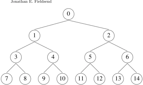
Fig. 3. Illustration of a fullA-ary tree withLlayers, whereA=2 andL=3.
amongst the more traditional forms of decision tree construction [2], as dis-cussed in Section 2, and advanced methods from the machine learning liter-ature like Bayesian averaging have also been applied [13] (although it is an open problem to effectively sample from the posterior). Recently Veenhuiset al. [14] introduced a general PSO-based ‘tree swarming algorithm’ for opti-mising generic tree structures (i.e. decision trees, parse tress, program trees, etc) with respect to a single quality (objective) measure. A slightly modified version of their tree representation is used here, and is described below (with variations from [14] highlighted).
Figure 3 illustrates a full ordered 2-ary tree with a single root, 4 layers and directed edges (denoted byT4,2). As the tree is full, the final layer (nodes
7-14) are terminal nodes (leafs), having no children of there own. The size of a general tree with Llayers and arity ofA, TL,A, in terms of the number of internal and terminal nodes is
size(TL,A) = L−1
!
i=0
Ai. (3)
(Note also there aresize(TL,A)−1 edges in a full TL,A tree.)
Although trees may be mapped to a continuous valued vector for use in Equation 1, it is easier for comprehension to describe the mapping in terms of a continuous valued matrix (the final transformation from a matrix to a vector representation being trivial). First consider the mapping of the nodes in a tree to an array. As laid out in [14], and illustrated in Figure 3, the nodes may be numbered in the tree, starting at 0 at the root, and counting from left to right at each subsequent level. The index of a child nodecof any particular parent nodepcan be calculated as:
14
0
1
2
3
4
5
6
7
8
9 10 11 12 13
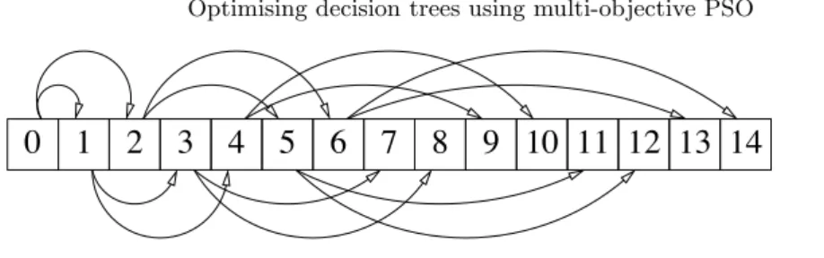
Fig. 4. Illustrative node array.
child index(p, c, A) =Ap+c. (4)
Where c denotes the cth child of parent p (i.e. 1 ≤ c ≤ A), and 0 ≤ p≤size(TL,A)−1. Using Equation 4 one can travel down the tree until the appropriate leaf is reached. Figure 4 shows the node array constructed in this fashion corresponding to the tree in Figure 3.
The representation of node traversal has now been covered, however the key problem is in the transformation of the rules (symbols) to continuous values for use in PSO, which can impose a (variable) order on the symbols. This is confronted by [14] with the use of a symbol vector, whose length is equal to the total number of symbols possible in a node (in the case of decision trees, this would be number of different rules plus the number of different classes). Each element in the symbol vector is a score (here on the range [0,1]), with the symbol used being determined by the index of the element in the symbol vector with the maximum score. Consider for instance a classification problem with five features and three classes, which we want to describe using a tree exclusively using rules of the ‘if feature greater than else’ form. This would lead to eight distinct symbols, the first five relating to which feature to use in the rule, and the last three to which class to assign, i.e. {‘if feature 1 is greater than, else’,‘if feature 2 is greater than, else’, ‘if feature 3 is greater than, else’,‘if feature 4 is greater than, else’,‘if feature 5 is greater than, else’, ‘class 1’, ‘class 2’, ‘class 3’}. A node with a symbol vector whose maximum element was 1, 2, 3, 4, or 5 would be an internal node, whereas one with a maximum element 6, 7 or 8 would be a leaf (note this representation allows the mapping to be used for sparser trees, if the node belongs to a layer< L and is assigned a leaf symbol, then none of that node’s subsequent children will be evaluated).
Using the symbol vector notation, the decision tree can be represented as a matrix of symbol scores, M, with each column denoting a node and each row denoting a symbol, as shown below for aT3,2tree with five symbols.
0 1 2 3 4 5 6 S1 S2 S3 S4 S5 M1,1, M1,2, M1,3, M1,4, M1,5, M1,6, M1,7 M2,1, M2,2, M2,3, M2,4, M2,5, M2,6, M2,7 M3,1, M3,2, M3,3, M3,4, M3,5, M3,6, M3,7 M4,1, M4,2, M4,3, M4,4, M4,5, M4,6, M4,7 M5,1, M5,2, M5,3, M5,4, M5,5, M5,6, M5,7 .
The symbolSi to use for a particular nodej+ 1 being the determined by the maximum element of the jth column ofM. The issue of the threshold is resolved in [14] by making the decision trees 3-ary, with the first element of the symbol vector of the first child of an internal node determining the threshold (by rescaling the value contained from [0,1] to [min(Fi),max(Fi)], where Fi denotes the feature used in the rule, andmin(Fi) and max(Fi) returning the minimum and maximum respectively of feature i in the training data. This is a somewhat wasteful representation as only the first symbol of the first child node will ever be used, and none of its subsequent children will ever be accessed (although they will be represented) as it is treated as a terminal node. The same effect may be implemented with much less space required by adding an extra row on the bottom of matrixM to hold the threshold to be used if the node is internal. An arguably even better approach, is to addzextra rows on the bottom of M (where z is the number of features), so that there are different threshold values represented for each different feature. This allows the thresholds at nodes to be learnt in parallel and prevents the problems that may arise when changing the feature potentially makes the single threshold stored inappropriate. This does increase the number of dimensions of the problem, but should act to improve the smoothness of the search space.
It is worth noting that whereas the matrix representation is easier to inter-pret, there is no reason for it not to be represented in a program as a vector. Conversion between the two representations is trivial, and if a preferred op-timiser is already implemented to deal exclusively with vector represented solutions, this intermediate conversion may be used as an interface between the solution and evaluation.
5 Multi-objective PSO
As discussed above, PSO has previously been applied to single objective de-cision tree optimisation (where total misclassification is the objective to be minimised). There are however situations where one might want to optimise a decision tree with respect to multiple objectives. Three specific situations are covered here. Firstly when also minimising the size of the tree. This may be important due to processing time – the larger the tree the longer the process-ing time for a particular query, which in certain situations may be a critical
factor (e.g., real time fraud detection). Secondly when also minimising the number of features used by the tree. Initial and subsequent feature selection for a classification system has a cost associated with it (sometimes quite sig-nificant, e.g. chemical/biological measurements), minimising the number of features used acts to lower this cost, and also remove any redundancy across features. Thirdly when multiple error measures need to be optimised – for in-stance in binary classification problems the overall misclassification rate may be less important than the relative true and false positive rates, where mis-classification costs are not equal (e.g. cancer detection). A brief outline of these types of multi-objective problem is given below.
5.1 Multiple objectives
Structure
As mentioned in the introduction, one of the attractions of decision trees as classifiers is the fast computation time when classifying new data. The com-putational cost is directly proportional to the number of internal nodes in a tree, and therefore the smaller the tree the faster the processing ability. Addi-tionally there tends to be a trade-offbetween a decision tree’sgeneralisation
ability and size (a tree that is too big – too flexible – may overfit to the data being trained on). This is usually apparent when the number of data samples covered by each leaf is very small (hence the use of pruning in some tree learn-ing algorithms, as mentioned in Section 2). A natural additional objective is therefore to minimise the size of the tree (see for example [12]).
Feature space
In many real world situations data collection costs time and money. Features which don’t contribute to the performance of a classifier can be detrimental if included, and others may duplicate information or have only a marginal effect. As such feature selection, and feature minimisation are also of concern when constructing decision trees, and can also be cast as an additional objective, both as a means of improving generalisation performance, and to decrease the cost of future data collection.
Multiple error terms
By minimising the total misclassification error one is implicitly stating that the misclassification costs across classes are equivalent. Often this is not the case (for example when screening for cancers, or in safety related classifi-cation problems). Where the costs are unknown a priori and/or the shape of the trade-off front is unknown, it is appropriate to trade-off the different misclassification rates in parallel [15, 16]. An illustration of this is provided in Figure 5 using the synthetic data described earlier. The upper right plot
0 10 20 30 40 50 60 70 80 90 100 0 10 20 30 40 50 60 70 80 90 100 Class 1 misclassification % Class 2 misclassification %
Fig. 5. a,c,d) Decision tree partitioning of the Ripley data feature space, trading off misclassifiction rates between the two classes, b) Corresponding points in mis-classification rate space.
shows the objective space mapping of three decision trees, where the objec-tives are minimising the class 1 misclassification rate and minimising the class 2 misclassification rate. Note this is equivalent to the widely used Receiver Operating Characteristic (ROC) curve representation used for binary classi-fication tasks – by representing the curve in terms of both misclassiclassi-fication rates, instead of focusing on a single class (correct assignment and incorrect assignment rates to that class), the problem is more easily extended to mul-tiple (i.e. > 2) class problems [15, 16]. The class mapping on feature space caused by the three mutually non-dominating trees are also plotted in 5, and arranged in the order they are plotted in the trade-offfront.4
5.2 Dominance and Pareto optimality
The vast majority of recent multi-objective optimisation algorithms (MOAs) rely on the properties of dominance and Pareto optimality to compare and judge potential solutions to a problem, as such these will be briefly reviewed here before discussing the multi-objective PSO algorithm.
4
Note that as there is no assessment on a test set of data the generalisation ability of these trees is not indicated (visually we would be concerned of the overfitting of the bottom left tree for instance, given our knowledge of the underlying data generation process).
The multi-objective optimisation problem is concerned with the simulta-neous extremisation ofD objectives:
yi=fi(s), i= 1, . . . , D (5) where each objective evaluation depends upon the parameter vector s= {u1, u2, . . . , uP}. These parameters may also be subject to various inequality
and equality constraints:
ej(s)≥0, j= 1, . . . , J (6) gk(s) = 0, k= 1, . . . , K (7) Without loss of generality it can be assumed that the objectives are to be minimised, thus the problem can be expressed as:
Minimise y=f(s) ={f1(s), f2(s), . . . , fP(s)}, (8) subject to e(s) ={e1(s), e2(s), . . . , eJ(s)}≥0, (9)
g(s) ={g1(s), g2(s), . . . , gK(s)}= 0. (10)
When concerned with a single objective, an optimal solution is one which minimises the objective subject any constraints within the model. In the sit-uation where there is more than one objective, then it is often the case that solutions exist for which performance cannot be improved on one objective without sacrificing performance on at least one other. Such solutions are said to bePareto optimal, with the set of all such solutions being the Pareto set, and their image in objective space known as thePareto front.
The notion of dominance is crucial to understanding Pareto optimality, and is relied upon heavily in most modern multi-objective optimisers. A de-cision vector (also known as a solution/parameter vector)sis said tostrictly dominate anotherv(denoted s≺v) iff
fi(s)≤fi(v), ∀i= 1, . . . , D and (11) fi(s)< fi(v), for at least onei. (12) Note that the dominance relationships≺v is denoted in the parameter space domain, whereas the calculation is in the objective space mapping of the parameters. As suchf(s)≺f(v) is perhaps more accurate, however the accepted shorthand will be used throughout the rest of the chapter.
A set ofN decision vectorswi is said to be anon-dominated set (i.e. and estimate of the Pareto set) if no member of the set is dominated by any other member:
Algorithm 1A multi-objective PSO algorithm.
Require: I Number of PSO iterations
Require: M Number of particles/solutions
Require: N Dimension of search problem
Require: w Inertia value
Require: c1 Global search weight
Require: c2 Local search weight
Require: χ Constriction variable
Require: Vmax Absolute maximum velocity
1: {S,V}:=initialise population(M, N) See Algorithm 2 2: i:= 0
3: Y:=evaluate(S) Assess particle
4: G:=initialise gbest(S, N) See Algorithm 4 5: P:=initialise pbest(S, N) See Algorithm 3 6: whilei < I:do
7: V:=update velocity(S,P,G, w, c1, c2, N) See Algorithm 5
8: V:=restrict velocity(V, Vmax) Ensure no velocity element exceedsVmax
9: P:=S+χV
10: Y:=evaluate(S) Assess particle
11: G:=update gbest(G,S) See Algorithm 7 12: P:=update pbest(P,S) See Algorithm 6 13: w:=update inertia(w, n) Decrease inertia 14: i:=i+ 1
15: end while
wi'≺wj ∀i, j= 1, . . . , M. (13) The aim of most MOAs is to find such a non-dominated set – whose image in objective space is well converged to, and spread across, the true Pareto front, and is therefore a good approximation of the underlying Pareto set.5
5.3 The optimiser
There are a number of different approaches to extending PSO to multi-objective problems (see e.g. [17, 18] for reviews). Building on the previous work of Alvarez-Benitezet al.[19], the implementation used here relies solely on dominance to select the guides for individual particles (although the use of distance measures on search space is also investigated). This circumvents the issue of bias and appropriate objective weighting that other alternative selection processes can lead to [17].
Using the decision tree representation presented earlier, a general multi-objective PSO algorithm is presented in Algorithm 1.
5
Note that due to the non-linear mappings involved, closeness in objective space may not relate to closeness in decision space. As such, even if the Pareto front is known a priori, closeness to it is not a guarantee that the set members are “close” in parameter space to the Pareto set.
Algorithm 2initialise population(M, N).
1: S:= Ø Create empty set
2: V:= Ø Create empty set
3: i:= 1
4: whilei≤M do 5: j:= 1
6: whilej≤N do
7: Si,j:=U(0,1) Insert a uniform sample from (0,1)
8: Vi,j:= 0 Initialise velocity – random samples also possible
9: j:=j+ 1 10: end while 11: i:=i+ 1 12: end while
13: return {S,V} Return initial search population and velocity
Algorithm 3initialise pbest(S, N).
1: i:= 1
2: whilei≤N do
3: Pi:= Ø Create empty personal best set for search particle
4: Pi:=Pi∪Si insert current position as initial set
5: i:=i+ 1 6: end while
7: return P Return personal best sets
Algorithm 4initialise gbest(S, N).
1: G:= Ø Create empty global best set
2: i:= 1
3: whilei≤N do
4: if Si$≺Sj, ∀Sj∈S, i$=jthen
5: G:=G∪Si (If particle non-dominated) add to global best set
6: end if 7: i:=i+ 1 8: end while
9: return G Return global best set
As detailed in Algorithm 1, the principle inputs to the optimiser are the coefficients from Equation 1, along with the number of iterations the optimiser is to be run for (alternatively convergence measures could be used instead [20]), the number of particles in the search population, I, and the solution size, N (which can be calculated from the Equations given in Section 4).
The evaluate() procedure (lines 3 and 9) relies on the transformation of
the solution vector to a tree (as described in Section 4), and the subsequent evaluation on a set of dataDand calculation of errors (examples of which are given in Section 5.1). The search populationS, and associated velocitiesVare initialised using draws from the uniform distribution (line 1, and Algorithm 3),
Algorithm 5update velocity(S,P,G, w, c1, c2, N).
1: i:= 1
2: whilei≤N do 3: j:= 1
4: whilej≤|Si|do
5: r1=U(0,1) Draw from a continuous uniform distribution distribution
6: r2=U(0,1) Draw from a continuous uniform distribution distribution
7: Vi,j=wvi,j+r1c1(get(G,Si)−Si,j) +r2c2(get(Pi,Si, i)−Si,j)
8: j:=j+ 1 (Alter velocity according to Equation 1, see Algorithm 8) 9: end while
10: i:=i+ 1 11: end while
12: return V Return updated velocity
Algorithm 6update pbest(P,S, N).
1: i:= 1
2: whilei≤N do
3: if Si$≺Pij ∀Pij∈Pithen
4: Pi:=Pi∪Si (If particle non-dominated) add to personal best set
5: j:= 1
6: whilej≤|Pi|do 7: if Si≺Pij then
8: Pi:=Pi\Pi
j(If member is dominated) remove from personal best set
9: end if 10: j:=j+ 1 11: end while 12: end if 13: i=i+ 1 14: end while
15: return P Return personal best sets
and after evaluating the search population the global best and personal best vectors are initialised. As discussed in Section 5.2, there is usually no single ‘best’ solution when optimising with respect to more than one objective, and as such a set of mutually non-dominated solutions, which are the best so far encountered by the search population are maintained in G (lines 4 and 10 of Algorithm 1 and Algorithms 4 and 7). Likewise there is likely non single personal best, and a set of setsPis maintained, withPi containing the best set of mutually non-dominating solutions found by particleSiin the search so far (lines 5 and 11 of Algorithm 1 and Algorithms 3 and 6), as used previous in e.g. [21].
The basic PSO update algorithm in Equation 1 is implemented in lines 7-8 of Algorithm 1, with line 7 laid out more fully in Algorithm 5. The key part in Algorithm 5 is line 7 where the get() function is called to return a global best individual and personal best individual respectively. Two different
Algorithm 7update gbest(G,S, N). 1: i:= 1
2: whilei≤N do
3: if Gj$≺Si ∀Gj∈G then
4: G:=G∪Si (If particle non-dominated) add to global best set
5: j:= 1
6: whilej≤|G|do 7: if Si≺Gjthen
8: G:=G\Gj (If member is dominated) remove from global best set
9: end if 10: end while 11: j:=j+ 1 12: end if 13: i=i+ 1 14: end while
15: return G Return global best set
Algorithm 8get(A,s), implementation relying solely on dominance.
1: AS= Ø Initialise empty set of dominating individuals 2: i:= 1
3: whilei≤|A|do 4: if Ai≺s then
5: AS :=AS
∪Ai Add set member that dominatess
6: end if 7: i:=i+ 1 8: end while 9: r:=U(1,|AS
|) Draw from a discrete uniform distribution 10: return ASr Return random dominating individual
implementations of these methods are implemented here. The first method, relying solely on dominance, is laid out in Algorithm 8. Here the selected global best for a solution,Si, is a member ofGwhich dominatesSi (selected at random from the subset ofGwhich dominates Si). Likewise the personal best guide of Si is chosen at random from the subset of Pi which dominates
Si. An alternative implementation ofget() is presented in Algorithm 9, which uses a distance measure (Euclidean) in search space to determine the five ‘closest’ members ofGtoPiand uses one of them at random as a guide (and similarly fromPi for choosing a personal best guide).
6 Empirical results
In this empirical section, certain inputs are kept fixed across all experiments. The number of search particlesM = 20, The global and local search weights, c1andc2are fixed at 2.0 (a common choice in the literature) and the inertia
Algorithm 9get(A,s), implementation relying solely on distance in search space.
1: d=|iA=1| Initialise empty vector of distances
2: i:= 1
3: whilei≤|A|do 4: di:=||Ai−s||
2
Add Euclidean distance between solutions todmember that dominates s
5: i:=i+ 1 6: end while
7: {d, I}=sort(d) Sort distances in ascending order, and index 8: r:=U(1,min(5,|A|)) Draw from a discrete uniform distribution
9: return ASIr Return randomclose individual
weightwis initially set at 1.0, and decreased linearly throughout the search until it reaches 0.1 at the termination of the algorithm.χ is fixed at 1.0, and Vmax at 0.1 (one tenth of the range of the elements). The dimensionality N
of the search problem is determined by the number of features, classes of the particular classification problem, and maximum tree size used (as previously discussed in Section 4). Likewise the number of iterations the optimiser is run for is varied with the size of the problem.
The first experiment will be to confirm the performance of the optimiser compared previously publish results, namely those of the single objective PSO the tree representation drawn from [14]. The implementation here varies slightly (as laid out in Section 4) and local search in [14] is implemented via selecting from the closest (in parameter space) search particles as opposed to from a stored personal best; so it would be useful to quantify the effect of these changes. Algorithm 1 can be use with just a single objective – the effect is that Gwill only ever contain a single particle, and likewise each Pi will only ever contain a single solution. A number of papers in the literature have also suggested that transforming a uni-objective problem to a multi-objective one can actually increase performance with respect to a single objective (see e.g. [22, 23, 24, 25]), due to the effect on the mapping from search-space to objective space (making it smoother, but adding gradient, therefore making it easier to traverse). As such, as well as running Algorithm 1 to optimise the single overall misclassification rate, it is also run with respect to minimising the individual misclassfication rates, but keeping note of the member in G
which minimises the overall misclassification.
The experiments in [14] use the Iris data set from the UCI Machine Learn-ing repository [5].6
The same PSO meta-parameters are used here, with 500 iterations performed and all 150 examples of the dataset used. The algorithms are run 100 times and Table 1 shows the resulting mean and median total mis-classification error after 500 iterations (identical classifier evaluations) of the
6
The most popular data set in the repository, with 28,209 hits since 2007 at 30-07-2008.
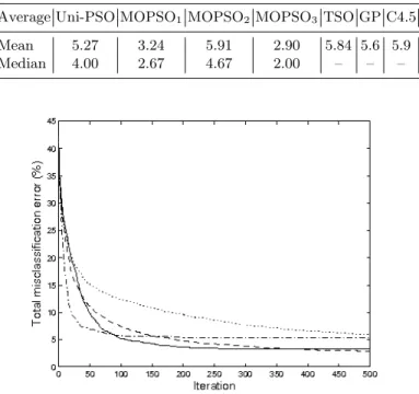
Table 1.Mean and median total misclassification error results on the Iris data set, over 100 runs after 500 iterations (see Figure 6 and 7 for plots versus iteration). Values for TSO, GP and c4.5 taken from [14].
Average Uni-PSO MOPSO1 MOPSO2 MOPSO3 TSO GP C4.5
Mean 5.27 3.24 5.91 2.90 5.84 5.6 5.9
Median 4.00 2.67 4.67 2.00 – – –
Fig. 6.Total misclassification error on Iris data versus PSO generation. Dash-dotted line denotes mean of the global individual of 100 runs using a single objective, solid line MOPSO1, dotted line MOPSO2 and dashed line MOPSO3. (For MOPSO
optimisers, global individual selected from the trade-off set based on minimising total error.)
different optimisers used. The first four are implementations of Algorithm 1, the first when minimising a single objective (uni-PSO); when minimising the individual misclassification rates7
with the dominance guide selection method (MOPSO1); minimising individual misclassification rates with the distance
guide selection method (MOPSO2); and minimising the individual
misclassi-fication rates with a (random) 50/50 use of the two different guide methods (MOPSO3). The last three columns give the mean result reported in [14] of
their single objective PSO optimiser (TSO), that of a genetic programming (GP) optimiser, and C4.5. It is encouraging to note that the optimsers intro-duced here (bar MOPSO2) outperform the results published in [14].
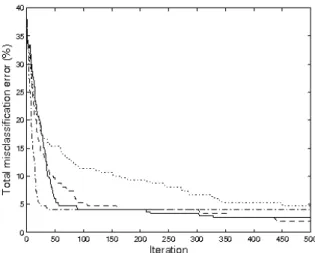
Figure 6 shows how the mean total error varies with iteration for the four PSO implementations, and Figure 7 does the same for the median. Both plots
7
As it is a 3 class problem this results in 6 different objectives, i.e. the off-diagonal elements of the confusion rate matrix.
tell the same underlying story – though it should be noted that the median is a more robust statistic. Between 10 and 60 iterations the uni-objective PSO finds significantly better solutions (with respect to total error) compared to the multi-objective optimisers. This is most likely due to its focused search. The performance of the uni-objective PSO plateaus at around 200 iterations (mean) and 50 iterations (median) – indicating it has converged. The multi-objective optimisers by comparison keep improving the total misclassification error throughout the search, with MOPSO1and MOPSO3overtaking the
uni-objective optimiser, with a significant out performance after 200-300 iterations (depending on the optimiser). MOPSO2 (with guides selected based on
dis-tance) performs less well comparatively, however it is interesting to note that it is still improving its performance throughout the search and looks set to overtake the uni-objective optimiser if run for more iterations.
The optimisers which use dominance to select their guides, exclusively or in tandem with using a distance measure, perform much better than the one which uses distance exclusively. Interestingly it is only toward the very end of the runs that the optimiser that uses a mixture overtakes that using strictly dominance. It seems likely that this is the effect of the distance selection pro-moting greater search. Toward the end of the run as the optimiser converges the inertia is very small, so if the number of global and personal best points which dominate a particle → 1 (or even are identical to the particle) the variation/search aspect may shrink prematurely. Selecting at random from a
Fig. 7.Total misclassification error on Iris data versus PSO generation. Dash-dotted line denotes median of the global individual of 100 runs using a single objective, solid line MOPSO1, dotted line MOPSO2 and dashed line MOPSO3. (For MOPSO
optimisers, global individual selected from the trade-off set based on minimising total error.)
Table 2.Properties of classification problems (sample number refers to number of complete data points in set – i.e. without missing values) [5].
Data set # classes # features # samples
Adult 2 14 48842
Breast cancer Wisconsin (original) 2 10 683
Breast cancer 2 9 277
Iris 3 4 150
Statlog (Australian credit approval) 2 14 690
Table 3.Mean and median results of uni-objective PSO and MOPSO3over 30 runs.
uni-obj MOPSO3
Data set mean median mean median
Adult 17.72 17.56 18.13 18.02
Breast cancer Wisconsin (original) 3.26 3.22 2.76 2.63
Breast cancer 21.31 21.30 21.16 21.30
Statlog (Australian credit approval) 13.53 13.62 12.68 12.75
subset of the closest global and personal bests to act as guides means the search aspect is maintained, whilst at the same time convergence is promoted by selecting 50% of the time using dominance.
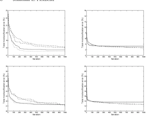
The optimisers we run on a number of other data sets taken from the UCI machine learning repository, whose details are described in Table 2. Numeri-cal results are presented in Table 3 for the uni-objective PSO and MOPSO3
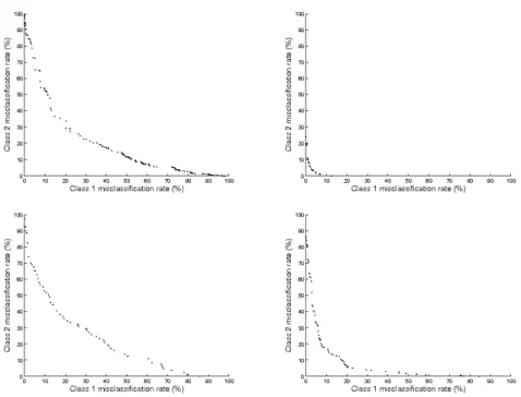
variant, running for 1000 iterations with 6 layers for these larger problems. As the results in Table 3 show, on these problems (bar the Adult data set) the multi-objective search discovers better overall (equal cost) solutions than the optimiser that is designed specifically for that objective (again in the same number of function evaluations). Not only this but at the end of the run an estimated optimal trade-offset is returned, Figure 9 shows trade-off
solutions returned by the multi-objective optimiser from a single randomly selected run on the 2-class problems. The Adult data set seems more difficult than the others for the multi-objective optimiser to push forward. Looking at Table 2, this data set has considerably more data samples than the others, meaning the possible objective combinations is also much larger. In this case MOPSO variants such as the sigma method [26] may fair better at pushing the front forward as opposed to filling it out.
The Iris problem having 6 objectives is less easy to visualise in this for-mat, so an alternative representation is provided in Figure 10, providing a histogram of the the distances of points on the trade-off front from the ran-dom allocation simplex [15, 16]. The ranran-dom allocation simplex is the plane in misclassification rate space which denotes classifiers which assign classes to data points at random (with some probability). For the 3-class (6
objec-Fig. 8. Average total misclassification error over 30 runs. Solid line, mean uni-objective PSO, dotted line median uni-uni-objective PSO, dashed line mean MOPSO3,
dash-dotted line median MOPSO3. Top right plot Adult dataset, top right Breast
cancer Wisconsin (original) data set, bottom left Breast cancer data set, bottom right Statlog (Australian credit approval) data set.
tive) problem, the optimal point at the origin is an absolute distance of 2 (number of classes-1) from the random allocation simplex. In keeping with the minimisation representation, points between the origin and random allo-cation simplex are given negative distances and points behind (worse than) the random allocation simplex are given positive distances. As is clear, the vast majority of points represent classifiers that perform better than random, with a number a great distance in front of the random allocation simplex.
7 Summary
This chapter has covered the optimisation of decision trees, both with single and multiple objectives, utilising the representation originally introduced in [14] for single objective optimisation, and drawing on the extensive work in the literature on applying PSO to multi-objective problems. Key results not only include the success in general of applying multi-objective PSO to decision tree classification problems, able to find a set of decision trees which trade-off
Fig. 9. Example trade-off fronts. Top right plot Adult data set, top right Breast cancer Wisconsin (original) data set, bottom left Breast cancer data set, bottom right Statlog (Australian credit approval) data set.
−2 −1.5 −1 −0.5 0 0.5 0 0.5 1 1.5 2 2.5 3 3.5 4
Distance from random allocation simplex
Number of classifiers
Fig. 10.Distance of global best points from the random allocation simplex, taken from a single run of MOPSO3on the Iris data set. The distance value of -2 relates to
the optimal (typically not achievable) origin. A point with a distance value greater than zero is worse than random.
the different misclassification error rates, but that it also tends to find better single objective solutions compared to uni-objective PSO.
The multi-objective PSO experienced slower convergence and worse per-formance with the larger Adult dataset. It would be useful to investigate this
further in future to see if there actually is a correlation between size and com-parative performance. This may be a result of the fact that as the data set size increases theresolutionin objective space also increases, making the potential number of points on any front increase and thereby impede convergence. Data subsampling or algorithms with greater convergence pressure make be more appropriate for these types of problem.
The multi-objective PSO variant with an equal mix of dominance based guide selection and distance based guide selection performed best of the three variants compared, with the assessment that this was due to its mixing of convergence properties and search properties. A similar effect may well be found by having a different weighting between the guide selection (as the dominance approach does tend to converge faster, and not plateau like the uni-objective variant), or alternatively using a turbulence (mutation) term (see e.g. [21]).
A final point of note is the size of representation (and therefore size of the search space) is influenced by the maximum number of layers in the decision tree, the number of features and the number of classes. There is a potential if these are high for the search landscape to become excessive, with large flat (uninformative) sections, even with respect to multiple objectives. As such investigation into smaller representations for continuous optimisers, or for discrete PSO, would be worth investigating.
References
1. Bishop, C. (2006)Pattern Recognition and Machine Learning. Information Sci-ence and Statistics, Springer.
2. Duda, R. and Hart, P. (2001)Pattern Classification and Scene Analysis. Wiley, 2 edn.
3. Everson, R. and Fieldsend, J. (2006) Multi-objective optimisation of safety re-lated systems: An application to short term conflict alert. IEEE Transactions
on Evolutionary Computation,10, 187–198.
4. Schetinin, V., Fieldsend, J., Partridge, D., Coats, T., Krzanowski, W., Everson, R., Bailey, T., and Hernandez, A. (2007) Confident interpretation of bayesian decision tree ensembles for clinical applications.EEE Transactions on
Informa-tion Technology in Biomedicine,11, 312–319.
5. Asuncion, A. and Newman, D. (2007), UCI machine learning repository. 6. Ripley, B. (1994) Neural networks and related methods for classification (with
discussion).Journal of the Royal Statistical Society Series B,56, 409–456. 7. Brieman, L., Friedman, J., Olshen, R., and Stone, C. (1984)Classification and
Regression Trees. Chapman & Hall/CRC.
8. Quinlan, J. (1986) Induction of decision trees.Machine Learning,1, 86–106. 9. Quinlan, J. (1993) C4.5 Programs for Machine Learning. Machine learning,
Morgan Kaufmann.
10. Kennedy, J. and Eberhart, R. (1995) Particle swarm optimization. IEEE
In-ternational Conference on Neural Networks, Perth, Australia, pp. 1942–1948,
11. Kennedy, J. and Eberhart, R. (1997) A discrete binary version of the particle swarm algorithm. Proceedings of the IEEE Conference on Systems, Man and
Cybernetics, pp. 4104–4109, IEEE Press.
12. Kim, D. (2006) Minimizing structural risk on decision tree classification. Jin, Y. (ed.),Multi-Objective Machine Learning, vol. 16 ofStudies in Computational
Intelligence, pp. 241–260, Springer.
13. Denison, D., Holmes, C., Mallick, B., and Smith, A. (2002) Bayesian Methods
for Nonlinear Classification and Regression. Probability and Statistics, Wiley.
14. Veenhuis, C., K¨oppen, M., Kr¨uger, J., and Nickolay, B. (2005) Tree swarm optimization: An approach to pso-based tree discovery.2005 IEEE Congress on
Evolutionary Computation, vol. 2, pp. 1238–1245.
15. Everson, R. and Fieldsend, J. (2006) Multi-class roc analysis from a multi-objective optimisation perspective.Pattern Recognition Letters,27, 918–927. 16. Everson, R. and Fieldsend, J. (2006) Multi-objective optimisation for receiver
operating characteristic analysis. Jin, Y. (ed.),Multi-Objective Machine Learn-ing, vol. 16 ofStudies in Computational Intelligence, pp. 531–556, Springer. 17. Fieldsend, J. (2004) Multi-objective particle swarm optimisation methods. Tech.
Rep. 419, Department of Computer Science, University of Exeter.
18. Coello Coello, C., Pulido, G., and Lechuga, M. (2004) Handling multiple ob-jectives with particle swarm optimization. IEEE Transactions on Evolutionary
Computation,8, 256–279.
19. Alvarez-Benitez, J., Everson, R., and Fieldsend, J. (2005) A mopso algorithm based exclusively on pareto dominance concepts.The Third International
Con-ference on Evolutionary Mutli-Criterion Optimization, pp. 459–473.
20. Fieldsend, J., Everson, R., and Singh, S. (2003) Using unconstrained elite archives for multi-objective optimization. IEEE Transactions on Evolutionary
Computation,7, 305–323.
21. Fieldsend, J. and S.Singh (2002) A multi-objective algorithm based upon par-ticle swarm optimisation, an efficient data structure and turbulence. 2002 UK
Workshop on Computational Intelligence (UKCI’02), Birmingham, UK, pp. 37–
44.
22. Fieldsend, J. and Singh, S. (2005) Pareto evolutionary neural networks.IEEE
Transactions on Neural Networks,16, 338–354.
23. Knowles, J., Watson, R., and Corne, D. (2001) Reducing local optima in single-objective problems by multi-objectivization. Zitzler, E., Deb, K., Thiele, L., C.Coello, C., and Corne, D. (eds.), First International Conference on
Evolu-tionary Multi-Criterion Optimization, Lecture Notes in Computer Science, pp.
269–283, no. 1993.
24. Jensen, M. (2003) Guiding single-objective optimization using multiobjective methods. Cagnoni, S., et al. (eds.), Applications of Evolutionary Computing: EvoWorkshops 2003: EvoBIO, EvoCOP, EvoIASP, EvoMUSART, EvoROB,
and EvoSTIM, Lecture Notes in Computer Science, pp. 268–276, no. 2611.
25. Abbass, H. and Deb, K. (2003) Searching under multi-evolutionary pressures. Springer-Verlag (ed.),Proceedings of the 2003 Evolutionary Multiobjective
Op-timization Conference (EMO03), pp. 391–404.
26. Mostaghim, S. and Teich, J. (2003) Strategies for finding good local guides in multi-objective particle swarm optimization (mopso).IEEE 2003 Swarm