Master's degree in Automatic Control and Robotics
Optimization of common
computer vision algorithms
Beating OpenCV Face Detector MEMORY
Author: Albert Pumarola Peris Director/s: Cecilio Angulo Bahón
School: School of Industrial Engineering of Barcelona Call: June 2016 2 01 6 M ast er 's d eg re e in A u to m a tic C on tr ol a nd R ob otics A lbe rt P uma rol
Escola Tècnica Superior
In this Master Thesis one of the most common problems related to face detection is presented: fast and accurate unconstrained face detection. To deal with this problem a new general learning method is presented.
The proposed method introduces a set of upgrades and modifications on key concepts and ideas of Decision Trees, AdaBoost and Soft Cascade learning techniques. Firstly, a new variation of Decision Trees with quadratic thresholds able to maximize the margin distance between classes is introduced. Considering a training set independent of face orientation and viewpoints information, the proposed algorithm is able to learn a com-bination of features to cluster faces under unconstrained face position and orientation. Next, a new definition of the Soft Cascade thresholds training principles is provided. Hence, this modification leads to a better formulation of the loss function associated to the AdaBoost algorithm.
The trained face detector has been tested over the Face Detection Data Set and Bench-mark (FDDB) and compared against the current state of the art classifiers. The obtained results show that the proposed face detector (i) is able to detect faces with unconstrained position, and (ii) it works faster than the current state of the art methods.
Abstract i
List of Figures iv
List of Tables v
Abbreviations vii
Mathematical notation viii
1 Introduction 1
1.1 Information, context and project description. . . 1
1.2 Scope . . . 3
1.3 Objectives . . . 3
1.4 Resources . . . 4
2 State of the art 6 3 Theoretical background 8 3.1 AdaBoost . . . 8
3.2 Weak classifiers. Decision Trees . . . 10
3.3 Soft Cascade . . . 13
3.4 Support Vector Machines . . . 15
4 Proposed learning method 18 4.1 Weak classifiers. Decision Tree . . . 18
4.2 Soft Cascade . . . 23
4.3 AdaBoost . . . 25
4.4 Strong Classifier as a Final Filter . . . 27
4.5 Modern and Highly Optimized Code with SIMD Instructions . . . 28
5 Features 30 5.1 Haar-like features . . . 30
5.2 Normalized Pixel Difference . . . 32
5.3 Histogram of Oriented Gradients . . . 33
6 Temporary planning 35 6.1 Tasks identification . . . 35
6.1.1 State of the art and learning . . . 35
6.1.2 Debugging dataset generation . . . 35
6.1.3 Learning classifier . . . 36
6.1.4 Features . . . 36
6.1.5 Learning algorithm . . . 36
6.1.6 Final dataset generation . . . 36
6.1.7 Classifier training and validation . . . 36
6.1.8 Classifier implementation optimization . . . 37
6.1.9 Final documentation . . . 37
6.2 Time estimation . . . 37
6.3 Initial planing . . . 38
6.4 Final planning . . . 38
7 Experimentation and results 41 7.1 Proof of concept - basic tests . . . 42
7.2 Learned cascade decision trees . . . 43
7.3 Evolution of the training samples scores and thresholds . . . 45
7.4 Evolution of the training samples quantity . . . 45
7.5 Evolution of the testing samples scores . . . 46
7.6 Rejection evolution of the testing samples in the cascade . . . 47
7.7 Non-maximum suppression as afilter . . . 49
7.8 Real time . . . 49
7.9 Benchmark . . . 51
8 Sustainability and social commitment 55 8.1 Economical impact . . . 55
8.2 Social impact . . . 56
8.3 Environmental impact . . . 56
9 Conclusions and future work 58 10 Costs 61 10.1 Hardware costs . . . 61
10.2 Software costs . . . 62
10.3 Human resource costs . . . 62
10.4 Overhead costs . . . 64
10.5 Total costs . . . 64
10.6 Economic viability . . . 65
3.1 Dummy example of AdaBoost. . . 9
3.2 Example of a Decision Tree. . . 11
3.3 Binary entropy function . . . 12
3.4 Cascade structure. . . 13
3.5 Cascade score trace. . . 14
3.6 A Support Vector Machine. . . 15
4.1 Three possible NPD cases to be represented. . . 20
4.2 Approximate maximal margin. . . 23
4.3 Problem with traditional AdaBoost loss function. . . 27
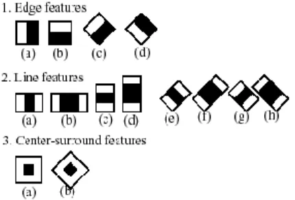
5.1 Haar-like kernels feature description. . . 31
5.2 Normalized pixel difference representation. . . 32
6.1 Gannt diagram initial planning . . . 38
6.2 Gannt diagramfinal planning.. . . 39
7.1 Two linearly separable basic test with two featuref ∈[0,255]. The radius of each sample represents its weight. . . 42
7.2 First nonliear basic test with two featuref ∈[0,255]. The radius of each sample represents its weight. . . 42
7.3 Second nonliear basic test with two feature f ∈ [0,255]. The radius of each sample represents its weight.. . . 43
7.4 Learned cascade decision trees. . . 44
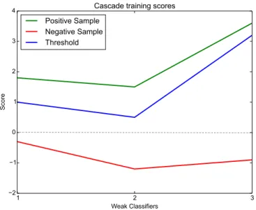
7.5 Evolution of the training samples scores and thresholds. . . 45
7.6 Evolution of the training samples quantity. . . 46
7.7 Evolution of the testing samples scores. . . 48
7.8 Evolution of the testing samples live. . . 49
7.9 Real time video frame showing non-maximum suppression. Blue bounding boxes are all the face detections, the green one is thefinal detection. . . . 49
7.10 ROC curves of the FDDB benchmark. . . 52
7.11 Correctly classified samples of the FDDB benchmark. . . 54
6.1 Time estimation table of the initial planning. . . 37
6.2 Time estimation table final planning.. . . 40
7.1 Confusion matrix. . . 47
7.2 Unconstrained face detection speed comparison. . . 50
7.3 Speed of our method vs the once currently being used. . . 50
7.4 Space and memory of our method vs the once currently being used. . . . 50
10.1 Hardware Costs Table. . . 61
10.2 Software Costs Table. . . 62
10.3 Human resources costs table 1/2. . . 63
10.4 Human resources costs table 2/2. . . 64
10.5 Overhead costs table.. . . 64
1 Soft Cascade rejection function . . . 14 2 Integral Image. . . 31
CMU CarnegieMellonUniversity
RAM Random AccessMemory
GPU GraphicsProcessor Unit
CPU CentralProcessing Unit
II Integral Image
NPD NormalizedPixel Difference
HOG Histogram of OrientedGradients
I Image
H(x) Strong Classifier h(x) Weak Classifier
f Feature
ws Weight of a sample s
αt Weight of a Cascade Weak Classifiers ht(x)
θt Threshold of a Cascade Weak Classifiersht(x)
Sj Node j of a Decision Tree
SL
j,SjR Left and right sons of a Decision Tree node Sj
Introduction
1.1
Information, context and project description
It is said that the face is one of the most powerful channels of non-verbal communication. Data extracted from a person’s facial behaviour can be used as a predictor of his/her internal states, social behaviour, biometrics and psychopathology. In other words, just by analyzing a person’s facial behaviour we could estimate if that person suffers from depression, the level of interest of an audience attending a talk, car drivers fatigued, even detecting security issues. These are just some of the applications of the face analysisfield, but its possibilities are limitless. Face analysis pipelines are really complex an diverse, but they all have one common component, aface detection step. This step is critical as no analysis can be performed without first detecting the person face. Hence, the main goal of this project is to develop a fast, accurate and unconstrained face detector. Face detection is a well studied problem in the Computer Vision research area. Modern face detectors can easily detect frontal faces near to the camera and it is a well solved problem. Current research focuses on detection of faces in unconstrained positions. In this case, there are two main difficulties: large visual variations of the same face due to illumination, occlusions, expression variations and image resolution; and the huge search space of possible face positions and sizes for a given image. Current state of the art algorithms obtain very good detection results, but with a very high computational complexity.
The new proposed learning method introduces a set of upgrades and modifications of the key concepts and ideas of Decision Trees, AdaBoost and Soft Cascade. First, a new variation of Decision Trees is presented. Upgraded with quadratic thresholds and able of maximizing the margin distance it is capable of learning the optimal combination of features to cluster faces under unconstrained face position and orientation. Moreover, the proposed solution does not require face orientation and viewpoints training labels. It is capable of automatically clustering the different viewpoints at their lower levels. Hence, the learned face detector is more robust to unconstrained faces than the state-of-the-art methods based on learning one model for each of the possible views, and then, for a given sample, trying to guess which ones to run.
Second, a new definition of the Soft Cascade thresholds learning method is proposed. Instead of first training the cascade and then calibrating the thresholds, it is proposed to learn them during the training stage. Furthermore, instead of learning them with the current na¨ıve based approach used in the current state of the art Soft Cascade, thresholds are learnt using a data-based method relying on support vector machines. Third, by joining the learning and calibration stages of the Soft Cascade learning, it is opened the possibility to define a better formulation of the AdaBoost loss function. The trained face detector has been tested over the new Face Detection Data Set and Benchmark (FDDB) and proved to achieve state-of-the-art performance and beat in terms of memory, speed and accuracy the Viola-Jones method and most of the current state-of-the-art methods.
The associated research work leading to this Master Thesis has been developed at the Carnegie Mellon Robotics Institute, in the Human Sensing Lab. The mission in this research laboratory is to develop advanced computational tools to model and understand human behavior from sensory data. Their main research topics are human sensing, component analysis and face analysis.
The implemented face detector will be used as the face detection module of their face analysis pipeline. It represents a high honor and responsibility to design and imple-ment the face detection module because this laboratory is considered to be one of the best ones in face analysis research. They are currently using the Viola-Jones OpenCV implementation. Thus, the main goal is to beat this detector.
1.2
Scope
As a main goal in this Master Thesis, a new learning method for face detection will be designed and implemented from scratch, without the use of any particular library, but image data manipulation and Support Vector Machines. Its main purpose will be to detect faces which will after be analyzed to extract behavioral states of a person in real time. Neither data extraction nor analysis can be performed if the face is not well detected, hence the detector module must work in real time with high detection accuracy. It is also desired that the detector works with unconstrained positions. It is out of the scope of this project to detect small-blurry faces or faces with high level of occlusion because even if detected, no good posterior analysis could be performed. Work in this thesis is more than a theoretical research, but a real world product re-lease project. The designed detector will work in a constrained laboratory environment, but also must be robust to real world problems as well as memory and computation complexity. The implemented detection algorithm will not only run on computers, but also on devices with less computational power such as smartphones and tablets. As a consequence, its computational complexity must be very low, and cannot rely on a GPU for better reason. Its memory complexity must also be low because cellular users are not prompted to install apps asking for high memory resources. For the scope of this project, it is also supposed that the device has at least 1GB of RAM, a dual-core processor and a camera with a minimum resolution of 500x480 pixels.
1.3
Objectives
The main objective of this project is to implement a face detector working on popular cellulars with the following features:
• Beat the current face detector module used in the laboratory pipeline, the Viola-Jones OpenCV implementation.
• All the designed training algorithms and features must be implemented from zero (except the Support Vector Machine algorithm).
• Low computational complexity: the module should run at a minimum speed of 100 Hz on a dual-core processor, in GPU-denied devices.
• Low memory complexity: it should be able to run with a maximum memory consumption of 500 MB and with a model lower that 15 MB.
• State-of-the-art accuracy for fast algorithms should be obtained.
• Detect faces with unconstrained position in cluttered environments.
• Highly modular: It should be easily adapted to new features and classifiers.
• Modern code: all algorithms and features must be implemented with highly effi -cient, CPU optimized modern code.
• Transparent: develop a set of scripts which can display and plot the behaviour of the detector and the learning process to make them as much transparent as possible.
Personal objectives:
• Learn
• Learn
• Learn... not only theoretical knowledge but also the way of working and un-derstanding the passion and almost an obsession of Carnegie Mellon University researchers.
• Enjoy the experience of being on one of the best computer vision university and research groups.
1.4
Resources
Hardware
• Server where the proposed training algorithm is executed. 20 cores Xeon E7 v2/Xeon E5 v2/Core i7 DMI2, 180 GB of memory, no graphic cards.
• Sony Vaio computer where the learned model is tested in real time.
Software
• Ubuntu 12.04
• Vim text edtior.
• ShareLaTeX, LATEXonline text editor.
• BitBucket, a github web-based hosting service.
• Mendeley, a PDF manager and reader.
Humans The author of this project and the members of the Human Sensing Lab
experts in the field of computer vision. These experts will bring feedback during the development of the project.
State of the art
Face detection is a deeply studied problem and a lot of different approaches and methods have been developed. The most cited work in this field is the famous Viola and Jones paper [1] which introduced in 2013 the concepts of Integral Image based Haar features, AdaBoost based learning model and the combination of the classifiers in a Cascade structure. Since then, a lot of new approaches mainly focused on using different types of features and classifiers have been proposed. Currently we can cluster all methods in ei-ther, traditional or modern approaches. Traditional approaches are based on traditional classifiers such as Support Vector Machines (SVM) [2], AdaBoost with Cascade [1] and random Decision Trees [3]. In the other hand, modern approaches are based on using highly complex non-linear models generated with Deep Learning [4–6] or by using a 3D model of the face [7].
Main differences between both approaches are the size of the training data and time needed to train, the computational and memory complexity, and accuracy. Traditional approaches require much less number of samples and time to train, and they also have a much lower computational and memory complexity, making them much faster than modern approaches. However, modern approaches lead to higher accuracy. They claim to obtain even a higher accuracy than a human. Highly difficult benchmarks like FDDB [8] show how modern approaches have an accuracy of almost 90% vs 50% of traditional approaches. However, this high accuracy leads to a high computational complexity (15s for a full-HD image) v’s 10ms in traditional approaches. There are multiple works which
try to merge these two approaches, trying to get the best of both approaches. A common way is by having a Cascade of Convolutional Neural Networks (CNNs) [6,9].
This project will focus on traditional approaches because of the real time constraint. Most traditional face detection methods are appearance based.Many different features has been proposed such as Haar [1], Local Binary Pattern (LBP) [10], Histogram of Gradients (HoG) [11], SURF [12], Local Binary Pattern histogram [13] and Normalized Pixel Difference (NPD) [14]. Detectors with manually defined features are usually faster in speed but more simple [15]. The most famous ones are based on Haar kernels which are the most common used features for frontal face detection. Texture based methods like LBP have been proven to be robust in front of monotonic light changes. HoG is able to better generalize non-face images, but has a higher computational cost. SURF features improve face detection performance by due to its high dimensionality it critically slows down the training process. Comparison of pixel intensity features [14,16,17] does not contain as much information as conventional features, but they are much faster as they do not need to process anything by using a look-up-table.
Not only different features have been introduced in the literature, but also modifications in the AdaBoost algorithm, like Vector Boost [18] and MBHBoost [19], as well as the election of the boosting weak classifiers. Multiple studies [14, 20] have demonstrated that using Decision Trees (CART) as the boost weak classifier tends to give much better results than just a simple Stump.
All state-of-the-art traditional methods have troubles when trying to detect multiview faces. Most common approaches consist of training a set of cascade detectors for each possible view, such as Parallel Cascade [21] and Pyramid architecture [22]. To avoid having to execute all models for each one of the evaluated regions of interest (ROI) they propose a previous step in which an approximation of the face orientation is estimated and only the classifiers near to that configuration are evaluated. Training of multiple classifiers for all the possible face position configurations increase the computational and memory complexity as well as the amount of labeling required. Moreover, a bad estima-tion of the face posiestima-tion would lead to face not to being detected. It is proposed in [14] a method based on Deep Quadratic Trees to automatically learn a general unconstrained face position model without the need of a labeling stage.
Theoretical background
The implemented face detector is based in a Soft Cascade of weak classifiers trained with Adaboost. In this chapter all the theoretical background related to the framework is presented.
3.1
AdaBoost
Boosting is an approach to machine learning based on the idea of creating a highly accurate classifier by combining many simple and easy to find rules / subclassifiers. Freund and Schapire [23] proposed AdaBoost, the first practical boosting algorithm. The idea is to ensemble a set of T weighted really simple classifiers with an error rate just below random, called weak classifiers, to create a higher order classifier named strong classifier. Boosting methods are expressed as:
H(x) =
T
�
t=1
sign(αtht(x)) (3.1)
whereH(x) is the strong classifier which is composed byT weak classifiers ht(x),
ht(x) =
+1, ifx classified as a positive sample
−1, ifx classified as a negative sample
(3.2)
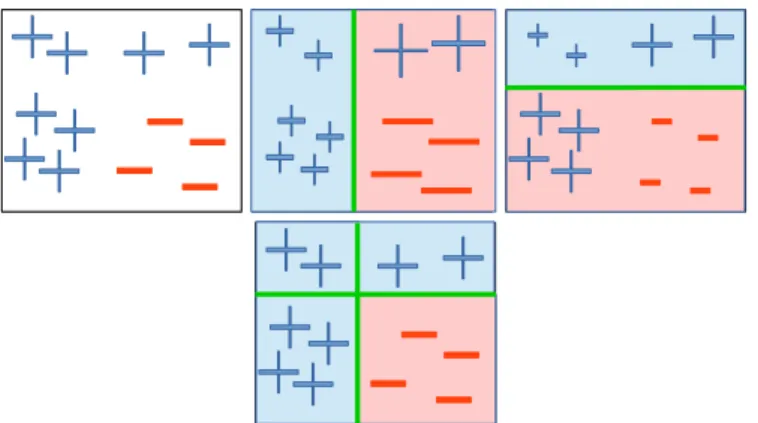
Figure 3.1: Dummy example of AdaBoost.
A dummy example can be seen at Figure 3.1, where the size of the samples represent their weights and the green lines the weak classifiers. The final classifier (bottom line) is a weighted combination of booth learned weak classifiers (top line).
AdaBoost proposes to learn iteratively the weak classifiers and their corresponding weights. At a given step t, the weak classifier ht(x) with lowest error rate, in a
con-strained time window, is found; then, you find its corresponding weight αt; finally,
samples weight is updated increasing those which were misclassified in order to empha-size them when learning the next weak classifierht+1(x). The algorithm is stopped when
either, the desired classification rate is reached or no more weak classifier can be learned because the defined maximum number has been attained.
At thefirst step, all samples have the same importance, so they all have the same weight:
w1s = 1
n (3.3)
wheresis the index of a sample andnthe number of samples. Hence, the error rate for a particular step can be computed as the sum of the weights for the samples that were misclassified by the new learned weak classifier:
et= N
�
i=1
wi|ht(xi)−yi|, whereN is the number of samples (3.4)
Once computed the error et of the current weak classifier ht(x), Freund and Schapire
bound, and eventually go to zero: αt=− 1 2log � et 1−et � (3.5)
If we analyze the formula for αt, it can be easily seen that the weight given to a weak
classifier is the inverse of the classification error. In other words, higher classification rate has a weak classifier, higher weight is assigned to. Weak classifiers with higher classification rate will have a higher contribution on the final strong classifiers
The last reaming step is to update the weights assigned to samples based on the new weak classifier ht(x). To do so there are two common approaches. The first one is to
update the weights based on the classification rate of the new weak classifier,
wst+1 = wt s Nt e−αt, if s correctly classified wst Nt e+αt, if s misclassified (3.6)
The other approach is to understand Boost as a gradient descent method where the loss function to be minimized is �ie−yiαtht(xi). The idea is to maximize the score of the
positives samples and minimize the score of the negatives samples. With this approach the weights are updated as,
wts=wts−1e−ysαtht(xs) (3.7)
As a summary, at each iteration, chooseht(x) which minimizeset=�Ni=1wi|ht(xi−yi)|.
Then, set the weight of ht(x) to beαt=−12log
� et 1−et � and update Ht(x) =Ht−1(x) + αtht(x).
3.2
Weak classi
fi
ers. Decision Trees
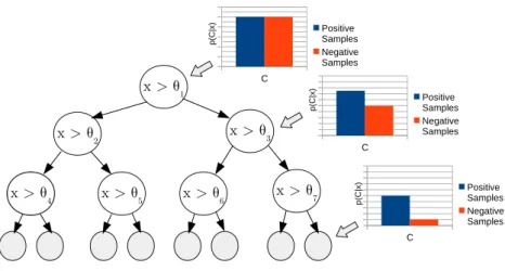
Decision Trees [24] classifiers are tree-like graph models of decisions where nodes rep-resent features and branches reprep-resent splits of the data based on the feature result. The most common weak classifiers used in face detection with AdaBoost Cascade are Decision Stumps. Decision Stumps are 1-rule decision models which predict a classifi ca-tion result based on one single feature. They can be seen as 1-level Decision Trees (see Figure3.2).
x > θ1 x > θ2 x > θ3 x > θ 4 x > θ5 x > θ6 x > θ7 x > θ4 C Positive Samples Negative Samples p(C|x) C Positive Samples Negative Samples C Positive Samples Negative Samples p(C|x) p(C|x)
Figure 3.2: Example of a Decision Tree.
A given sample to be classified is inserted to the Decision Tree from the root node where it is tested with one feature. Based on the evaluation result, the sample goes down through the left or right branch. The node connected to the followed branch is then evaluated and the sample is again redirected left or right. This process is repeated until reaching a leaf with and assigned label to it. The sample is label with the same label as the one assigned to the leaf where it has fallen.
The construction of the tree consist on partitioning the training data in each leaf in a way that the classification error at each leave decreases. The feature that best splits the samples into the purest possible children nodes is chosen. Measuring how pure a subset of samples is the same as measuring the amount of information that would be needed to correctly label a given sample in that subset. This can be calculated as the difference of probabilities of the labels in the subset. However, the common approach to decide the feature to assign to a node is by calculating the opposite. Instead of calculate the purity, the impurity of the subsets is measured with the entropy. The entropy of a random subset is measured as:
H =−�
y∈Y
P(y) logP(y) (3.8)
where Y are all the possible class labels. The entropy for a binary set of samples containingp positives samples and nnegative ones is:
H � p p+n, n p+n � =− p p+nlog p p+n− n p+nlog n p+n (3.9)
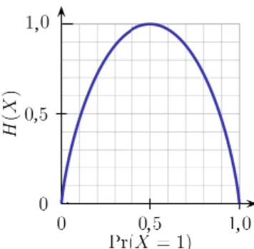
Figure 3.3: Binary entropy function
when there is the same probability of being of any of booth classes (p(X =a) = 0.5 or p(X =b) = 0.5). Opposite to that, its minimum value 0 is reached when the probability of being of one class is 1 (p(X =a) = 1 or p(X=a) = 0). Therefore, to minimize the classification rate at each level of the tree it is necessary that its reducing uncertainty of the prediction at each tree levels keeps decreasing. In other words, the entropy comparison between the parent node and its sons gives a measure of the information gained by doing the split using that particular feature. This can be expressed as:
Ij =H(Sj)− � i∈{L,R} |Si j| |Sj| H�Sji� (3.10)
where SjL, SjR are the two sons of node Sj. At each node of the tree, the feature with
highest information gain is selected. This process is applied recursively to its sons until one of the stop criterion is satisfied. There are multiple stop criterion such us reaching the maximum level of the tree or reaching a sub-state with null entropy.
To avoid overfeeding, once the tree has been constructed a trim step is performed. In this step, the nodes that do not improve the information gained or its contribution is very low are removed.
At each leaf of the tree there are set of p positives samples and n negatives samples which can be represented with a histogram (see Figure3.2). Hence, the probability of a new sample that has fallen into that leaf of being positive is P(x =pos) = p+pn and being negativeP(x=neg) = p+nn.
𝛼1h1(x) T 𝛼2h2(x) T 𝛼3h3(x) T 𝛼nhn(x) T F F F F T ... Reject Post Processing Sample
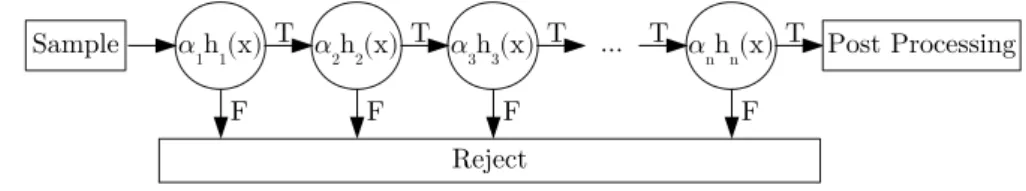
Figure 3.4: Cascade structure.
3.3
Soft Cascade
One of the principal problems when training classifiers is the trade-offbetween accuracy and speed. This problem becomes even bigger when applying boost techniques. Eval-uating all the weak classifiers for a given sample produces, normally, higher results of precision but at a higher computational cost. A common way to solve this problem is by applying a cascade structure.
Cascade structures (see Figure3.4) decomposes a strong classifier into a linear sequence of weak classifiers. For a given stage of the cascade, all the samples classified as positive for the current weak classifier are sent to the next stage. Samples classified as negatives are rejected. Only the samples which pass all the stages of the cascade are finally classified as positive.
The intuition behind this strategy is that there is a significant statistical dependency among the features. Hence, a lot of samples can clearly be rejected by the first weak classifiers without the need of evaluating all the rest.
There are two main problems with cascade structures. First, information obtained in one of the stages of the cascade is discarded as it passes to the next stage. Second, all true positive samples must be classified as positive by all the weak classifiers to be classified as positive.
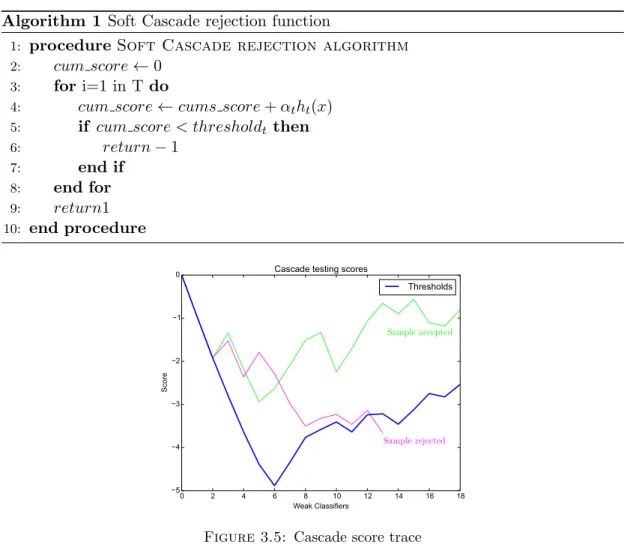
These two problems are solved by Soft Cascade. Instead of having a sequence of binary stages, it proposes to have a sequence of stages each giving a score on how well a given sample passed that stage. At each stage of the cascade the cumulative sum of all the previous stages plus the current one is evaluated. If this value is higher than a training threshold the sample is sent to the next stage, otherwise it is discarded. The pseudo code of this rejection function is shown in Algorithm 1.
Algorithm 1 Soft Cascade rejection function
1: procedureSoft Cascade rejection algorithm
2: cum score←0
3: fori=1 in T do
4: cum score←cums score+αtht(x)
5: if cum score < thresholdt then
6: return−1 7: end if 8: end for 9: return1 10: end procedure Sample rejected Sample accepted
Figure 3.5: Cascade score trace
In this way samples are not prematurely rejected. Samples which did good in several weak classifiers but failed in one are not discarded because they accumulate a score high enough to keep them alive. Moreover, each weak classifier has a weight α assigned to it. Hence, samples with high score in the important classifiers are more likely to be finally classified as positive samples. A score trace is presented in Figure3.5. As it can be seen, scores that at some point are lower than the rejection trace are rejected and automatically classified as negatives. Those that are not rejected by the cascade are considered positive.
Some modifications of the original AdaBoost algorithm must be performed to train the cascade. Now, training samples can be rejected by a training rejection function defined as: t � j=1 αjhj(x)≥ 1 2 t � j=1 αj (3.11)
At a given stage t only samples with a cumulative score higher or equal than half of the sum of previous classifiers weightsαj are selected. By eliminating training samples,
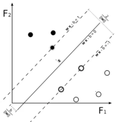
Figure 3.6: A Support Vector Machine.
more precise and specialized weak classifiers are learned as the cascade advances as they are only required to learn the subset of samples that the previous classifiers were not able to reject.
When deleting training samples, at each stage of the cascade classifiers have less training samples to manage. To solve this issue, bootstrap is introduced. Each time a new weak classifier must be trainedK new negative samples are introduced. These negative samples must satisfy the condition that they are miss-classified by the current strong classifier H(x). The number of samples K to be added is critic. If K is too large, AdaBoost will not be able to catch up and the error rate over the negative training set will be high. If K is too small, to achieve a good false positive to many weak classifiers would be required.
The last missing parameter to tune is how to decide the thresholds of the rejection function. To do so, a tuning stage is performed after all the cascade has been learned using new samples not previously seen by the classifier. Firstly, a maximum of positive samples that can be rejected at each stage is set. Then, for each stage all the new samples are evaluated and the threshold is set to be the maximum possible value which satisfy the number of positive samples to be rejected.
3.4
Support Vector Machines
Support vector machines [25] are one of the most popular supervised learning models for classification and regression analysis. SVM tries to find the optimal maximum margin hyperplane that best separate the sample classes (see Figure3.6).
The hyperplane can be we written as the set of points xwhich satisfy the condition:
w·x+b= 0 (3.12)
where w is a vector perpendicular to the hyperplane. Therefore, given a sample ex-pressed as the vectorxit can be determined in which side of the hyperplane it is located by projectingx tow. The decision rule is expressed as:
� y = +1, ifw·x+b≥0 −1, ifw·x+b <0 (3.13)
The maximum-margin hyperplane is situated between the two parallel hyperplanes that separates the two classes (as it can be seen infigure 3.6). This two hyperplanes can be
expressed as: w·x++b≥+1 w·x−+b≥ −1 (3.14)
Introducing the term yi
� y= +1, ifiis a positive sample −1, ifiis a positive sample (3.15) it results in: w·x++b≥+1⇒yi(w·x++b)−1≥0 w·x−+b≤ −1⇒yi(w·x−+b)−1≥0 (3.16)
Now booth equations have the same structure. Hyperplanes fall into the support vectors, taht is those with constraint equal to zero,
yi(w·xi+b)−1 = 0 (3.17)
The distanced to be maximized can be represented as
d= (x+−x−)·
w
wherex+,x− are two support vectors and wa vector perpendicular to the hyperplane. Then, by using Equation3.15, Equation 3.18can be transformed as,
(1−b+ 1 +b)· w
�w� =
2
�w� (3.19)
The SVM must achieve:
min1 2
�
�w2�� (3.20)
To minimize Equation3.20, Lagrange multipliers can be applied and obtain that:
maxL= 1 2 � αi− 1 2 � i � j αiαjyiyjxi·xj (3.21)
It is important to notice that becauseLdefines a convex space SVM will never fall into local maxima, but a global one exist. This formulation works for linearly separable data. If data is not linearly separable, samples are transformed into another space which there can be separable.
Our samples are not linearly separable hence, a kernel transformation could be applied. However, only linear SVMs will be used in this woirk to be able to achieve the real time constraint.
Proposed learning method
In this Chapter modifications for a Cascade of Weak Classifiers with AdaBoost are proposed, which will improve the classification results in the literature as well as to speed up the training and classification computational time.
4.1
Weak classi
fi
ers. Decision Tree
As previously seen, most face detectors use boosted stumps as weak classifiers. They present two main limitations. First, they are not capable of representing interaction between different feature dimensions. Second, the simple one-threshold splitting strategy can express a low amount of information. This section introduces a set of proposed modifications to solves this problems.
Depth of the Decison Trees
Most approaches in the literature achieve multiple-view detection by training one classi-fier for each view. Notice that a window with a face in it will only be correctly classified as a face if the classifier corresponding to the face view is used. To classify a given window there are three possible strategies: use all the classifiers, use only one or use a subset. Thus, the main problem with this approach is the trade-offbetween speed and classification rate during testing. In the literature, a pre-classification stage is added to chose which subset of classifiers should be used for each given windows. The problem
with this strategy is that if the pre-classification stage fails to return a set containing the correct classifier the windows will be miss-classified.
Our proposed method does not need to have one classifier for each view, instead only one classifier for all the views is trained thanks to the tree structure. A tree structure allows to organize the evaluated windows as they go down the tree. Then, by increasing the depth of the tree its complexity also increases and, as a consequence, its able to better cluster the evaluated windows in its leafs. In the literature for face detection classifiers the common used height is only 1 (Decision Stumps). Instead, in this project the proposed Decision Trees are of height 5, that is Decision Trees having 5 levels of depth. This value has been tuned using cross-validation experiments. In this way we can express much more complex relations between features which allow a better the views than Decision Stumps.
Notice that the cross-validated height of the tree is much higher than the one used in the literature for face detection which are only of height 1 (decision stumps). Having Decision Trees with big depth makes them complex enough to be able to cluster the different views in its leafs. In other words, our Decision Trees are able to identify a face no matter to its orientation view thanks to their big depth. In this way, there is no need to have one classifier for each possible view, only with one classifier we are able to detect faces with unconstrained face orientation. Thus we do not need the pre-classification stage which could fail and we are also speeding up the face detector speed.
It is important to remark that the weak classifiers do not return the view of the face, only the measure of the certainty of the windows being a face. However we need the Decision Trees to be able to cluster the faces views. In this way when a windows to be classified goes down the tree it will be moved to the branch with the features that better evaluates its type of view.
Having Decision Trees with big depth also allows them to optimally combine several features together to represent a more robust face structure. For example, in the case of occlusions, the local features corresponding to the occluded part of the face will return that it is not a face. But, thanks to its tree structure the evaluated windows will be moved to other branches of the tree with local features situated in the parts of the face that are not covered. In this way, the windows will be correctly classified.
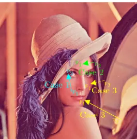
Figure 4.1: Three possible NPD cases to be represented.
Thresholds: Introducing quadratic thresholds
Common decision trees have only one threshold as the splitting decision strategy (Θ< f). Therefore, onlyfirst order information contained in the features is taken into account. For the cases of featuresNPD and Haar only two structures can be learned:
fmin≤f ≤Θ<0≤fmax (4.1)
fmin≤0<Θ≤f ≤fmax (4.2)
Where f is the evaluated feature and fmin and fmax are the feature minimum and
maximum possible values. For NPD f = I(p1)−I(p2)
I(p1)+I(p2) where I(p1), I(p2) are two pixels intensity values. For Haarf =K(p) whereK(p) is a Haar kernel evaluated with its left top corner at the pixel pof the sample.
To exemplify the formulas lets analyze the NPD feature f = I(p1)−I(p2)
I(p1)+(p2). Equation 4.1 is translated as pixelp1 is notably darker than pixel p2. Equation 4.2 is the opposite,
p2 notably darker thanp1. The problem with this representation is that is not possible
to express “high contrast with uncertain polarity”. It is very important that we rep-resent this case because it is desired to be able to reprep-resent an edge between face and background no matter if the background is brighter or darker than the face.
The only way to represent all three cases (see Figure4.1) is to use a quadratic splitting strategy:
af2+bf+c <Θ, where f is the feature (4.3)
In this way, the feature space is divided by a parabola instead of a line. In a practical way, instead of learninga,b,cthe two second order threshold f ∈[Θ1,Θ2] are learned:
fmin ≤Θ1≤f ≤Θ2 ≤fmax (4.4)
This can also be applied to Haar features.
To find the optimal Θ1 and Θ2, for each possible feature dimension we compute a
histogram ofN bins representing the feature value and the weight of the training sample as voting value. Then, over the histograms we perform an exhaustive search optimizing the splitting criterion between the training samples falling inside vs outside of the regions defined by the thresholds.
Classification Result: Measure of the certainty of the windows label
At the end of the face training process, all leafs of the Decision Tree have a set of positive and negative training samples that have fallen into them. It can be seen as a set of histograms of booth positive and negative training samples each representing one of the leafs of each tree. Commonly, for a given windows to be classified, a Decision Tree returns as the classification result the label with more frequency at the node where it has fallen. Another common return value is the probability of the positives training samples at the fallen node. In our implementation the returned value is a measure of the certainty of the windows label, where h(x) ≈1 represents being very sure that the windows is a face, h(x)≈ −1 that it is not a face and h(x)≈0 random guess. Which is expressed as the difference between the weighted probability of the windows of being positive and being negative.
h(R) = w+−w−
w++w− ∈[−1,1] (4.5)
whereRis the region of interest (roi, windows) evaluated andw+,w− are the weights of the positive and negative training samples that fall during training into the leaf where the windows to be evaluated has fallen.
Classification Error as Splitting Criterion
To train the threshold of the Decision Tree (splitting criterion)entropy is normally used. This function is evaluated millions of times: for each possible configuration{Θ1,Θ2} of
each possible feature dimension of each node of each tree. Hence this function must be very fast and highly optimized.
To improve the training velocity, the criterion function was changed from entropy to
MSE (Mean Square Error). Where the MSE of a node Sj is the sum of the MSE of its
left son SjLand right son SjR:
M SE(Sj) =
�
i∈{L,R}
M SE(Sji) (4.6)
where the MSE of a son nodeSji is computed as:
M SE(Sji) =w+(h(Sji)−1)2+w−(h(Sji) + 1)2 (4.7)
wherew+,w−are the positive and negative weights of the training samples falling to the son nodeSij.
Computing this splitting criterion is 6 times faster than computing the Information Gain. With this change, the total training time was reduced almost 30% and the clas-sification rate over the validation set only decreased∼ −2.3%. This is a very important improvement because training time is a critical factor when cross-validating.
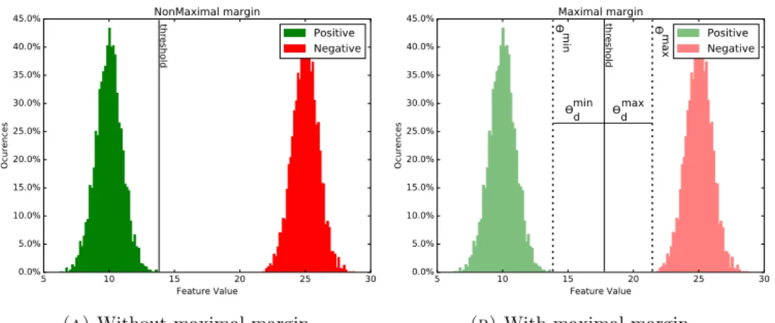
Approximate Maximum Margin
The common Decision Tree splitting criterion is given as the result of an optimiza-tion problem tofind just the maximum information gain, equivalently, in our proposed method,finding the minimum mean square error. This strategy behaves poorly forflat regions of global minima. It is illustrated with the simple example in Figure4.2. This behaviour is not desired. By setting the threshold close to one of the training samples cluster, the model is becoming very sensible to noise. Small changes produced by noise of that cluster will easily cross the threshold and as a consequence be misclassified.
thr
esho
ld
(a)Without maximal margin.
thr esho ld ϴ d min ϴ d max ϴ min ϴmax
(b)With maximal margin.
Figure 4.2: Approximate maximal margin.
To solve this problem, and being inspired by an SVM, we propose to change the decision tree splitting criterion so that it tries to maximize the margin. To do so, we introduce to the optimization problem a constraint to maximize the distance between connected global minimums, minimize Θ1,Θ2 e(Θ1,Θ2) = � i∈{L,R} M SE(Sji)
subject to Θmax1d =Θmin1d ,Θmax2d =Θmin2d
(4.8)
where SL
j,SjR are the two sons of nodeSj and Θmaxd , Θmind are the distances from the
threshold to the maximum and minimum connected global minimums positions in the 1-dimensional solution space (see Figure4.2).
4.2
Soft Cascade
As seen in Section 3.3, traditional Soft Cascade is designed in two stages. First, train the model with AdaBoost. Second, calibration of the model. In the tuning step a new set of calibration samples not previously seen by the classifier is used tofind each weak classifier threshold. This approach has two problems. First, it needs a big dataset (training+calibration+validation+test). Second, the training samples are not being rejected by the learned cascade thresholds which causes that the n-th weak classifier is being trained with samples that the weak classifiers [1, n−1] were able to reject. Thus, the learned weak classifiers are not specialized but general. In this section is presented our proposed solution to solve these problems and new extensions to make it more robust.
Tuning Thresholds in the Training Stage
It is complicated to generate a big and rich dataset of multiple-view faces for training. It is really difficult and time consuming to get a large number of samples of some of the views. It is not desirable to require an extra set of instances just to calibrate the cascade thresholds. Thus, we propose that the thresholds are learned during the training phase, after each weak classifier is trained, so just using the training set.
This change would normally decrease the classifier classification rate. However, it is compensated by improving the algorithm to chose the thresholds using SVM (presented in the next subsection). Moreover, by peaking the thresholds on line, the training samples moving to the next weak classifier to be trained are better selected. Those whose cumulative score is lower than the learned threshold are not used to train the new one. In this way, the new weak classifier is only trained with the kind of training samples that the previous weak classifiers were not able to properly classify. Thus, the classifiers are more specialized and can better filter specific regions of the feature space of faces vs not faces that its predecessors did not explore/specialize on.
Choose cascade thresholds with SVM
As previously explained in Section3.3, the common strategy to select the thresholds is to set the maximum accepted false negatives training samples to be rejected at each step and set the threshold as the maximum possible value that satisfies the constraint. The decision of the threshold values have a direct critical implication to the classification rate. Thus, this standard greedy algorithm is too simple and we propose to set it using machine learning.
Machine learning is very good to make simple decisions based on a lot of rich data. Hence, instead of choosing the threshold values with a greedy algorithm we use a one-dimensional linear SVM. To find the threshold θt of the current stage t, the current
positive and negative sample scores are introduced to the SVM as the one-dimensional feature training samples of booth labels positive and negative. Then the SVM is trained and from the learned model we extract the cascade thresholdθ as:
θ=−b
Notice that w is a number and not a vector because it is a one dimensional SVM, b is the bias. The idea with a cascade of classifiers at a given stage t is to try not to reject any windows being a face and hope that the false positive will be discarded by the following stages [t+ 1, T] (T being the total number of classifiers). During testing the threshold should let pass almost all positive samples. To achieve this behaviour the SVM is learned imposing a much higher weight value to the positive training samples.
During training do not reject samples close to the threshold
Changes of position and illumination of a sample may change the score of that sam-ple. Thus, at a given stage, a testing samples close to the threshold may sometimes be discarded and sometimes not because of small changes of position, orientation and illumination. To make the cascade more robust to this case, during training the 5% of the training samples under the threshold are not rejected. In this way, the next learned weak classifiers will be more robust to these training samples. Then during testing, if testing samples located in the same region of the feature space pass the current stage due to noise, the next weak classifier will have been trained to deal with this kind of samples.
4.3
AdaBoost
Due to the proposed changes of the weak classifiers and the cascade, new optimizations can be introduced to the AdaBoost algorithm to improve the classification rate.
Not Thresholded Weak Classifiers
As seen in Section 3.1, common AdaBoost approaches use weak classifiers in the from h(x)∈{±1}, ht(R) = +1, iff ≥θ −1, otherwise (4.10)
where R is the region of interest (roi, windows). In this form the classification score is given by αt. Our weak classifiers are of the form h(R) ∈ [−1,+1] where its value
value we would be losing valuable information. Therefore, our weak classifiers maintain the range h(R)∈[−1,+1].
Weights Depend on the Threshold
By having the thresholds computed online during the learning phase also helps to im-prove the training samples weight update at each boost iteration. Let us first analyze the current state-of-the-art AdaBoost loss function:
L(H) = N � s=1 e−ms (4.11) with ms=ys T � t=1 αtht(Xs) (4.12)
where N is the number of training samples, T the number of weak classifiers, ms the
voting margin and Xs the sample. What it does is to maximize positive scores while
minimizing at the same time the negatives scores. By having this score behaviour, negative windows will fall under the threshold and as a consequence, rejected.
However, on simple example it can be seen that miss-performs in simple scenarios (see Figure 4.3). Imagine two samples of the training set. During the training process, the negative sample has an absolute value score lower than the positive sample at all the weak classifiers. Thus, given the equation to update the weights derived from the traditional loss function is wts =wst−1e−ysαtht(xs) the negative sample had a higher weight at each
weak classifier. The problem appears when in the calibration stage the chosen threshold happens to be closer to the positive sample rather than to the negative sample due to the rest of the dataset. The weight of the positive sample should have been higher than the negative one on all the weak classifiers, but instead the opposite was done. In other words, during the training stage all weak classifiers have been focusing on the wrong training sample.
To solve this problem we propose to use the fact that the proposed method learns the thresholds on line during the training phase. Instead of just trying to maximizing/mini-mizing the scores, add the constraint that the maximization/minimization of the scores
Figure 4.3: Problem with traditional AdaBoost loss function.
must be relative to the threshold. To express this the voting margin is updated to:
ms =ys( T
�
t=1
αtht(xs)−θt) (4.13)
and as a consequence the equation to update the training samples wights its also updated to
wst =e−ys(�ti=1αihi(xs)−θt) (4.14)
which can be rewritten as
wts= w
t−1
s e−ys(αtht(xs)−Δθ)
N (4.15)
WhereΔθ=θt−θt−1 and N is a normalization factor to ensure �Ss wts= 1.
4.4
Strong Classi
fi
er as a Final Filter
Inspired by theJoint Cascade [16] method, a post-processed classifier to filter the most challenging windows has been added as the post-processing stage of the cascade structure (see Figure3.4). This posterior strong classifier is a learned SVM for each one of the face viewpoints with our own vectorized version of HoG (histogram of oriented gradients) with SIMD instructions (see Section 4.5). The learned SVM is linear to be able to maintain the real time factor.
This finalfilter is just temporal, we are currently working in finding a better one. The problem with this filter is that it requires labeling of the clusters viewpoints and this is not desired for our learning method. However, in experimentation (se Section7.6) it has been shown that only 1% of the windows require the execution of thisfilter.
4.5
Modern and Highly Optimized Code with SIMD
In-structions
Modern CPU include SIMD instructions to accelerate 3D graphics and audio/video pro-cessing in multimedia applications. These instructions allow parallelism at a data level by allowing to perform the same operation to multiple data in a single machine instruc-tion. Notice that this is not concurrency. It is parallel because multiple computations are being done in parallel but only in a single process.
For example, let’s suppose a piece of code for a sequence of array calculations:
floata[8],b[8],c[8]; //... put values into arrays for(inti= 0;i<10;i++){
c[i] =a[i] +b[i]∗1.5f; }
This code can be vectorized with SIMD instructions:
Vec8f avec,bvec,cvec; //... put values into vectors cvec=avec+bvec∗1.5f;
Vec8f vectors are of type m256 which represents a 256-bit vector register holding 8 floating point numbers of 32 bits each. The first code will generate approximately 44 instructions depending on the compiler. However, the vectorized code are only 2 machine instructions with AVX instructions and 4 if the set instructions are SSE2. The difference is caused because the the maximum vector register size of SSE2 instructions is half as big of AVX.
With this simple code optimization we achieved a speedup of 22 for AVX instruction and of 11 for SSE2 instructions. This optimization plus applying other modern C++ code techniques where one of the main reason that made the detector run at 2ms during testing with images of 1080p.
Features
In this chapter a theoretical and computational description of the implemented features is presented.
5.1
Haar-like features
Haar-like features are the most common used features for face detection. They are a set of local appearance kernel each representing a pair of two-dimensional Haar functions. The intuition is to have a set of rectangles-composed kernel describing the difference of pixels intensity between the rectangles in a given position and scale of the region of interest.
Many different kernels have been proposed in literature [1,26,27]. The kernel confi gura-tions are not random at all. Each configuration is defined with the purpose of describing different properties of a region of interest such us edges, lines and surroundings. An example of these descriptions is presented in Figure 5.1. For rotated face, we have also introduced 45 degrees rotated kernels [27].
Each kernel is composed byK rectangular shaped areas with an assigned weight each. Its value is computed as:
f = K � k=1 wk N � i=1 M � j=1 I(i, j) (5.1)
wherewkis the weight of thekth rectangle of dimensionsN×M andI(i, j) the intensity
Figure 5.1: Haar-like kernels feature description. Algorithm 2 Integral Image.
Require: Original Image of N×M size
Ensure: Integral Image ofN ×M size
1: proceduregenerateIntegralImage(I) 2: II(1,1) :=I(1,1); 3: fori=1 in N do 4: forj=1 inM do 5: II(i, j) :=I(i, j) +II(i, j−1) +II(i−1, j)−II(i−1, j−1); 6: end for 7: end for 8: end procedure
To evaluatefapplying directly the presented Equation5.1has a high computational cost because the intensity sum of overlapping areas is recomputed multiple times by different kernel. In practice, instead of applying Equation 5.1 an Integral Image is calculated and used to rapidly evaluate f at any scale and position with O(1) complexity. It is computed as, II(i, j) = �i s=1 �j t=1I(s, t), if 1≤i≤N and 1≤j≤M 0, otherwise (5.2)
whereN andMare the number of rows and columns of the original imageIrespectively. TheIntegral Image has been computed with the Algorithm2with linear timeO(N×M). By using Integral Image, querying the sum of intensity pixels in a rectangular area can be performed with O(1) complexity as,
I(p1, p2) =II(p1.y, p1.x)−II(p1.y, p2.x)−II(p2.x, p1.y) +II(p2.y, p2.x) (5.3)
WhereP1 represent the top left point andP2 the bottom right point of the rectangular region. For a fast computation of the rotated kernels, a rotated Integral Image is also generated.
In this project it was NOT used a predefined set of kernels. Instead, a total number of 78900 kernels were generated and then accepted or rejected by applying boost. To generate these kernels a set of 14 templates were deformed by width and height and set in all possible positions that feet in the region of interest.
5.2
Normalized Pixel Di
ff
erence
The Normalized Pixel Difference (NPD) is a very simple but yet elegant local feature based on comparison of pixel intensities. It is value is computed as the normalized difference of pixel intensity between two points (see Figure5.2),
f(p1, p2) =
I(p1)−I(p2) I(p1) +I(p2)
(5.4)
whereI is the intensity value and p1 and p2 two given pixels. For grey-scale images of I ∈[0,255] NPD is a bounded nonlinear function f(p1, p2) ∈[−1,1]. If we analyze the
formula that what this feature is returning a vector which its module is the percentage of joint intensity I(p1)−I(p2) and its sense indicates the ordinal relationship between
booth pixelsp1, p2.
f
Figure 5.2: Normalized pixel difference representation.
NPD is a very elegant feature because despite of its apparent simplicity it has a lot of desirable properties. First, the vector module is symmetric, for boothI(p1)−I(p2) and I(p2)−I(p1) its value is the same, only its sense changes. Hence, the future space is
which have a feature space of (N(N××MM−)!2)! where N ×M are the number of pixels of the region of interest.
Second, the sign of the NPD (its vector sense) indicates the ordinal relationship between booth evaluated pixels. In literature [28,29] it has been shown that ordinal relationship is a good indicator for object detection because it describes the intrinsic structure, in other words, it describes a given part of an object with respect to the others. However, this property is highly sensitive to noise for pixels of similar intensity. For example, beingp1 = 6, p2 = 7 the feature value is easy to change between positive and negative
signs due to small changes in illumination. This issue has been solved by introducing second order thresholds in the decision tree. This is explained with further detail in Section 4.1.
Third, invariant to scale changes of pixels intensity. For features with this simplicity it Is practically impossible tofind a feature which is invariant to any light variation in the region of interest. However, by being scale invariant to pixels intensity it is expected to have some level of robustness in front of changes of illumination.
Fourth, its previously explained [−1,1] bound makes it perfectlyfitted for threshold and histogram based learning methods such us decision trees which are the selected weak classifier representation.
For a fast computation,T255x255look-up table is precomputed, where rows represent all
possible values ofI(p1) and columns all possible values of I(p2). Hence, given a couple
of pixels, its NPD value can be queried with complexity O(1) as T(p1, p2). Although
having the same computational complexity as a Haar feature, only one query to a matrix is required vs 4 queries for HAAR.
5.3
Histogram of Oriented Gradients
Histogram of oriented gradients (HoG) is a commonly used feature for object detection. It describes the shape of an object as a distribution of its intensity gradients. The image is divided into small spatial regions called cells each containing n×n pixels. For each cell a histogram of its pixels gradient directions is computed and normalized to make it
more robust to illumination and shadowing. Thefinal descriptor is the concatenation of the normalized histograms of each block (group of cells).
First, the horizontal∂x(x, y) and vertical∂x(x, y) image gradients are computed. To do
so, thederivative masks is applied over the image in the vertical and horizontal direction.
[−1,0,1] and [−1,0,1]� (5.5)
Second, for each pixel in the image its gradient magnitude and orientation are computed.
m(xi, yi) = � ∂x(xi, yi)2+∂y(xi, yi)2 (5.6) Θ(xi, yi) =arctan � ∂y(xi, yi) ∂x(xi, yi) � (5.7) Then each cell histogram is generated. Histograms x coordinate represent the angle of the gradients which can be unsigned ([0◦,180◦]) or signed ([0◦,360◦])s). Each pixel within the cell falls into a bin of the histogram based on its gradient orientation and casts a weighted vote for that orientation equal to its gradient magnitude.
To improve robustness against illumination and shadow changes a normalization factor is applied to large spatial regions. In other words, normalization is applied over groups of cells named blocks which overlap so each cell contributes to multiple blocks. There are different possible block normalization techniques, the one used consists on computing the L2-norm (Equation 5.8) and then clipping the values and re-normalize,
h
�
�h�22+c2
(5.8)
wherev represents the histogram andc a constant. The final descriptor is the concate-nation of the normalized histograms.
Temporary planning
In this Chapter the definition of tasks and their temporal scheduling plan are defined.
6.1
Tasks identi
fi
cation
The development of this project will be performed usingAgilemethodologies. Hence, the project is divided into a set of tasks (iterations) each one divided in analysis, implemen-tation, testing, integration and documentation. The application of agile methodologies will allow a more close up feedback relationship with the project supervisors as well as a faster response against obstacles and incidents.
6.1.1 State of the art and learning
In this first task an evaluation of the current state of the art will be analyzed. The objective of this task is to identify the most promising state of the art training algorithms, features and classifiers which do/could fulfill the established detector constraints. Once identified, study all the necessary theory in order to understand and be able to implement the method.
6.1.2 Debugging dataset generation
Search and filter an on line frontal face dataset to be used for initial debugging of the classifier, features and learning algorithm.
6.1.3 Learning classifier
Once decided in the State of the art this task states the classifier to be used. Its implementation must be highly modular and reusable because different features and learning algorithm would be tested on it. Also, it is not desired to implement it with low level optimizations as multiple version and changes could be made in future iterations. The classifier must be as transparent as possible. To achieve this transparency a set of scripts to plot the current state of the classifier will be implemented.
6.1.4 Features
Implement, test and evaluate all identified features that could be used. All features must have the same interface for modular and reusable purposes. In this way, changing between features does not affect any of the other modules.
6.1.5 Learning algorithm
Implementation and testing of the learning algorithm to train the classifier. Learning algorithms tend to be a black box. It is desired to make this step as transparent as possible. To do so, a set of scripts to plot the state of each step of the learning process must be implemented.
6.1.6 Final dataset generation
Once the classifier is properly being trained, a rich, wellfiltered dataset will be generated. It is intended to implement a script to scratch the web, downloading face pictures and then implementing a program to fast label each sample. The labeling will consist of defining the face bounding box and position configuration.
6.1.7 Classifier training and validation
In this step the classifier will have to be implemented by cross-validating all the critical parameters.
6.1.8 Classifier implementation optimization
Once the classifier and the features to be used have been decided, highly optimize the code. Run a code profiler to identify the most critical parts of the code an apply modern low-level compiler optimizations.
6.1.9 Final documentation
At each iteration the documentation of that task will be generated. Hence, in thisfinal iteration onlyfinal polishes over the documentation will be made.
6.2
Time estimation
In Figure6.1a time estimation of each task/iteration is presented.
Task Time Estimation
Task/Iteration Time [h]
State of the art and learning 168
Debugging dataset generation 25
Learning classifier 168
Features 168
Learning algorithm 420
Final dataset generation 24
Classifier training and validation 96 Classifier implementation optimization 213
Final documentation 20
TOTAL 1289
Figure 6.1: Gannt diagram initial planning
6.3
Initial planing
At CMU a researcher works 12 hours and 7 days a week. As a Visiting Scholar this timetable is also applied to me. Hence, all the planning has been calculated with an estimated 84 hours of full dedication to this project every week. The visiting period is 22 weeks. A Gantt planning diagram can be seen in Figure6.1.
6.4
Final planning
In the initial planning it was defined that only 48 hours would be necessary to generate the dataset of samples. This estimation was based on the supposition that the laboratory would proportionate it. Then, it would only be necessary to clean it and adapt it to our necessities. However, the laboratory did not have any dataset that fitted our needs. It was necessary to hand-label 200K faces of multiple viewpoints which took one week.
Figure 6.2: Gannt diagramfinal planning.
As previously explained, this project has been managed with agile methodologies which allow to check and adapt dynamically the initial planning. Thus, a modification of the initial planning was made. Hours of optimization where moved to generate the dataset. With this new planning the number of code optimizations and tricks decreased but all the initial objectives where achieved. The new gantt diagram is presented in Figure6.2.
Task Time Estimation
Task/Iteration Time [h]
State of the art and learning 168
Debugging dataset generation 25
Learning classifier 168
Features 168
Learning algorithm 420
Final dataset generation 168
Classifier training and validation 84 Classifier implementation optimization 84
Final documentation 20
TOTAL 1285
Experimentation and results
Every time a new model is learned with new updates and upgrades a battery of tests are executed to validate the model. Moreover, this unit tests generate a sequence of plots to try to transform the black box classifier into a white box classifier. In this chapter, some of these plots are presented.
All these experiments have been performed with the same model configuration which used NPD features. The one with better classification rate found so far. The learning algorithms take 20 minutes to learn the model in a 20 cores Intel Corporation Xeon E7 v2/Xeon E5 v2/Core 3GHz sever without GPU.
The model has been trained with a dataset of 101241 positive samples and 305203 negative ones. 80% of the samples have been used to cross-validate and 20% to test. There are more negative samples than positives because of bootstrap.
7.1
Proof of concept - basic tests
Figure 7.1: Two linearly separable basic test with two featuref ∈[0,255]. The radius
of each sample represents its weight.
Figure 7.2: First nonliear basic test with two featuref ∈[0,255]. The radius of each
sample represents its weight.
The proposed classifier introduces a lot of changes over the traditional methods on which it is based on. Thus, it has been tested over a set of simple linearly and nonlinear separable datasets in a 2-dimensional space as an initial proof of concept.
Figure 7.3: Second nonliear basic test with two feature f ∈ [0,255]. The radius of each sample represents its weight.
First, it was tested with two simple linearly separable datasetes (see Figure7.1). Notice how the thresholds are able to maximize the margin between clusters thanks to the proposed modification of the decision trees splitting criterion.
The proposed classifier was also tested with more difficult nonlinear samples (see Fig-ure7.2and Figure7.3). To make the plots more understandable, all presented examples have been trained with the classifier constrained to learn one level decision trees. The radius of the samples (circles) represent the weight of each sample.
As it can be seen, the classifier is able to learn a nonlinear model to correctly classify non-linear separable samples. Notice how at each step the weight associated to misclassified instances increase so that the following classifier take them more into consideration.
7.2
Learned cascade decision trees
With the objective of making the classifier as transparent as possible we developed a script to plot a representation of the weak classifiers (see Figure 7.4). Each node of the tree contains the following information: ID of the selected feature, number and weight