Classifying Cancer Genomic Alterations Using Machine Learning and Multi-Omic Data

(1)

UC Santa Cruz

UC Santa Cruz Electronic Theses and Dissertations

Title

Permalink

https://escholarship.org/uc/item/14h4h24s

Author

Haan, David

Publication Date

2019

License

CC BY-NC-ND 4.0 Peer reviewed|Thesis/dissertation

(2)

UNIVERSITY OF CALIFORNIA SANTA CRUZ

CLASSIFYING CANCER GENOMIC ALTERATIONS USING MACHINE LEARNING AND MULTI-OMIC DATA

A dissertation submitted in partial satisfaction of the requirements for the degree of

DOCTOR OF PHILOSOPHY in

BIOMOLECULAR ENGINEERING & BIOINFORMATICS by

David Haan September 2019

The Dissertation of David Haan is approved:

Professor Josh Stuart, Chair

Professor Angela Brooks

Professor Christopher Benz

(3)

Copyright cby David Haan

(4)

List of Figures

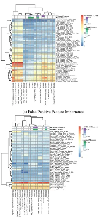
3.1 Boruta Feature Importance Analysis By Fusion Submission.Heatmap

show-ing results from performshow-ing the Boruta algorithm on each submissions false positive fusion events(A) and false negative fusion events(B). Each cell in the heatmap represents the Z-score Mean Decrease in Accuracy. Higher Z-scores are in red and represent more important features. Rows are the fusion submis-sion names and columns are the features. Only features which had a mean value

greater than Borutas shadow max value are shown. . . 15

3.2 Boruta Feature Importance Analysis Across All Fusion Submissions for

the False Positive Model(A) and False Negative Model(B). Boxplot

show-ing results from performshow-ing the Boruta Algorithm on all fusion submissions. The y-axis represents the Z-score MDA and features are across the x-axis. The red plots are the Z-scores of the actual features and blue are Borutas shadow features which are considered the randomized background features. Only

fea-tures which performed significantly better (p< .05) than the shadow features

(7)

3.3 False Negative Feature Analysis T Statistic. Students t-test of top features identified by False Negative Random Forest model. Students t-test was per-formed individually on the 5 features comparing false negative fusions missed by the submission methods to the accurately identified fusions. A negative t

statistic represents a decrease in the feature values for false negative fusions. . 17

4.1 REVEALER results of using IDH1 positive control test sets. Each column

represents the samples in the TCGA Lower Grade Glioma (LGG) dataset. The top row is the classifier score assigned to each sample using an initial classifier trained on the first IDH1 test set of 150 samples. The tick marks in the seed row represent the 150 IDH1 test set samples. REVEALER identified 4 matches, ATRX truncating mutations, TP53 missense mutations, and a 11p15.5 focal deletion. While these are not invalid results as it has correctly found genes

(8)

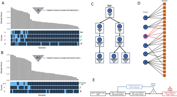
4.2 LURE Method. (A) LURE Oncoprint of Bait Mutation A.Triangle symbol represents the classification model for samples having event A. Barplot show-ing the score given to each sample by the model representshow-ing the probability the sample has the mutation event A. The annotation bars below indicate mutations present in each sample. The check mark annotations on the right mark if events passed Sample Set Enrichment Analysis (SSEA, see Supplemental Methods)

(p< .05, fdr< .25). (B) LURE Oncoprint of Intermediate Bait Mutation

A:C.Results from a classification model containing both events A and C.(C)

LURE Event Discovery Tree. Directed graph shows LURE’s iterative Event

Discovery Tree. Each node is a classification model built on the events shown in the triangle symbol within each node. The blue circles within each node

rep-resent the newest event added to the model. (D) LURE Set Cover Algorithm.

Bipartite graph shows the result of running a Set Cover Algorithm on the mu-tations collected from the Event Discovery Tree and the samples predicted to be mutated in these genes by the final classification model. The red node and edges mark Event F, which is completely overlapping with other mutations and

therefore removed from the final event set (’Catch’ Cover).(E) LURE Method

(9)

4.3 LURE Bait and Catch Oncoprints of positive controls. Samples are rep-resented across the rows. Colored tick marks represent the different types of alterations present in the samples. Barplot on top shows the LURE classifier

score for each sample after the final iteration. (A) SF3B1 test set in UVM.

Initial bait is set to 8 SF3B1 missense in UVM, and LURE finds the 2 left out

sets of 5 each. (B) IDH1 test set in LGG.Initial bait is set to 150 samples of

IDH1 Missense in LGG and Lure finds the 3 left out sets of 20 each. . . 25

4.4 Histogram of Bait Precision-Recall Area Under the Curve. Plot shows a

his-togram of the 3,053 Precision Recall AUC cross validation scores from training a tumor type specific logistic regression classifier on the different 723 COSMIC genes. Classifiers were created only in tumor types with more than 10 alterations. 27

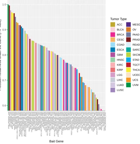
4.5 Barplot of 81 Bait Classifiers. Barplot shows Precision-Recall AUC test scores

for 81 bait-tumor type classifiers. Bar is colored by tumor type. . . 28

4.6 Heatmap of baits used in PANCAN LURE analysis. Rows are bait and

al-teration type, and the columns are tumor type. Each cell in the heatmap cor-responds to the PR AUC score of that bait/alteration/tumor type classifier. The higher scoring baits are in red/orange and blue denotes no classifier due to lack of alterations in that bait tissue combination. TP53 was the most common bait across tissues and the tumor types with highest number of high scoring baits

(10)

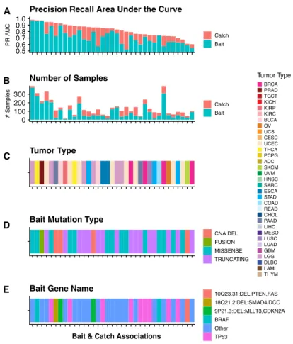
4.7 Bait Catch Association Data Panel. Panel shows bait and catch annotations for the 35 baits in which associations were found. Baits are across the x-axis and

sorted by final Bait and Catch PR AUC.(A) Precision Recall Area Under the

Curve. Stacked bar plot shows the original PR AUC score of the bait and the

final PR AUC score including the new catch.(B) Number of SamplesStacked

bar plot shows the number of samples in the bait and the additional samples in

the catch. (C) Tumor Type. Annotation bar shows the tumor type in which

the bait-catch association was found.(D) Bait Mutation Type. Annotation bar

shows the type of bait mutation. (E) Bait Gene Name. Annotation bar shows

the name of the bait gene. . . 31

4.8 High Confident LURE PANCAN Results. Sankey plot shows the high

con-fident 18 bait-catch associations with a final PR AUC greater than 0.8. Bait gene and mutation type are on the left side and the Catch bait gene and muta-tion type are on the right side. The flows represent an associamuta-tion between the bait and catch gene. The color of the left side of each flow is the tumor type in which each association was found. The color of the right side of each flow is

the association type. . . 32

4.9 LURE ”Event Net” of LURE PANCAN ResultsLURE Event Net shows all

associations resulting from the 35 successful cosmic bait genes. Edges are col-ored by the tumor type in which the association was found. Edges are directed

(11)

4.10 LURE Oncoprint and Survival Plot. (A) Using a known driver for ALT, ATRX truncating mutations, for bait in Sarcomas(SARC), LURE found three

catch events: copy number deletions in ATRX, RB1, and SP100. (B)Survival

plot shows the ALT classification using the final set cover classifier from the

LURE method. . . 36

4.11 MAPK LURE Pathway Analysis (A) LURE ”Event Net” showing MAPK/RTK

associations. Each node represents an event. The directed edges represent an

association and the direction of the LURE discovery. The color of each edge

represents the tumor type in which the association was found. (B) LURE

On-coprint of HRAS in HNSC.Using HRAS as a bait in HNSC, LURE found a

delection catch event of the 2q23.3 region. . . 38

4.12 Alluvial Plot of LURE PCAWG Results. The left side of the plot shows the

Baits and the right side shows Catches. The flow represents the tumor type in

(12)

5.1 Overview of the pathway and network analysis approach. Coding, non-coding, and combined gene scores were derived for each gene by aggregating driver p-values from the PCAWG driver predictions in individual elements, in-cluding annotated coding and non-coding elements (promoter, 5 UTR, 3 UTR, and enhancer). These gene scores were input to five network analysis algo-rithms (CanIsoNet [Kahraman et al., in preparation], Hierarchical HotNet, an induced subnetwork analysis [Reyna and Raphael, in preparation], NBDI, and SSA-ME), which utilize multiple protein-protein interaction networks, and to two pathway analysis algorithms (ActivePathways [Paczkowska, Barenboim et al., in submission] and a hypergeometric analysis [Vazquez]), which utilize multiple pathway/gene-set databases. We defined a non-coding value-added (NCVA) procedure to determine genes whose non-coding scores contribute sig-nificantly to the results of the combined coding and non-coding analysis, where NCVA results for a method augment its results on non-coding data. We defined a consensus procedure to combine significant pathways and networks identi-fied by these seven algorithms. The 87 pathway-implicated driver genes with coding variants (PID-C) are the set of genes reported by a majority ( 4/7) of methods on coding data. The 93 pathway-implicated driver genes with non-coding variants (PID-N) are the set of genes reported by a majority of methods on non-coding data or in their NCVA results. Only 5 genes (CTNNB1, DDX3X,

(13)

5.2 Overlap of consensus results for pathway and network methods. (A) PID-C

and PID-N genes have negligible overlap. Only 5 genes (CTNNB1, DDX3X,

SF3B1, TGFBR2, TP53 are both PID-C and PID-N genes. (B) Overlap of all

consensus results. Four-circle Venn diagram for the overlap of the consensus

results on coding data, i.e., PID-C genes; consensus pathway/network results on coding data; consensus pathway/network results on coding and non-coding data; and the union of the consensus results on non-non-coding data and the

(14)

5.3 Pathway and network modules containing PID-C and PID-N genes. (A)

Network of functional interactions between PID-C and PID-N genes.Nodes

represent PID-C and PID-N genes and edges show functional interactions from the ReactomeFI network (grey), physical protein-protein interactions from the BioGRID network (blue), or interactions recorded in both networks (purple). Node color indicates C genes (green), N genes (yellow), or both PID-C and PID-N genes (orange);node size is proportional to the score of the cor-responding gene; and the pie chart diagram in each node represents the rel-ative proportions of coding and non-coding cancer mutations associated with the corresponding gene. Dotted outlines indicate clusters of genes with roles in chromatin organization and cell proliferation, which predominantly contain PID-C genes; development, which includes comparable amounts of PID-C and PID-N genes; and RNA splicing, which contains PID-N genes. A core cluster of genes with many known drivers are also indicated. (B) Pathway modules containing PID-C and PID-N genes. Each row in the matrix corresponds to a PID-C or PID-N gene, and each column in the matrix corresponds to a pathway module enriched in PID-C and/or PID-N genes (see Methods). A filled entry indicates a gene (row) that belongs to one or more pathways (column) colored according to gene membership in PID-C genes (green), PID-N genes (yellow), or both PID-C and PID-N genes (orange). A darkly colored entry indicates that a PID-C or PID-N gene belongs to a pathway that is significantly enriched for PID-C or PID-N genes, respectively. A lightly colored entry indicates that a PID-C or PID-N gene belongs to a pathway that is significantly enriched for the union of PID-C and PID-N genes but not for PID-C or PID-N genes separately. Enrichments are summarized by circles adjacent each pathway module name and PID gene name. Boxed circles indicate that a pathway module contains a pathway that is significantly more enriched for the union of the C and PID-N genes than the PID-C and PID-PID-N results separately. The enriched modules and PID genes are clustered into four biological processes: chromatin,

(15)

5.4 RNA splicing factors are targeted primarily by non-coding mutations and alter expression of similar pathways as coding mutations in splicing fac-tors. (A) Heatmap of Gene Set Enrichment Analysis (GSEA) Normalized

Enrichment Scores (NES).The columns of the matrix indicate non-coding

mu-tations in splicing-related PID-N genes and coding mumu-tations in splicing genes reported in [1] and the rows of the matrix indicate 47 curated gene sets[1]. Red heatmap entries represent an upregulation of the pathway in the mutant samples with respect to the non-mutant samples and blue heatmap entries represent a downregulation. The first column annotation indicates mutation cluster mem-bership according to common pathway regulation. The second column annota-tion indicates whether a mutaannota-tion is a non-coding mutaannota-tion in a PID-N gene or a coding mutation[1], with the third column annotation specifies the aberration type (promoter, 5 UTR, 3 UTR, missense, or truncating). The fourth column annotation indicates the cancer type for coding mutations from [1]. The mu-tations cluster into 3 groups: C1, C2, and C3. The pathways cluster into two groups[1]: P1 and P2, where P1 contains an immune signature gene sets and P2

contains cell autonomous gene sets as reported in [1]. (B) tSNE plot of

mu-tated elements illustrates clustering of gene expression signatures for sam-ples with non-coding mutations in splicing-related PID-N genes with gene expression signatures for coding mutations in previously published

splic-ing factors. The shape of each point denotes the mutation cluster assignment

(C1, C2, or C3), and the color represents whether the corresponding gene is a

(16)

5.5 Cluster stability analysis. (A)Silhouette scores of pathway clusters 1 and 2. Silhouette width is on the x-axis, and the 47 pathways across y-axis. Average

silhouette score per cluster is shown to the right of the bar plots.(B)Silhouette

scoring of the 3 mutation element clusters.(C, D)Histograms representing the

results of a cluster bootstrapping analysis using the Jaccard similarity coefficient

to identify how often pathways(C)or mutation elements(D)clustered together

in each bootstrap. . . 49

5.6 Differences between normal and cancer-associated telomere properties.

Scat-ter plot showing the four clusScat-ters of telomere patScat-terns identified across PCAWG cancers, together with the more homogeneous cluster of matched normal

sam-ples, generated by t-Distributed Stochastic Neighbour Embedding. . . 52

5.7 Telomere sequence patterns across PCAWG. (A) Scatter-plot showing the

four clusters of telomere patterns identified across PCAWG by t-Distributed Stochastic Neighbour Embedding (tSNE). (B) Distribution of the four clusters of telomere patterns in selected tumour types from PCAWG. (C) Distribution of relevant driver mutations associated with alternative lengthening of telomere and normal telomere maintenance across the four clusters. (D) Distribution of telomere maintenance abnormalities across tumour types with more than 40 patients in PCAWG. Samples classified as tumour cluster 1-3 if they fall into a relevant cluster without mutations in TERT, ATRX or DAXX and have no ALT

(17)

5.8 Properties of telomeres across different tumor clusters. (A) Distribution of telomere sequence and properties across samples in the four clusters, with both tumour (blue points) and matched normal (red points) shown. (B) Enrichment (positive T statistics) or depletion (negative T statistics) of different variant se-quence motifs in the four clusters of telomere properties. (C) Variance of

fre-quency of different sequence motifs across the four clusters. . . 55

5.9 Properties of telomeres across different normal clusters.Properties of

telom-eres across different normal clusters. Enrichment (positive T statistics) or de-pletion (negative T statistics) of different variant sequence motifs in the four

normal clusters of telomere properties. . . 56

5.10 Co-mutation and expression levels of genes related to telomere

mainte-nance across the four clusters of telomere properties. (A) Patterns of

co-mutation of the relevant driver co-mutations across individual patients. Columns in plot represent individual patients, coloured by type of abnormality observed. (B) Box and whisker plots of expression levels of key telomere maintenance genes across the four clusters of telomere properties. The boxes demarcate the

interquartile range, with a horizontal line to mark the median. . . 57

5.11 Timing of mutation in genes related to telomere maintenance.Clonal [early]

denotes clonal mutations occurring before duplications involving the relevant chromosome (including whole genome duplications); clonal [late] to clonal mu-tations occurring after such duplications; and clonal [NA] to mumu-tations

(18)

Abstract

Classifying Cancer Genomic Alterations Using Machine Learning and Multi-Omic Data

by David Haan

In 2018, an estimated 1,762,450 new cases of cancer will be diagnosed in the United States and 606,880 people will die from these diseases. Cancer is a group of diseases characterized by the overgrowth of abnormal cells as the result of genomic mutations. Mutations that initi-ate tumorigenesis are called driver mutations whereas those which cannot are called passenger mutations. Driver mutations define a tumor’s subtype and can be used as therapeutic targets thus, deciphering driver mutations from passenger mutations is of utmost importance as we strive to improve cancer treatment. As the cost of genome sequencing is decreasing, the amount of available tumor data is increasing, making it possible to conduct large scale computational analysis with machine learning to identify novel tumor characteristics. There have been nu-merous recent collaborations to collect, sequence, and analyze human tumors. The largest of these collaborations, the Cancer Genome Atlas (TCGA), is a comprehensive analysis of 9,000 patients and 33 sub types cataloging mutation data, DNA, mRNA, methylation, and protein expression. Whereas the TCGA is mostly whole exome sequencing, the International Cancer Genome Consortium (ICGC) has begun contributing data from the whole genome sequencing of a few thousand tumors. Using both the TCGA and ICGC data, I performed four new variant

(19)

pervised machine learning technique to identify tumor subtypes, driver mutations and potential therapeutic targets. I first present an analysis in which I used supervised machine learning to determine the most important genomic features responsible for accurate gene fusion detection among a set of fusion detection methods. Next, I present a method of unsupervised machine learning in which I classify non-coding variants of splicing factors as potential driver mutations in a number of tumor types. Third, I analyze telomere data from ICGC whole genome sequenc-ing data ussequenc-ing unsupervised machine learnsequenc-ing to identify 4 subtypes of telomere maintenance mechanisms(TMM) among 2,500 tumor samples. Lastly, I present a new variant classification method called LURE, which uses supervised machine learning to classify variants based on existing signatures from known driver mutations.

(20)

Chapter 1 Introduction

Approximately 39.3 percent of men and women will be diagnosed with cancer of any site at some point during their lifetime[2]. In 2016, there were an estimated 15,338,988 people living with cancer of any site in the United States[2].

Cancer is a genetic disease caused by mutation and selection in somatic cells. Mu-tations in normal cells are usually repaired or result in apoptosis. Whereas in cancer cells mu-tations accumulate, leading to uncontrolled growth and tumorigenesis. There are two broadly defined types of mutations: drivers and passengers. Tumors contain around 2-5 driver mutations that cause and accelerate cancer, and about 10-200 passenger mutations which are accidental byproducts of thwarted DNA repair mechanisms[3]. Driver mutations define key characteris-tics of the tumor and may offer therapeutic targets, yet identifying them amid the myriad of passengers remains a challenge.

The Cancer Genome Atlas (TCGA) is a publicly accessible dataset of cancer samples

(21)

DNA methylation, copy number variation, and protein expression data for roughly 11,000

pa-tients across 33 cancer types[?]. The identification of driver mutations played a fundamental

role in many TCGA analyses. Whereas the TCGA is mostly whole exome sequencing, the In-ternational Cancer Genome Consortium (ICGC) has begun contributing data from the whole genome sequencing of a few thousand tumors. Using both the TCGA and ICGC data, I per-formed four new variant classification analyses using both unsupervised machine learning tech-niques and a novel supervised machine learning technique to identify tumor subtypes, driver mutations and potential therapeutic targets.

There are two types of machine learning methods: supervised and unsupervised. Un-supervised learning methods, such as hierarchical clustering and T-distributed Stochastic Neigh-bor Embedding(t-SNE), are effective at visualizing high dimensional data and identifying clus-ters or patterns in the data[4]. Supervised machine learning uses prior knowledge or labels to divide data into two or more classes[4]. By training a classification model on prior knowledge, supervised machine learning can make predictions about unknown or unlabeled data[4]. In this thesis, I present unsupervised and supervised machine learning methods I performed on cancer genomic data to classify mutations or variations found in the genomes of human tumors.

In chapter 3, I recapitulate my participation in a bioinformatics community challenge ranking user-submitted gene fusion detection methods. In this challenge, we spiked gene fusion transcripts into a few human cancer cell lines and asked participants to run their own gene fusion detection methods on these datasets. I was tasked with performing analysis on the data to determine if the presence of certain genomic features near a fusion prevented methods from detecting the fusion. After collecting a set of genomic features for each fusion, I used a random

(22)

forest, a supervised machine learning method, to predict the false positive and false negative fusion events called by each method. I then preformed a feature importance analysis to identify the genomic features responsible for each method’s incorrect fusion detection.

Next, I sought to classify mutation variants by developing a supervised machine learn-ing tool called Learnlearn-ing UnRealized Events (LURE). LURE, discussed in chapter 4, associates alterations between samples by finding similar signatures in feature data, such as mRNA ex-pression data or methylation data. LURE achieves this by training a classifier on tumor sample feature data of a known driver mutation (the bait), applying the classifier to find ”bait”-absent samples with a high classifier score, and identifying other alterations (the ”catch”) in those sam-ples that correlate with the high classifier score. Using LURE, I identify new associations across pan-cancer data and find putative new driver alterations involved with MAPK signaling. In ad-dition, I associate new driver alterations with the alternative lengthening of telomeres (ALT), a telomere maintenance mechanism (TMM), in sarcomas.

In chapter 5, I discuss variant classification of non-coding mutations using supervised learning. First, using hierarchical clustering of pathway expression data, I relate non-coding mutations of splicing factors with coding mutations of the same splicing factors. Next, using t-SNE on telomere related features, I identify 4 unique groups of tumor samples that employ different TMMs and associate mutations with each of these groups. In chapter 6, I outline conclusions based on my research and discuss the future directions of cancer genomics.

(23)

Chapter 2 Background

2.1 Cancer is a Genetic Disease

Cancer is a genetic disease typically resulting from an accumulation of mutations[3]. Mutations in normal cells generally result in repair or cell suicide. However, in cancer cells, the mutations accumulate leading to an uncontrolled growth otherwise known as a tumor. There are two broadly defined types of mutations, driver and passenger mutations. Tumors contain around 2-5 driver mutations which cause and accelerate cancer, and about 10-200 passenger mutations that are accidental byproducts of thwarted DNA repair mechanism. Driver mutations define a tumor’s subtype and can be used as therapeutic targets.

2.2 The Cancer Genome Atlas

TCGA (cancergenome.nih.gov) is a publicly accessible collection of data from the NCI[5]. This atlas of data is a comprehensive analysis of 9,000 patients and 33 cancer subtypes

(24)

cataloging mutation data, DNA, mRNA, methylation, and protein expression[5]. The majority of the TCGA data is whole exome sequencing that covers only protein coding regions of the genome[5]. As the cost of sequencing is decreasing, whole genome sequencing of numerous and diverse patient samples has become more practical. This has enabled the creation of the PanCancer Analysis of Whole Genomes (PCAWG), a data base of 2,500 patient-derived tumor sequencing profiles of various cancer subtypes[6].

2.3 Mutation Types

There are numerous types of mutations and other genetic alterations that directly ini-tiate tumorigenesis[3]. Single nucleotide variations (SNVs) result from the insertion, deletion or subsitution of a single nucleotide and are the most common genomic mutations. SNVs in non-coding regions of the genome can result in aberrant activity of promoters, enhancers, and silencers. SNVs in coding regions are typically single nucleotide substitutions that change a three-base amino acid codon sequence resulting in either the production of the same amino acid (silent mutation), a different amino acid (missense mutation), or a stop codon (truncating muta-tion). Missense and truncating mutations are more deleterious because they change the amino acid composition of a protein. Insertions and deletions of nulceotides in the coding sequences can also affect protein composition by causing a frameshift mutation that typically results in an early stop codon and thus, a truncated protein product. Copy number alterations are large deletions or amplifications of a genomic region that result in either decreased or excessive pro-tein production. Gene fusions occur when two genes at the DNA level are joined through a

(25)

translocation, interstitial deletion, or chromosomal inversion and produce a chimeric protein.

2.4 Machine Learning

There are two types of machine learning: unsupervised and supervised. Unsupervised machine learning is a method that finds new patterns in a dataset without pre-existing labels and is typically used in cancer genomics to identify subtypes or clusters of tumors that share a sim-ilar set of features. Supervised learning is used when a computer algorithm cannot be used to solve a given problem without implementing example data or previous experiences[7]. A super-vised machine learning method builds a model by defining a set of features and labels for each data point or observation in an example dataset. There are many types of supervised machine learning such as linear regression, logistic regression, random forest and neural networks.[7]. To illustrate the utility of supervised machine learning, consider an example in which a logistic regression model is used to distinguish between different species of flowers. The length and width of the sepals and petals may be considered flower features and the flower species (a label) is assigned to each flower based on their specific features. The model is trained on this existing data, known as training data, and can be used to further predict the species of a new flower given its sepal and petal measurements. In this thesis, I present my work based on similar prin-ciples of machine learning to determine a tumor’s mutation status based on gene expression or methylation data and determine which features are most important for tumor classification.

(26)

2.5 Modeling Imbalanced datasets

Biological data is often imbalanced, leading to difficulty in building accurate clas-sification models. In cancer genomic data, there is more data collected from tumors of par-ticular subtypes, usually those subtypes exhibiting well-studied genetic mutations, like PTEN or BRCA. This leads to misleading analysis results when metrics are not weighed per class. For example, when using such data to classify multiple different tumor subtypes, a model may achieve better overall accuracy by classifying both the larger and smaller classes as the larger class. Thus, it is imperative that the correct accuracy metric is chosen to avoid a false depiction of good accuracy. The Receiver Operating Characteristic Area Under the Curve (ROC AUC) is a very popular metric but is highly inaccurate for imbalanced models because it relies on the true positive rate and false positive rate, the later being weighted for the negative class[8]. Overall, this results in the inaccurate measurement of false positives. To further explore the cause of this defect, imagine classifying a dataset with a 5-95 (true-false) split. If the classifier guessed all 5 true positives as positive but classified 5 false positives as positive as well, then the false positive rate for the ROC curve would be 5/95, or 0.0526, which is very low. Although only 0.0526 of the negative class was incorrectly classified, equal numbers of samples were guessed wrong as were guessed right therefore, this classification is unreliable. Usually in the case of imbalanced classes, there is more concern with how well the classifier can identify the smaller class or classes. When trying to model a rare genetic mutation, accurately determining the mutated samples is crucial for analysis while the negative class is of little interest. In this situation, it is best to use precision and recall to measure accuracy of imbalanced classification

(27)

models because they are weighted for only the positive class. Precision is a measure of the false positives that is weighted for the positive class. This quantifies how often a model incorrectly guessed a negative label as a positive per the number of true positive samples. In the example above where the false positive rate was only 0.0526, the precision is 0.5 (false positives/(correct true positives+false positives)). With a precision of only 0.5, it would most likely be necessary to discredit the classification model. Recall is the true positive rate; it measures how often the model accurately identifies the positive labels as positive per the number of true positives. To-gether, these two metrics can be used to create either an F1 score, which is the harmonic mean of precision and recall, or a precision-recall area under the curve(PR AUC)[8]. When classify-ing imbalanced datasets, precision-recall AUC or F1 scores can be used to add a description of the model’s accuracy.

2.6 Driver Discovery Tools

There are several existing computational tools that try to decipher driver from passen-ger mutations[9]. EPoC uses network modeling of the transcriptional effects of copy number aberrations to identify driver mutations in glioblastoma (GBM)[10]. DriverNet employs a prob-abilistic model to locate driver mutations using transcriptional networks[11]. These methods can predict novel drivers given a set of SNVs or copy number alterations and the corresponding mRNA gene expression data. In addition, there are methods that identify modules of driver genes based on mutual exclusivity in certain tumor types, such as CoMEt[12] and MEMo, the latter of which incorporates prior knowledge such as pathway data into driver gene module

(28)

(29)

Chapter 3 Accurate Fusion Detection

3.1 Introduction

Genomic rearrangements in cancer cells produce fusion transcripts that may give rise to protein products not present in normal cells. These can serve as robust diagnostic markers, e.g. TMPRSS2-ERG in prostate cancer[14] or drug targets, e.g. BCR-ABL1 in chronic myeloid leukemia[15]. Ongoing research efforts are beginning to unveil the potential clinical relevance of aberrant processing of RNA in cancer, such as defects in alternative-splicing. An assortment of computational methods are needed to fully document the transcriptomic differences between tumor cells and their normal counterparts. Increasing the alterome of tumors by fully character-izing their RNA landscapes will expand our understanding of cancer mechanisms, provide new biomarkers and reveal possible new RNA-based therapeutics, improving personalized patient treatment.

(30)

translo-cation, interstitial deletion, or chromosomal inversion. A fusion may also occur at the RNA level, resulting from a ligation between two transcripts. Gene fusions often play an important role in the initial steps of tumorigenesis. Specifically, gene fusions have been found to be the driver mutations in neoplasia and have been linked to various tumour subtypes. An increasing number of gene fusions are being recognized as important diagnostic and prognostic parameters in malignant haematological disorders and childhood sarcomas. Reviews have estimated that gene fusions occur in all malignancies and that 20% of human cancer cases harbour at least one to RNA fusion events[16, 17].

The goal of this challenge is to use a crowd-based competition to identify the opti-mal methods for quantifying isoforms and detecting mRNA fusions from RNA-seq data. Sev-eral methods have been published that detect and quantify cancer-associated RNA abundance species. Yet, it is not clear which methods are best used and under what contexts. Recent systematic comparisons have been performed[18, 19] to evaluate RNA-Seq analysis methods. Most comparisons have been performed by an author of one of the competing methods and so may suffer self assessment bias. One of the more recent evaluations, performed by an impartial list, was the study by Kumar et al 2016 that compared 12 different methods based on their accu-racy, length of execution time, and memory requirements. The work performed by the authors in Creason, et al, includes several newly developed tools, the use of spike-ins for an unbiased assessment of sensitivity, an objective evaluation framework in which the administrators ran submitted methods to generate all predictions, and a statistical procedure to infer background fusions to accurately measure precision. In addition to a new evaluation of methods, our work provides a tool for simulating RNA isoforms and fusions, a new benchmark dataset against

(31)

which forthcoming methods can be compared, and all of the tested methods in standardized workflow for re-execution, which should further progress this area of study. My contribution to the community challenge was to rank the isoform challenge and run a feature importance pipeline on the fusion detection methods.

3.2 Dream Challenge Results

The fusion detection evaluation challenge received 63 entries, of which the organizers were able to run 37. The final evaluation consisted of 17 entries, which included multiple sub-missions by the same team (up to three per team allowed). Two different datasets were created to evaluate methods-a computationally simulated dataset and another experimentally generated set using spike-ins (Figure 2a). The simulated dataset was used to evacuate the preliminary rounds. The simulated data were generated with the program rnaseqSim (in preparation) that created synthetic reads from computationally constructed fusions. On average, the simulated tumor samples contained 39 fusions per transcriptome. The second evaluation dataset of spike-ins was used for the final evaluation of methods. The spike-in data were created in the lab using a prescribed series of fusion products spiked in to several cancer cell lines, using 18 different fusion constructs. Scoring of the fusion methods was performed using the F1 score against the spike-in set. To account for fusions found in the cell line background, fusions called by mul-tiple methods across mulmul-tiple replicates were collected for PCR based validation, and utilized as an imputed truth set to augment the spike-in set (see methods). An additional F1 score was calculated for the combined (spike-in plus imputed) truth set. All submitted entries were ranked

(32)

according to their F1 score on the combined data. Two of the submitted methods emerged as the overall winners of this sub-challenge – Arriba and STAR-Fusion – based on their perfor-mance in spike-in benchmarks with the addition of the imputed truth set. Arriba achieved an F1 of 0.73, and STAR-Fusion had an F1 of 0.70. The next closest entry, another permutation of STAR-Fusion, was at 0.63. Based on a bootstrap analysis, no other methods were found to have achieved results as accurate as these top two entries. The next method, not submitted by one of the winning teams was fusioncatcher, submitted by the challenge administrators, at 0.58. Finally, the highest scoring method, not submitted by the top two teams or the administrators, was STAR-SEQR with an F1 of 0.47.

3.3 Features Influencing the Accuracy of Fusion Detection

Meth-ods

In an effort to determine what factors influence methods to incorrectly call fusion events, I created a fusion feature importance pipeline, similar to what was done for the SMC-DNA challenge[20]. To start, I collected 128 genomic features for each predicted fusion event, including gene length, transcript length, distance from the breakpoint to repeats, and the abun-dance for each fusion partner. Next, I built a random forest (RF) classification model to predict the false-positive fusion events from each submission. The RF was trained to select features that predict when a method erroneously calls a fusion event when no such event was present according to the i-truth. Also, I built a second RF model to select features that predict false negative events; i.e. the RF predicts when a method fails to detect a spiked-in fusion construct.

(33)

To determine feature importance among our classification models I applied our random forest models to the algorithm Boruta, an all relevant feature selection algorithm[21][22](Figure 3.1). Boruta determines feature relevance by comparing the original importance with the importance achievable at random, estimated using permuted versions of a feature, and progres-sively eliminating irrelevant features to stabilise the test. In order to determine the features most relevant to all the methods, Iincluded the submission ID as a feature and created one false positive classification model achieving an out-of-bag (OOB) error rate of only 0.26%. The false negative RF model was more difficult to predict due to fewer observations, but achieved an error rate of 7.64%. The Boruta algorithm revealed that the number of transcripts and GC content were the most important features for determining the false positives among all fusion methods whereas submission id, coverage across junction and expression were the top fea-tures for the false negative model(Figure 3.2). Further analysis of the top feafea-tures for the false negative model revealed a marked decrease in coverage and expression for the false negative fusions(Figure 3.3).

3.4 Conclusion

Here I presented some of the results of the SMC-RNA DREAM challenge in which we synthetically introduced fusions and asked contestants to run fusion detection methods and report the results. Through my feature importance analysis I determined that coverage, expres-sion, GC content, and the number of transcripts of each fusion partners are the most important features. Identifying alterations in tumor sequence data is very important, but even more so is

(34)

8399080_ST ARSEQRv050_merged_ 8040408_genomehack er_w or kflo 9609498_smcFusion_Her a_w or kf 9609499_smcFusion_Her a_w or kf 8645203_uhr igs−smc−r na−fusio 9609502_uhr igs−smc−r na−fusio 8645601 8645625 8281648_Winterf ell Fusion F e 8396553 9609508_uhr igs−smc−r na−fusio 8114525 9610272_ST ARSEQRv060_merged_ 8517255_fusioncatcher_1 8644608_F o xtrot 9610021_smcFusion.Ma y2017.Wi Unknown_repeats_1500_2000 scRNA_repeats_2000_2500 LINE_repeats_0_500 DNA_repeats_2000_2500 last_partner_last_exon DNA_repeats_500_1000 DNA_repeats_1000_1500 DNA_repeats_1500_2000 LTR_repeats_500_1000 LTR_repeats_1500_2000 LINE_repeats_2000_2500 Simple_repeat_repeats_2000_2500 LTR_repeats_1000_1500 cell_line LTR_repeats_2000_2500 LTR_repeats_0_500 DNA_repeats_0_500 Simple_repeat_repeats_1500_2000 Low_complexity_repeats_1500_2000 Simple_repeat_repeats_500_1000 Low_complexity_repeats_500_1000 Low_complexity_repeats_2000_2500 Simple_repeat_repeats_0_500 LINE_repeats_500_1000 LINE_repeats_1500_2000 Low_complexity_repeats_1000_1500 first_partner_first_exon LINE_repeats_1000_1500 SINE_repeats_2000_2500 SINE_repeats_1500_2000 Low_complexity_repeats_0_500 Simple_repeat_repeats_1000_1500 SINE_repeats_0_500 SINE_repeats_500_1000 SINE_repeats_1000_1500 Acceptor_GC_content_w_introns Acceptor_GC_content_wo_introns Donor_Num_Transcripts_1 Donor_GC_content_wo_introns Donor_Gene_Size Donor_Trscpt_Size_w_introns Acceptor_Num_Transcripts_2 Acceptor_Num_Exons Donor_Expression Donor_Num_Exons Donor_GC_content_w_introns Acceptor_Expression Acceptor_Gene_Size Acceptor_Trscpt_Size_w_introns Donor_Trscpt_Size_wo_introns Acceptor_Trscpt_Size_wo_introns Actual.F1.score FP.Model.F1.score FP.Model.F1.score 0.95 0.85 Actual.F1.score 0.75 0.5 0 5 10 15 20 25 30 35

(a) False Positive Feature Importance

8040408_genomehack er_w or kflo 8114525 8399080_ST ARSEQRv050_merged_ 9610272_ST ARSEQRv060_merged_ 8517255_fusioncatcher_1 9609498_smcFusion_Her a_w or kf 9609499_smcFusion_Her a_w or kf 8281648_Winterf ell Fusion F e 9610021_smcFusion.Ma y2017.Wi 8645601 8645625 8645203_uhr igs−smc−r na−fusio 9609502_uhr igs−smc−r na−fusio 8644608_F o xtrot 8396553 9609508_uhr igs−smc−r na−fusio LTR_repeats_500_1000 Acceptor_Trscpt_Size_w_introns Acceptor_Trscpt_Size_wo_introns Donor_GC_content_w_introns Acceptor_GC_content_w_introns Donor_Trscpt_Size_wo_introns Donor_Gene_Size Donor_Trscpt_Size_w_introns Donor_Num_Transcripts_1 Acceptor_Gene_Size Acceptor_GC_content_wo_introns Acceptor_Num_Exons Donor_Num_Exons Donor_GC_content_wo_introns SINE_repeats_1500_2000 Acceptor_Num_Transcripts_2 LTR_repeats_2000_2500 LINE_repeats_0_500 LTR_repeats_1500_2000 DNA_repeats_1000_1500 Low_complexity_repeats_1000_1500 Low_complexity_repeats_500_1000 DNA_repeats_1500_2000 spiked_in_amt SINE_repeats_500_1000 LINE_repeats_1500_2000 DNA_repeats_500_1000 Low_complexity_repeats_0_500 LINE_repeats_1000_1500 SINE_repeats_1000_1500 SINE_repeats_2000_2500 LINE_repeats_500_1000 SINE_repeats_0_500 LINE_repeats_2000_2500 Junction_Coverage Donor_Expression Acceptor_Expression Donor_Coverage Acceptor_Coverage Actual.F1.score FP.Model.F1.score FP.Model.F1.score 0.92 0.86 Actual.F1.score 0.65 0.4 0 5 10 15 20 25

(b) False Negative Feature Importance

Figure 3.1: Boruta Feature Importance Analysis By Fusion Submission. Heatmap

show-ing results from performshow-ing the Boruta algorithm on each submissions false positive fusion events(A) and false negative fusion events(B). Each cell in the heatmap represents the Z-score Mean Decrease in Accuracy. Higher Z-scores are in red and represent more important features. Rows are the fusion submission names and columns are the features. Only features which had a mean value greater than Borutas shadow max value are shown.

(35)

● ● ● ● ● ● ● ● ● ● ● ● ● ● ●● ● ● ● ● ● ● ● ●●●●●● ● ● ● ● ● ● ● ● ● ● ● ● ● ● ● ● ● ● ● ●●●● ● ● ●●●●●●●●● ● ● ● ● ● ● ● ● ●●●●● ● ● ● ● ●●● ● ● ● ● ● ● ● ● ● ● ● ● ● ● ● ●●●● ● ● ● ● ● ● ● ● ● ● ● ● ● ● ● ● ● ● 0 20 40 Random_Min Random_MeanRandom_Max LTR_repeats_0_500 Unkno wn_repeats_1500_2000LTR_repeats_1000_1500 scRNA_repeats_2000_2500 Lo w_comple xity_repeats_1500_2000 DNA_repeats_0_500 LTR_repeats_2000_2500LTR_repeats_500_1000 Simple_repeat_repeats_2000_2500 LTR_repeats_1500_2000 last_par tner_last_e xon Lo w_comple xity_repeats_2000_2500 DNA_repeats_500_1000 DNA_repeats_1500_2000 DNA_repeats_2000_2500 first_par tner_first_e xon Simple_repeat_repeats_1500_2000Simple_repeat_repeats_500_1000 DNA_repeats_1000_1500 Simple_repeat_repeats_0_500 LINE_repeats_1500_2000 Lo w_comple xity_repeats_500_1000 SINE_repeats_1000_1500 LINE_repeats_2000_2500 LINE_repeats_0_500 submission_id Lo w_comple xity_repeats_1000_1500 LINE_repeats_1000_1500 Simple_repeat_repeats_1000_1500 SINE_repeats_2000_2500 SINE_repeats_0_500 SINE_repeats_500_1000 LINE_repeats_500_1000 cell_line Donor_Gene_Siz e Acceptor_Num_Exons SINE_repeats_1500_2000 Donor_T rscpt_Siz e_w_introns Acceptor_Num_T ranscr ipts_2 Lo w_comple xity_repeats_0_500 Acceptor_T rscpt_Siz e_w_introns Donor_GC_content_w_introns Donor_T rscpt_Siz e_w o_introns Donor_Expression Acceptor_Gene_Siz e Acceptor_T rscpt_Siz e_w o_introns Acceptor_Expression Donor_GC_content_w o_introns Donor_Num_Exons Donor_Num_T ranscr ipts_1 Acceptor_GC_content_w o_introns Acceptor_GC_content_w_introns Feature Z−score MD A Category Actual Random

(a) False Positive Feature Importance

● ● ● ● ● ● ● ● ●●●●●● ● ● ● ● ● ● ● ● ● ● ● ● ● ● ●● ● ●● ● ● ● ● ● ● ● ● ● ● ● ●● ●● ● ● ●● ● ● ● ● ● ●●● ●●● ● ● ● ● ● ● ● ● ● ● ● ● ● ● ● ● ● ● ● ● ● ● ● ● ● ● 0 10 20 30 40 Random_Min Random_MeanRandom_Max DNA_repeats_0_500 Lo w_comple xity_repeats_1500_2000 Simple_repeat_repeats_500_1000 last_par tner_last_e xon Simple_repeat_repeats_2000_2500 LINE_repeats_1000_1500 Lo w_comple xity_repeats_0_500 DNA_repeats_2000_2500 first_par tner_first_e xon

DNA_repeats_1500_2000DNA_repeats_500_1000SINE_repeats_1000_1500 LINE_repeats_1500_2000

SINE_repeats_0_500

spik

ed_in_amt

DNA_repeats_1000_1500 SINE_repeats_1500_2000 SINE_repeats_500_1000

Lo w_comple xity_repeats_500_1000 SINE_repeats_2000_2500LINE_repeats_500_1000 LINE_repeats_0_500 LTR_repeats_1500_2000 Lo w_comple xity_repeats_1000_1500 LINE_repeats_2000_2500 LTR_repeats_2000_2500 L TR_repeats_500_1000 Acceptor_T rscpt_Siz e_w_introns Acceptor_Num_Exons Acceptor_Num_T ranscr ipts_2 Acceptor_Gene_Siz e Donor_GC_content_w_introns Donor_GC_content_w o_introns Acceptor_GC_content_w o_introns Donor_Num_Exons Acceptor_T rscpt_Siz e_w o_introns Donor_Gene_Siz e Donor_Num_T ranscr ipts_1 Donor_T rscpt_Siz e_w_introns Acceptor_GC_content_w_intronsDonor_T rscpt_Siz e_w o_intronscell_line Acceptor_Co v er age Donor_ExpressionDonor_Co v er age Acceptor_ExpressionJ unction_Co v er age submission_id Feature Z−score MD A Category Actual Random

(b) False Negative Feature Importance

Figure 3.2: Boruta Feature Importance Analysis Across All Fusion Submissions for the

False Positive Model(A) and False Negative Model(B). Boxplot showing results from

per-forming the Boruta Algorithm on all fusion submissions. The y-axis represents the Z-score MDA and features are across the x-axis. The red plots are the Z-scores of the actual features and blue are Borutas shadow features which are considered the randomized background

fea-tures. Only features which performed significantly better (p< .05) than the shadow features

are shown in this plot.

determining if these alterations would be considered drivers and contribute to tumorigenesis. Is it possible that a fusion event is capable of driving cancer? What other events could be driving cancer and how can we identify them?

(36)

−25 −20 −15 −10 −5 0 Acceptor_Co v er age Donor_Expression Donor_Co v er age Acceptor_Expression J unction_Co v er age Feature T Statistic

Figure 3.3: False Negative Feature Analysis T Statistic. Students t-test of top features

iden-tified by False Negative Random Forest model. Students t-test was performed individually on the 5 features comparing false negative fusions missed by the submission methods to the ac-curately identified fusions. A negative t statistic represents a decrease in the feature values for false negative fusions.

(37)

Chapter 4 LURE: Classifying Coding Variants of

Unknown Significance

LURE (Learning UnRealized Events): Finding New(or Equivalent) Driver Mutation Events using Supervised Machine Learning

4.1 Introduction/Background

There are several existing computational tools that try to decipher driver from passen-ger mutations[9]. EPoC uses network modeling of the transcriptional effects of copy number aberrations to identify driver mutations in glioblastoma (GBM)[10]. DriverNet employs a prob-abilistic model to locate driver mutations using transcriptional networks[11]. These methods can predict novel drivers given a set of SNVs or copy number alterations and the corresponding mRNA gene expression data. In addition, there are methods that identify modules of driver genes based on mutual exclusivity in certain tumor types, such as CoMEt[12] and MEMo, the

(38)

latter of which incorporates prior knowledge such as pathway data into driver gene module discovery[13]. In contrast, LURE uses mRNA data to identify mutations in “driver-unknown” samples with similar expression signatures to known drivers, thereby implicating a novel set of mutations as possible drivers.

Several studies have built gene expression signatures to identify samples with certain driver events. For example, studies have identified a TP53 gene expression signature as a re-liable and independent predictor of disease outcome in breast cancer[23, 24]. In addition, in patients with epithelial ovarian cancer, a BRCAness gene expression signature is just as pre-dictive of chemotherapy responsiveness and outcome as mutation status.[25] While creating signatures as prognostic markers to guide treatment is important in a clinical setting, there has been little work using such gene expression signatures to find related mutational events. LURE identifies gene expression signatures across the 723 COSMIC cancer genes[26] and then uses iterative semi-supervised learning to discover potentially related events.

A similar method, REVEALER is a computational method that identifies combina-tions of genomic alteracombina-tions correlated with functional phenotypes, such as the activation or gene dependency of oncogenic pathways or sensitivity to a drug treatment[27]. While the con-cept of REVEALER is very similar to LURE, there are few differences which make LURE better. For one, at every iteration of the process LURE produces a new classification model slightly more accurate than the previous as the newly discovered events are no longer false positives and now aide in determining features relevant to the signature. Second, REVEALER utilizes a mutual exclusive relationship between new events which may limit results as muta-tion calls are not 100% accurate. Allowing some overlap between predicted events LURE can

(39)

account for possible mutation call errors and identify modules containing co mutated events. In an effort to compare methods, my undergraduate mentee, Ruikang Tao ran REVEALER using one of our test sets described in our positive controls and REVEALER was unable to identify the leave-out test sets (Supplemental Figure 4.1).

4.2 Method

LURE attempts to associate alterations between samples by finding similar signatures in feature data such as mRNA expression data. LURE achieves this by training a classifier using the samples of a known driver mutation (the bait) applying it to find ”bait”-absent samples with a high classifier score, and looking for other alterations (the ”catch”) in those samples that correlate with the high classifier score.

The first step (Step 0) is to establish a known driver mutation as the initial bait, for example event A (Figure 4.2A,E). In the next step (Step 1) LURE trains a logistic regression classification model using gene expression as features and bait mutation status as the label to be predicted. A cross-validation is run for the classification task and baits can be filtered by model performance, e.g. area under the precision recall curve (PR AUC). LURE then uses the classification model to score each sample in the dataset (Figure 4.2A,E). Notwithstanding the inherent bias towards overfitting, there might be some negative samples not mutated in the bait gene that still receive a high classifier score. These false positives from the classification task show the same expression signal as the bait-mutated samples hinting to a different driver event having a similar effect on the cancer cells.

(40)

REVEALER − Iteration: 1 TARGET: LGG IC / CIC SUMMARY SEED: 0.75 SEED: IDH1_test_set1_set1 0.75 Top 4 Matches CARS_del 11p15.5 HRAS_del 11p15.5 TP53_missense 17p13.1 ATRX_truncating Xq21.1 CIC p−val FDR 0.2 <7e−05 0 0.21 <7e−05 0 0.25 <7e−05 0 0.25 <7e−05 0

TCGA.S9.A89Z TCGA.P5.A5EU TCGA.TM.A84M TCGA.HT

.7606

TCGA.S9.A6TZ TCGA.FG.A4MX TCGA.DU.6396 TCGA.HT

.7608 TCGA.DU.7306 TCGA.HT .7693 TCGA.HT .7684 TCGA.VM.A8CB TCGA.R Y .A840

TCGA.DH.A7UU TCGA.DU.7007TCGA.S9.A7J0 TCGA.DH.A66D TCGA.DU.7010 TCGA.R

Y

.A83Z

TCGA.S9.A6UB TCGA.HT

.A61B

TCGA.DU.6410 TCGA.FG.5965 TCGA.E1.A7Z6 TCGA.DB.5279 TCGA.S9.A7R3 TCGA.HW

.8322

TCGA.S9.A7J1 TCGA.DH.5142 TCGA.HT

.8563

TCGA.DU.A76O TCGA.QH.A6X4 TCGA.DB.A64X TCGA.P5.A737 TCGA.TM.A84H TCGA.E1.A7Z4 TCGA.P5.A77XTCGA.HT

.7601

TCGA.DB.A4XF TCGA.DU.5855 TCGA.FG.6690TCGA.E1.5322 TCGA.DU.5872 TCGA.CS.5394 TCGA.TM.A84T TCGA.DH.A66F TCGA.DB.A75KTCGA.HT

.7686

TCGA.DU.8164 TCGA.QH.A870 TCGA.TQ.A7RN TCGA.DU.6400 TCGA.S9.A7QWTCGA.WY

.A858

TCGA.TM.A84G TCGA.FG.A4MT TCGA.VV

.A829

TCGA.DH.A7US TCGA.QH.A65Z TCGA.E1.A7YE TCGA.P5.A72Z TCGA.VV

.A86M

TCGA.DU.6542 TCGA.DU.6408 TCGA.R8.A6ML TCGA.DB.A64U TCGA.TQ.A7R

U

TCGA.R8.A6MO TCGA.TQ.A7R

W

TCGA.E1.A7YV TCGA.DU.6397 TCGA.DH.5144 TCGA.R8.A6MK TCGA.DH.A669 TCGA.S9.A7J3 TCGA.HT

.7873

TCGA.CS.5390 TCGA.DU.7008 TCGA.FG.A60L TCGA.QH.A6X9 TCGA.HT

.A615

TCGA.HW

.7490

TCGA.CS.4942 TCGA.DU.7294 TCGA.DB.5273 TCGA.S9.A7R1 TCGA.S9.A7R8 TCGA.R

Y

.A83Y

TCGA.S9.A7IYTCGA.P5.A5EW TCGA.TM.A84STCGA.HT

.7616

TCGA.TQ.A7RH TCGA.DU.6395 TCGA.TM.A7CATCGA.HT

.7677

TCGA.HT

.8108

TCGA.HW

.8319

TCGA.FG.8186 TCGA.DU.A5TR TCGA.S9.A6U1 TCGA.S9.A6TV TCGA.WY

.A85C

TCGA.P5.A781 TCGA.E1.5304TCGA.VW

.A7QS

TCGA.FG.8185 TCGA.WY

.A85A

TCGA.TM.A84OTCGA.E1.5307 TCGA.TM.A84I TCGA.DU.8168 TCGA.CS.6670TCGA.WH.A86K TCGA.TQ.A7RJ TCGA.FG.A711TCGA.FG.A6IZ TCGA.S9.A7R7 TCGA.DU.5870 TCGA.TQ.A8XE TCGA.QH.A6X5 TCGA.FG.A87N TCGA.HT

.7604

TCGA.S9.A6WN TCGA.DB.A64P TCGA.FG.A60K TCGA.DU.8166TCGA.R

Y .A845 TCGA.HT .7483 TCGA.DB.A64Q TCGA.HW .8320 TCGA.S9.A6TU TCGA.HT .7858

TCGA.VM.A8C8 TCGA.DB.5280 TCGA.DU.6394 TCGA.S9.A6TSTCGA.E1.5302 TCGA.FG.7637TCGA.DH.A66G TCGA.P5.A77WTCGA.HT

.7471 TCGA.HT .8106 TCGA.HT .7610 TCGA.TQ.A7RK TCGA.HT .8111 TCGA.HT .8114 TCGA.HT .7690 TCGA.DB.A75M TCGA.HT .7879 TCGA.FG.8188 TCGA.TQ.A7RRTCGA.QH.A6X3TCGA.DU.7015TCGA.FG.A710TCGA.S9.A6WHTCGA.TQ.A7RMTCGA.DB.A64RTCGA.E1.5305TCGA.HT .A614

TCGA.DB.5276 TCGA.DU.7302 TCGA.P5.A735 TCGA.WY

.A85E

TCGA.DB.5277 TCGA.HT

.A5RB

TCGA.HT

.7485

TCGA.FG.7641 TCGA.FG.A6J3 TCGA.E1.A7Y

O

TCGA.P5.A5EX TCGA.FG.5962 TCGA.CS.6666 TCGA.DU.A76R TCGA.DB.A4XB TCGA.DU.7019 TCGA.TQ.A7RS TCGA.FG.8191 TCGA.WY

.A85D

TCGA.DB.A4X9TCGA.E1.A7YITCGA.DU.A5TU TCGA.TQ.A7RI TCGA.DU.A6S2TCGA.HT

.8105

TCGA.S9.A7J2TCGA.VM.A8CATCGA.HT

.7478 TCGA.HT .7676 TCGA.HT .A74L TCGA.R Y .A847

TCGA.DU.A5TW TCGA.TM.A84QTCGA.DU.6399 TCGA.S9.A6TX TCGA.P5.A733 TCGA.P5.A5EZ TCGA.FG.6689 TCGA.DH.A7UV TCGA.R

Y

.A83X

TCGA.DU.7298 TCGA.E1.A7YS TCGA.TM.A84L TCGA.HT

.8013

TCGA.DB.A64L TCGA.S9.A6WQ TCGA.DU.7018 TCGA.S9.A7QX TCGA.VM.A8CH TCGA.TQ.A7RG TCGA.DU.5853 TCGA.HT

.A618

TCGA.HT

.7482

TCGA.P5.A5ET TCGA.FG.A6J1 TCGA.FG.8187 TCGA.HT

.7470

TCGA.HT

.A74O

TCGA.S9.A6U5 TCGA.DU.A6S7 TCGA.HT

.7480

TCGA.DB.A64V TCGA.E1.A7YK TCGA.S9.A7R4 TCGA.HT

.7884

TCGA.QH.A6CUTCGA.CS.4938 TCGA.HT

.8010 TCGA.HW .A5KL TCGA.FG.6691 TCGA.TQ.A7RQTCGA.HT .7605

TCGA.DH.A66B TCGA.DU.A6S3 TCGA.CS.6665TCGA.S9.A7IZ TCGA.HT

.7475 TCGA.P5.A5F0 TCGA.TQ.A7R V TCGA.S9.A6WD TCGA.HT .7875 TCGA.DU.8167 TCGA.HT .7687

TCGA.DB.5274 TCGA.R8.A73M TCGA.DU.A7T6 TCGA.F6.A8O3 TCGA.DU.5871 TCGA.DB.A64WTCGA.HT

.A74J

TCGA.CS.5396 TCGA.DU.A6S8 TCGA.HT

.7468

TCGA.FG.A4MY TCGA.FG.A70Y TCGA.DU.7304 TCGA.S9.A6U6TCGA.HT

.7902 TCGA.KT .A74X TCGA.R Y .A843 TCGA.QH.A65STCGA.IK.8125 TCGA.HT .7692

TCGA.FG.A60J TCGA.S9.A6U8 TCGA.HT

.7609

TCGA.S9.A6TW TCGA.CS.6290 TCGA.QH.A86X TCGA.HW

.7495

TCGA.DU.8163 TCGA.P5.A72W TCGA.TQ.A7RF TCGA.DU.7299 TCGA.DB.A4XD TCGA.DU.A6S6 TCGA.DB.5275 TCGA.DB.A75L TCGA.QH.A65V TCGA.DB.A4XE TCGA.DB.5281 TCGA.S9.A6WGTCGA.FG.7638TCGA.WY

.A85B

TCGA.TM.A84F TCGA.P5.A5F2 TCGA.HW

.A5KJ

TCGA.P5.A780 TCGA.HT

.7607

TCGA.FN.7833TCGA.DB.A4XC TCGA.QH.A6CZ TCGA.P5.A5EV TCGA.TM.A7C4 TCGA.DB.A4XGTCGA.S9.A7IS TCGA.FG.7634TCGA.DB.A4XHTCGA.DU.A7TI TCGA.DU.5851 TCGA.HT

.A4D

V

TCGA.CS.5393 TCGA.HT

.7481

TCGA.QH.A6CY TCGA.TM.A7C5TCGA.HT

.8018 TCGA.HT .7855 TCGA.HW .8321 TCGA.HT .7611 TCGA.HT .7620 TCGA.HT .8109

TCGA.DH.5143 TCGA.CS.6667 TCGA.FG.7636 TCGA.HT

.A5R7

TCGA.HT

.7881

TCGA.DH.A7UT TCGA.HW

.7493

TCGA.DU.7011 TCGA.F6.A8O4 TCGA.WY

.A859

TCGA.W9.A837 TCGA.DB.A4XA TCGA.P5.A72X TCGA.CS.4943TCGA.HT

.7472

TCGA.DB.A64S TCGA.HT

.8012

TCGA.TQ.A7R

O

TCGA.S9.A6U2 TCGA.S9.A6WP TCGA.HW

.A5KM

TCGA.S9.A6WE TCGA.DU.A7T8 TCGA.DB.5270 TCGA.P5.A5F1TCGA.HT

.7474

TCGA.P5.A731 TCGA.DU.7300 TCGA.HT

.7877

TCGA.DU.A5TP TCGA.QH.A65R TCGA.DU.5849TCGA.HT

.7467

TCGA.HW

.7491

TCGA.DU.A7TC TCGA.S9.A7QZ TCGA.DU.7309 TCGA.P5.A736 TCGA.QH.A6XA TCGA.QH.A6X8 TCGA.P5.A5F4TCGA.HT

.7874

TCGA.E1.A7YH TCGA.HT

.7688

TCGA.P5.A730 TCGA.HT

.A74K

TCGA.E1.5311 TCGA.DH.5141 TCGA.HW

.7489 TCGA.S9.A6W O TCGA.HT .7694 TCGA.HT .A5R9

TCGA.S9.A6TY TCGA.S9.A6U9 TCGA.VM.A8CE TCGA.HT

.7473

TCGA.QH.A65X TCGA.DB.A75O TCGA.E1.A7YW TCGA.HT

.A619

TCGA.TM.A7CF TCGA.E1.A7Z3 TCGA.DU.A5TS TCGA.CS.4944 TCGA.DU.6393 TCGA.DU.7014TCGA.HT

.8113

TCGA.HT

.7479

TCGA.S9.A7QY TCGA.HT

.7681

TCGA.E1.A7YU TCGA.VM.A8CF TCGA.S9.A7IQ TCGA.S9.A6WLTCGA.HT

.7477

TCGA.DH.A7UR TCGA.FG.A713 TCGA.HT

.A5R5 TCGA.HT .7856 TCGA.HT .A616 TCGA.E1.5303

TCGA.TM.A84R TCGA.DH.5140 TCGA.DU.A7T

A TCGA.S9.A6WI TCGA.HT .7603 TCGA.HT .7880 TCGA.HT .8558 TCGA.HT .7476

TCGA.FG.8189 TCGA.E1.A7YY TCGA.TM.A84C TCGA.HT

.A61A

TCGA.DU.A7TG TCGA.DU.8162 TCGA.FG.8181 TCGA.P5.A5EY TCGA.FG.5963TCGA.HT

.8107 TCGA.HT .8015 TCGA.HT .7680 TCGA.FG.7643 TCGA.HT .8019 TCGA.DU.7292 TCGA.HT .7691 TCGA.QH.A6CW TCGA.E1.A7YD TCGA.HT .7469 TCGA.S9.A6WMTCGA.VW .A8FI

TCGA.E1.A7YQ TCGA.QH.A6CX TCGA.S9.A6U

A

TCGA.DB.A75P TCGA.HT

.7854

TCGA.DU.8158 TCGA.FG.A87Q TCGA.DU.5854 TCGA.QH.A6CSTCGA.E1.A7YNTCGA.HT

.A5RC TCGA.HT .A61C TCGA.HT .8110 TCGA.E1.A7YMTCGA.HT .7857 TCGA.HW .A5KK TCGA.CS.5397 TCGA.HT .A74H

TCGA.DU.6402 TCGA.DU.8161 TCGA.DU.7013 TCGA.VM.A8C9 TCGA.S9.A7R2 TCGA.FG.A70Z TCGA.TM.A84J TCGA.DU.7006 TCGA.VM.A8CDTCGA.HT

.A617

TCGA.FG.6688 TCGA.P5.A72U TCGA.KT

.A7W1

TCGA.DU.6404 TCGA.HT

.7882

TCGA.QH.A6XC TCGA.DU.7290 TCGA.P5.A5F6 TCGA.E1.A7YJ TCGA.S9.A89VTCGA.HT

.8564

TCGA.DU.6392 TCGA.DU.5852 TCGA.DU.A7TB TCGA.HT

.A5RA

TCGA.S9.A6U0 TCGA.DU.A76L TCGA.DU.6403 TCGA.FG.6692 TCGA.HT

.A4DS

TCGA.DB.A64O TCGA.DU.7012 TCGA.FG.A4MWTCGA.CS.6186 TCGA.S9.A7IX TCGA.DU.A76K TCGA.E1.A7YL TCGA.DU.A5TY TCGA.HT

.8011

TCGA.TM.A84B TCGA.CS.6188 TCGA.DU.A5TT TCGA.TM.A7C3 TCGA.DU.A7TJ TCGA.DU.8165 TCGA.TQ.A7RP TCGA.DU.6405 TCGA.FG.A4MU TCGA.CS.4941TCGA.HT

.7860

TCGA.QH.A6CV TCGA.E1.A7Z2 TCGA.DU.6406 TCGA.DU.5847 TCGA.DU.A7TDTCGA.HT

.8104

Figure 4.1: REVEALER results of using IDH1 positive control test sets. Each column

represents the samples in the TCGA Lower Grade Glioma (LGG) dataset. The top row is the classifier score assigned to each sample using an initial classifier trained on the first IDH1 test set of 150 samples. The tick marks in the seed row represent the 150 IDH1 test set samples. REVEALER identified 4 matches, ATRX truncating mutations, TP53 missense mutations, and a 11p15.5 focal deletion. While these are not invalid results as it has correctly found genes co-mutated with IDH1, it was unable to find the 60 left out IDH1 mutants.

(41)

Therefore, in Step 2, LURE takes the false positive samples and the rest of the nega-tive samples and runs SSEA (Sample Set Enrichment Analysis). Our SSEA runs the GSEAPre-ranked tool in which the mutation status forms sample sets and the classification score is the sample ranking. SSEA tests each mutation event if the samples having that mutation are associ-ated with the false positive samples (Figure 4.2A). The events with significant SSEA association are called ”catch” events. For each catch event, LURE then combines the positive samples for both catch and bait event into a new, intermediate bait event and trains a new classifier for these samples (Figure 4.2B,E). A cross-validation is run for the new classification model and the PR AUC results are compared to the initial classifier to ensure the model improves when including

the new positive samples (Student’s t-test t-statistic>0). In addition, the new classifier has to

outperform a null model background distribution by adding the same number of randomly cho-sen catch samples to the true positives and running a cross-validation (Student’s t-test p-value

< .05). After establishing that the new additional event both improves the original classifier

and significantly outperforms a random background distribution, the new classifier is run on all samples again (Figure 4.2B,E) in an effort to search for the next set of catch events. This itera-tive event discovery builds new classifiers by adding one catch event at a time until no further events are found by SSEA or classifier performance is not increased anymore. LURE builds an Event Discovery Tree and recursively returns to the root after exploring all events at each node (Figure 4.2C).

In Step 3 LURE builds a final classification model from the union of all events in the event discovery tree. It then runs a set coverage algorithm between all events in the event discovery tree and the samples predicted to be positive by the final classification model

(42)

(Fig-ure 4.2D,E). The set coverage algorithm identifies the minimum set of events which cover all the positive samples allowing us to remove completely overlapping mutations. The minimal set of events representing the positive samples is called the ”Catch” Cover.

4.3 Results

4.3.1 TCGA Positive Controls

Splicing Factor 3b Subunit 1 (SF3B1) is a well known splicing factor which is recur-rently mutated in many tumor types, including Uveal Melanoma (UVM). Missense mutations in SF3B1 leads to aberrant splicing and a unique gene expression signature[28]. In order to test LURE’s ability to discover known ’catch’ events, I created a test set of bait and catch events using SF3B1 missense mutations in the TCGA UVM sample set. Of the 80 UVM samples, 18 samples have missense mutations in SF3B1. I created an initial bait out of 8 of those samples and left out 2 sets of 5 SF3B1-mutated samples for discovery. LURE re-discovered both held out sets correctly, collecting all of the SF3B1 missense events in the Catch Cover (Figure 4.3A). Isocitrate Dehydrogenase 1 (IDH1) is one of three isocitrate dehydrogenase isozymes, which when mutated causes hypermethylation and subsequent altered gene expression in Gliomas[29]. I chose this driver gene as another positive control and created a test set using IDH1 mutations in the TCGA Lower Grade Glioma (LGG) sample set. Of the 210 LGG samples with an IDH1 missense mutation, I created an initial bait with 150 samples and three sets of 20 samples as potential catch events. LURE collected all three of the left out events in the Catch Cover, as well as including the IDH2 missense mutation event. IDH2 is another one of the three IDH

(43)

A A A:C C A:E E F A:E:F F G C H A:E:F:C A:E:F:H A:C:F A:C:F:G Bait 0.00 0.25 0.50 0.75 1.00 A−C F Z

A:C Classifier trained on samples with Events A and C

✓ Intermediate Bait X C D 0.00 0.25 0.50 0.75 A C E B

A Classifier trained on samples with Bait Event A

✓ Bait X ✓ A B A C E F G H Samples Events Samp le Scor e Events Samp le Scor e Events Samples Samples

Step 0: Establish Initial

“Bait” Step 1: Train Model &Reclassify Samples Step 2: Run SSEA to find “Catch” events Step 3: Reduce to “Catch” Cover

EVENT FOUND NO EVENT FOUND ?

Combine ”Bait” and “Catch” Samples

E

Figure 4.2: LURE Method. (A) LURE Oncoprint of Bait Mutation A. Triangle symbol

represents the classification model for samples having event A. Barplot showing the score given to each sample by the model representing the probability the sample has the mutation event A. The annotation bars below indicate mutations present in each sample. The check mark annotations on the right mark if events passed Sample Set Enrichment Analysis (SSEA, see

Supplemental Methods) (p < .05, fdr < .25). (B) LURE Oncoprint of Intermediate Bait

Mutation A:C.Results from a classification model containing both events A and C.(C) LURE

Event Discovery Tree. Directed graph shows LURE’s iterative Event Discovery Tree. Each

node is a classification model built on the events shown in the triangle symbol within each node.

The blue circles within each node represent the newest event added to the model. (D) LURE

Set Cover Algorithm. Bipartite graph shows the result of running a Set Cover Algorithm on

the mutations collected from the Event Discovery Tree and the samples predicted to be mutated in these genes by the final classification model. The red node and edges mark Event F, which is completely overlapping with other mutations and therefore removed from the final event set

(44)

A

B

Figure 4.3:LURE Bait and Catch Oncoprints of positive controls. Samples are represented

across the rows. Colored tick marks represent the different types of alterations present in the samples. Barplot on top shows the LURE classifier score for each sample after the final iteration.

(A) SF3B1 test set in UVM.Initial bait is set to 8 SF3B1 missense in UVM, and LURE finds

the 2 left out sets of 5 each. (B) IDH1 test set in LGG. Initial bait is set to 150 samples of

IDH1 Missense in LGG and Lure finds the 3 left out sets of 20 each.

isozymes and a mutation has the same oncogenic effect as an IDH1 mutation[30](Figure 4.3B).

4.3.2 LURE on the PANCAN Dataset

In order to look for novel associations between genes already associated with cancer, I decided to run LURE across all tumor types in TCGA, the Pan-Cancer dataset, restricting both baits and catches to mutation events in the 723 COSMIC genes[26]. I created bait events for missense mutations, truncating mutations, homozygous focal point copy number deletions, splice site mutations, and gene fusions and required at least 10 alterations per tumor type. I restricted our classification models to within tumor types, as different tumor types typically have unique expression patterns so unless our mutation status was equally stratified across tumor types our models would simply predict tumor type and not mutation status. By creating baits for different alteration types in the same gene, as opposed to one bait for any alteration in a gene,