Genome sequence-based virus taxonomy using machine learning

(1)

Genome sequence-based virus

taxonomy using machine learning

Tingting Wang

A dissertation submitted in partial fulfillment of the requirements for the degree of

Doctor of Philosophy

of

University College London.

Department of Computer Science University College London

(2)

I, Tingting Wang, confirm that the work presented in this thesis is my own. Where information has been derived from other sources, I confirm that this has been indicated in the work.

(3)

Abstract

Virus taxonomy is the task of partitioning the world of viruses into a coherent scheme of easily recognisable entities, with the major purpose of answering the everyday needs of practising virologists. Traditional approaches involve a lengthy process, done case by case through proposals by experienced virologists. With rapid advances in sequencing technology generating large numbers of virus genome se-quences at an ever increasing rate, genome sese-quences are often the only information available for a virus in many situations. Traditional approaches are unable to han-dle this tsunami of data and to incorporate the newly identified viruses into existing systems in a timely and efficient manner.

Thus, automated methods for classifying viruses given only the primary struc-ture of genomes are needed to aid the work of taxonomists. This thesis contributes to the application of machine learning techniques to genome sequence-based virus taxonomy. Specifically, we apply machine learning techniques to classify the NCBI reference sequences of virus model species into seven Baltimore Classes, four host groups or hundreds of ICTV hierarchical classes. We provide visualisations of a virus genome sequence dataset using various techniques and highlight properties of composition- and location-related nucleotide statistics, and statistics of the dataset as a whole. The thesis also provides a systematic experimental framework for apply-ing machine learnapply-ing techniques to virus taxonomy. Usapply-ing the framework, we study the predictive power of various features of virus genome sequences and classifiers in multi-class classification, from simple single variable statistics to sophisticated high dimensional representations, from simple k-NN classifiers to more advanced SVM, RF and graph-based SSL methods. With optimised experimental factors, our

(4)

results outperform the current state of the art. In addition, we identify individual virus sequences that are frequently mislabelled by automated methods, study their memberships and provide predictions for currently unlabelled sequences using the best methods in our study. Finally, we extend the methods established in multi-class multi-classification to the hierarchical multi-classification problem of predicting ICTV taxonomic classes, which involves hundreds classes, many of them having very few samples per class. We find that both hierarchical and SSL approaches can improve performance in the task of virus genome classification.

(5)

5

Impact statement

This thesis contributes to the application of machine learning techniques to genome sequence-based virus taxonomy, with the ultimate aim of complementing traditional manual approaches.

The outputs of this thesis have significant impact both inside and outside academia, in the following ways. The methodologies used in this thesis contribute directly to automated virus taxonomy, and more broadly, research in bioinformat-ics and experimental machine learning. The features for virus genome sequences used in this thesis are applicable to other biological sequences and general discrete sequential data. The classifiers used are applicable to classification of both sequen-tial and more general data types, and the experimental frameworks are useful for general applied machine learning studies.

Outside academia, the community of practical virologists will benefit most from the output of this thesis. They traditionally rely on laborious manual work to classify viruses. The automated taxonomy methods developed can significantly improve the efficiency and effectiveness of their work. This thesis also benefits clinicians who are dedicated to developing nucleotide sequence-based disease pre-vention and diagnostic procedures, by providing insights into the characteristics of genome sequences from different virus groups. With more effective procedures for epidemic prevention and disease diagnosis, the benefits can then be transferred to the general public. In addition, knowledge discovered in virus taxonomy contributes to a better understanding of biology and the life sciences, benefiting the education of the public.

(6)

Acknowledgements

First of all, I would like to highlight the significant contributions from my super-visors. Many thanks to my primary supervisor Dr. Mark Herbster for his support throughout my research, without whom my PhD would not have been possible. Mark is always professional as a scientist and patient as a mentor. He always en-courages me to think from different perspectives by providing valuable insights into different aspects of machine learning. Thanks to my second supervisor Prof. Saira Mian, who was always present at our weekly supervisory meetings, providing use-ful biological insights and valuable advice, and was also willing to discuss ideas outside our meeting times.

I would also like to express gratitude to my viva examiners Prof. Nello Cris-tianini and Dr. Delmiro Fernandez-Reyes, and my transfer viva examiner Dr. Kevin Bryson for their professional discussions and valuable inputs into my thesis.

Thanks go to all my colleagues, friends and family, who accompanied and helped me during my PhD. Many thanks to the Computer Science Department at UCL and everyone who supported and trusted me at the beginning of my PhD when I entered the course straight from an undergraduate degree. Special thanks to Prof. Daniel Alexander, who gave me strong motivation to carry on and complete the PhD. Special thanks to Dr. Martin Parsley, who spent many days and nights going through my thesis and discussing revisions, and to Prof. Deyin Zhou, who gener-ously shared his experience and thoughts. Thanks to Dr. Stephen Pasteris for his expertise in theoretical machine learning. A big thank you also goes to everyone in my family.

(7)

List of Figures

3.1 Class structure used to illustrate the procedures of applying

dif-ferent hierarchical classifiers. . . 46

3.2 Illustration of class inconsistency for scenario 1 [1]. . . 49

3.3 Illustration of class inconsistency scenario 2 [1]. . . 50

3.4 Illustration of class inconsistency scenario 3 [1]. . . 51

5.1 Anatomy of a box plot. . . 70

5.2 Box plots of Length for each class of the Baltimore and ICTV Order schemes.. . . 72

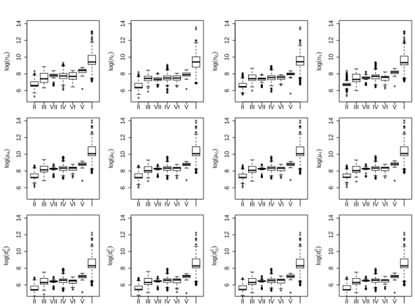
5.3 Box plots of summary statistics for genome sequences with Bal-timore Class labels. . . 73

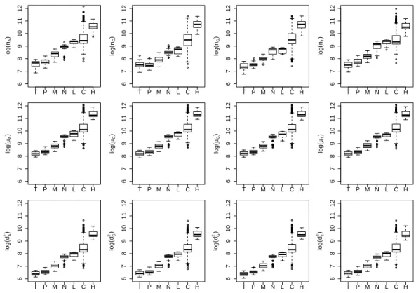
5.4 The same as Fig. 5.3 but for genome sequences with ICTV Or-der labels.. . . 74

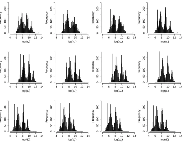
5.5 Histograms of genome sequence-related summary statistics for Baltimore Class-labelled viruses. . . 75

5.6 The same as Fig. 5.5 but for virus with ICTV Order labels. . . . 76

5.7 Histograms of mean nucleotide position normalised by genome length for viruses with Baltimore Class labels and ICTV Order labels. . . 76

5.8 Scatter plots between summary statistics for genome sequences. 77 5.9 t-SNE visualisation of sequences using NV and its derivatives coloured by taxonomic classes. . . 78

5.10 t-SNE visualisation of sequences using NV and its derivatives coloured by Length. . . 79

(13)

List of Figures 13 5.11 t-SNE visualisation of the sequences using 6-mer NV coloured

by taxonomic classes. . . 80

5.12 Box plots of the nucleotide content of virus genome sequences. . 81

5.13 Plots of overall nucleotide composition against genome length. . 82

5.14 Ternary plot of the nucleotide composition using three 2-letter alphabets (partition of the plot). . . 83

5.15 Ternary plot of the nucleotide composition using three 2-letter alphabets (Baltimore Classes). . . 84

5.16 Ternary plot of the nucleotide composition using three 2-letter alphabets (ICTV Orders). . . 85

5.17 Distribution of MAW in genome sequences. . . 86

5.18 The relationship between genome length and MAW. . . 87

5.19 Box plots of compression ratio achieved by general-purpose compression tools. . . 89

5.20 Box plots of compression ratio achieved by DNA-specific com-pression tools. . . 89

5.21 Histogram of compression ratio achieved by general-purpose compression tools. . . 90

5.22 Histogram of compression ratio achieved by DNA-specific com-pression tools. . . 90

6.1 Error bar plots of classification errors shown in Table 6.2. . . 95

6.2 Confusion matrix for the Baltimore Class experiment. . . 99

6.3 Confusion matrix for the ICTV Order experiment. . . 100

6.4 t-SNE visualisation of the distribution of difficulty levels of viruses. . . 102

7.1 Scatter plots of L1-SVM weights w learned from each pair of Baltimore Classes during a one-vs-one multi-class scheme. . . . 113

7.2 Scatter plots of L1-SVM weights w learned from each pair of ICTV Orders during a one-vs-one multi-class scheme. . . 113

(14)

8.1 Hierarchical structure of virus taxonomic classes. . . 134 8.2 Box plot of the class size at each level of the original and

modi-fied ICTV tree. . . 135 8.3 The class size at each level of the original and modified ICTV tree.136 8.4 Performance of SL and SSL in binary-class classification. . . 142

(15)

List of Tables

2.1 The non-satellite non-segmented virus genome sequences

la-belled by Baltimore Class and ICTV Order. . . 31

2.2 Membership of non-satellite non-segmented viruses in the Bal-timore Class and ICTV Order schemes. . . 32

2.3 Membership of non-satellite multi-segmented viruses in the Baltimore Class and ICTV Order schemes. . . 32

2.4 The non-satellite non-segmented virus genome sequences la-belled by hosts. . . 33

2.5 Entropy of virus classification for each taxonomic scheme. . . . 34

2.6 Labelling rate at each ICTV hierarchical level. . . 35

2.7 ICTV label assignment for non-satellite non-segmented viruses in the dataset. . . 36

3.1 Software packages and functions for the machine learning tech-niques used. . . 44

3.2 Confusion matrix for binary classification of classes labelled with +1 or -1. . . 53

3.3 Confusion matrix for multi-class classification of classes la-belled withC1, ...,Cn. . . 53

4.1 Genome sequence features based on nucleotide statistics. . . 58

4.2 Alphabets used to construct feature vectors.. . . 61

4.3 Dimensions of differentk-mer feature vectors. . . 61

(16)

5.1 Software packages and functions used for visualisation . . . 71

6.1 Range of parameter values used during cross-validation. . . 93

6.2 Classification error rates of different combinations of features and classifiers. . . 95

6.3 Number of viruses with different levels of difficulty. . . 101

6.4 Membership of level 3 viruses identified in Baltimore Class ex-periments. . . 102

6.5 Membership of level 3 viruses identified in ICTV Orders exper-iments. . . 103

6.6 Classification error rates of different classifiers. . . 104

6.7 Predicted classes for unlabelled viruses. . . 105

6.8 Prediction agreement between classifiers. . . 105

6.9 Error rates for virus host prediction.. . . 106

7.1 Range of parameter values used during cross-validation. . . 109

7.2 Classification error rate of different features and classifiers us-ing thek-mer NV of ACGT. . . 110

7.3 Classification error rate of different features and classifiers us-ing the concatenatedk-mer NV of ACGT. . . 112

7.4 Classification error rate of different features and classifiers us-ingk-mer counts of ACGT. . . 114

7.5 Classification error rate of different features and classifiers us-ingk-mer counts of SW. . . 115

7.6 Classification error rate of different features and classifiers us-ingk-mer counts of RY. . . 116

7.7 Classification error rate of different features and classifiers us-ingk-mer counts of MK.. . . 117

7.8 Classification error rate of different features and classifiers us-ing concatenatedk-mer counts of SW, RY and MK. . . 118

(17)

List of Tables 17 7.9 Classification error rate of different features and classifiers

us-ing RTD of ACGT. . . 119 7.10 Classification error rate of different features and classifiers

us-ing the concatenation of count and RTD of ACGT. . . 120 7.11 Classification error rate of different features and difference

measures using MAW. . . 122 7.12 Classification performance using features based on

compres-sion ratios of general-purpose comprescompres-sion tools. . . 123 7.13 Classification performance using features based on the

com-pression ratios of DNA specific comcom-pression tools. . . 124 7.14 The best performance achieved by each feature. . . 125 7.15 Membership of viruses whose Baltimore Class labels disagree

with the annotated labels. . . 126 7.16 Membership of viruses whose ICTV Order labels disagree with

the annotated labels. . . 127 7.17 Predicted classes for unlabelled viruses. . . 127 7.18 Confusion matrix of predicted Baltimore Classes for unlabelled

viruses. . . 128 7.19 Confusion matrix of predicted ICTV Orders for unlabelled

viruses. . . 128 7.20 Classification error rate of different features and classifiers

us-ing thek-mer NV of ACGT. . . 129 7.21 Classification error rate of different features and classifiers

us-ingk-mer counts of ACGT. . . 130 7.22 Classification error rate of Baltimore Class prediction for

multi-segmented viruses. . . 130

8.1 Summary statistics of the class sizes of the original and modified ICTV tree. . . 134 8.2 Classification performance of SVM and k-mer counts at

(18)

8.3 Classification performance of SL-based flat and hierarchical classifiers at individual ICTV taxonomic levels. . . 139 8.4 Classification performance of SL-based flat and hierarchical

classifiers measured using hierarchical loss. . . 139 8.5 Performance of SL and SSL in multi-class classification. . . 143 8.6 Classification performance of SSL-based flat and hierarchical

classifiers at individual ICTV taxonomic levels. . . 144 8.7 Classification performance of SSL-based flat and hierarchical

classifiers measured using hierarchical loss. . . 144 8.8 Number of classes and samples in each group. . . 145 8.9 Classification error rates for classes in each group. . . 146

(19)

19

List of Abbreviations

CV Cross-Validation

DT Decision Tree

FC Flat Classifier

GC Global hierarchical Classifier

ICTV International Committee on Taxonomy of Viruses

k-NN k-Nearest Neighbour classifier

k-NNG k-Nearest Neighbour Graph

LCL Local hierarchical Classifiers per Level

LCN Local hierarchical Classifiers per Node

LCPN Local hierarchical Classifiers per Parent Node

MAW Minimal Absent Word

MST Minimum Spanning Tree

MV Majority Vote

NCBI National Center for Biotechnology Information

NCD Normalised Compression Distance

NV Natural Vector

RBF Radial Basis Function

RF Random Forest

RTD Return Time Distribution

SL Supervised Learning

SSL Semi-Supervised Learning

SVM Support Vector Machine

t-SNE t-Distributed Stochastic Neighbour Embedding

(20)

Introduction

This chapter introduces the motivation for our work, the aims and contributions, and outlines the thesis.

1.1 Motivation

Virus taxonomy is the task of placing viruses into a taxonomic system, a scheme that groups organisms together on the basis of shared features such as evolutionary history, phenotypic characteristics, and biological properties [2].

Virus taxonomy has significant implications for both the scientific community and for practising clinicians. For the virologist, the classification of viruses pro-vides a better insight into their biological properties. The task is challenging since the question of whether viruses are a type of life is already a controversial topic, and the taxonomical criteria established in the cellular kingdoms of life (Eubacte-ria, Archaea, Protista, Fungi, Plantae and Animalia) do not generally apply to the acellular kingdom of viruses [3, 2, 4]. The task is important to the understanding of life because it unveils new principles of life processes and promotes new directions in science [5, 6, 7].

For clinicians, virus taxonomy provides a reliable basis for medically signif-icant differentiation, allowing for enhanced diagnostic procedures and epidemio-logical studies as well as facilitating the treatment and prevention of disease. For example, the introduction of diagnostic procedures based on nucleic acid sequences has increased the need for precise classification of viruses in accordance with their

(21)

1.1. Motivation 21 molecular characteristics [8]. The identification of virus hosts has practical impor-tance in the prevention of potentially large scale epidemics [9].

1.1.1 Virus taxonomic schemes

Virus taxonomic schemes evolve over time as virology progresses and technology develops. In the early days of virology when genome sequences were unavailable, viruses were classified and named after the host or location where they were first discovered. Such taxonomy is completely based on phenetic properties. Nowadays, host range is still an important property of a virus and is one of the criteria used for classification [2].

Modern taxonomy relies more heavily on the genetic properties of viruses. Currently, two main taxonomic systems are in use: the Baltimore scheme and the International Committee on Taxonomy of Viruses (ICTV) scheme. The Baltimore scheme [10] defines seven classes based on genome organisation and replication strategy, assigning a virus to Baltimore Class I, II, III, IV, VI, VI or VII according to its nucleic acid type (DNA or RNA), strandedness (single or double), genome polar-ity (positive-sense or negative-sense), and method of viral mRNA synthesis (reverse transcription or not). The ICTV scheme [2] defines a hierarchy based on multiple criteria, including the genome sequence and relationships to known viruses. A virus is assigned to a newly suggested or extant Order (most general), Family, Subfamily, Genus and Species (most specific) following proposals made by virologists. Viruses designated as the same Species have several properties in common but need not have a single common defining property. Those assigned to the same class at a higher (more general) level in the hierarchy share certain common properties from lower level classes.

1.1.2 The need for automated genome sequence-based

tech-niques

Manually classifying a virus can be a laborious task and involves a lengthy pro-cess. It is typically done case by case through proposals by experienced virolo-gists, who make significant efforts to understand the various biological properties

(22)

of certain virus groups [2]. With rapid advances in sequencing technology gen-erating large numbers of virus genome sequences at an ever increasing rate, these genome sequences are often the only information available for a virus in many real world situations [4]. Manual approaches to virus taxonomy are unable to handle this tsunami of data and to incorporate the newly identified viruses into existing systems in a timely and efficient manner. Thus, automated methods for classifying viruses given only the primary structure of virus genomes are needed to aid the work of taxonomists.

Given the rich evolutionary history of the virus kingdom, a taxonomy based only on genome sequences may not properly reflect their phylogenetic properties and thereby yield fewer biological insights [4, 3]. However, the overall effective-ness and efficiency of such methods make them useful tools for taxonomy-related tasks, and it is broadly agreed that the development of a robust framework for sequence-based virus taxonomy is indispensable to the comprehensive character-isation of viruses [11, 12, 13]. Moreover, at a recent ICTV workshop, experts reached a consensus that with appropriate quality control, viruses that are known only from metagenomic data should be incorporated into the official ICTV classifi-cation scheme [14].

1.1.3 Methods for sequence comparison

In order to perform genome sequence-based virus taxonomy, methods for sequence comparison are required to establish the relationship between different viruses. In general, genome sequence-based taxonomy can be divided into two types: alignment-based and alignment-free methods.

Alignment-based methodsAlignment-based methods are the traditional approach to sequence comparison, and classify viruses based on the degree to which their genome sequences can be matched. These methods first identify conservative re-gions in the genome sequences, align them through insertion, deletion and mutation, and then derive distance measures between the genomes using alignment scores.

Numerous such techniques exist, mainly differing in the way the sequences are aligned and/or the scores derived (see [15, 16] for detailed reviews). For example,

(23)

1.1. Motivation 23 alignment can be performed between every two sequences [17, 18, 19] or between multiple ones simultaneously [20, 21, 22]; alignment can be performed based only on certain local structures of sequences [23, 24, 18] or on the global structure as a whole [25, 26, 27]. A wide range of scoring systems have also been proposed, such as the substitution scoring matrices PAM [28] and BLOSUM [29].

These methods perform well for relatively small datasets consisting of similar sequences, however can suffer from both computational and fundamental limita-tions on larger datasets with diverse sequences. In terms of computational load, optimal sequence alignment can be infeasible for the large corpora of sequences produced by next generation sequencing technologies [30, 31]. Alignment-based methods (e.g. [23, 21]) typically require time and space complexity on the order of

O(L2), whereLis the average length of the sequences. More efficient methods (e.g.

[32, 33]) have been developed for specialised purposes, but typically assume spe-cific properties for the sequences being aligned. In terms of virological fundamen-tals, the evolutionary assumptions guiding the alignment and scoring procedures may not reflect the phylogeny, tending to overemphasize the importance of sequence similarity while overlooking the importance of functional similarity [34, 35]. In ad-dition, the scoring methods assume linearity of the evolutionary procedure, which, in fact, takes place at different scales simultaneously [36]. Moreover, due to the lack of a feature representation, they can only be combined with distance-based classi-fiers, which restrict the application of potentially more sophisticated and powerful machine learning techniques.

Alignment-free methodsIn contrast, alignment-free methods – the focus of this thesis, classify viruses based on the degree to which the features of different se-quences are similar. Instead of aligning sese-quences or deriving similarity scores, they first map a virus genome sequence to a point in feature space, where the dis-tance between features reflects the disdis-tance between the original sequences, then classify the virus in this space.

Alignment-free methods were initiated by [37]. Recent representations and approaches include using the statistics of nucleotide occurrence and positional

(24)

in-formation [38, 39], count of k-mers [40], Kolmogorov complexity of sequences [41], absent words [42, 43], matrix invariants [44], genomic signal processing [45], curves [46] and images [47].

In relying solely on the analysis of the genome sequence, alignment-free meth-ods suffer from the same drawbacks as alignment-based methmeth-ods, lacking biological insights into the functionalities of their viruses. However, the former improve upon the latter in several aspects. Firstly, since no alignment is needed, the associated bi-ological knowledge required to inform the alignment process is not required, which can be an advantage in situations where only the sequence is known. Secondly, they can cope with highly diverse sequences where reliable alignment is impossible [11]. Thirdly, they can handle large data sets more efficiently as all sequences are represented in a fixed format as points in a feature space. Furthermore, the usage of features allows for the application of a wider range of machine learning techniques,

such as the k-NN classifier [38, 48], association rule-based classifier [49], SVM

[50] and artificial neural networks [51].

An earlier work [52] shows that alignment-free methods using nucleotide statistics perform well for diverse virus genome sequences (above Genus level) but tend to become less accurate for similar ones (Genus and Species levels). However, later studies [48, 40] show that with more sophisticated features, alignment-free methods perform no worse than alignment-based ones even at Genus and Species levels. A recent work has proposed a strategy that exploits the complementary na-ture of alignment-based and alignment-free methods [53]. The classification of se-quences is performed by using a combined sequence similarity score (CSSS) that is calculated based on the weighted contribution of the scores of each method, where the weights reflect the discriminatory ability of individual measures in the training set. Scores combined from 3 alignment-free and 2 alignment-based methods show good performance in biological sequences.

(25)

1.2. Aims and contributions 25

1.2 Aims and contributions

The goal of this thesis is to advance automated virus taxonomy methods using only the primary structure of virus genomes, with the ultimate aim of complementing traditional manual approaches. We focus on alignment-free methods for sequence comparison, studying the performance of different features for genome sequences and machine learning techniques in the task of virus taxonomy.

Our aims are as follows. First, we will asses the extent to which information provided by genome sequences can be used to distinguish viruses from different tax-onomic classes. Next, we will investigate the predictive powers of different feature representations of genome sequences and classifiers in the task of virus taxonomy. Finally, we will devise classification strategies that outperform the current state of the art.

Our contributions are as follows. First, we conduct a thorough analysis of the NCBI reference genome sequence dataset that is frequently used by virolo-gists, exceeding previous studies in scale and depth (Chapter 5). We analyse sta-tistical properties of the nucleotide composition of genome sequences for all cur-rently discovered virus species, which provides insights into the efficacy of genome sequence-based taxonomy. We also analyse the predictive powers of different fea-ture representations for genomes based on their statistical properties. In addition, we apply visualisation techniques to display all the sequences in the dataset in two-dimensional space. Second, we conduct a systematic study to compare and contrast the predictive powers of various combinations of features and classifiers in the task of virus taxonomy, extending previous studies with a wider range of techniques from simple approaches to sophisticated ones (Chapter 6 and 7). With optimised experimental factors, the best combinations outperform the current state of the art. Using the best methods identified in our study, we make predictions for currently unlabelled sequences. Third, we are the first to explicitly incorporate hierarchical information and apply SSL-based hierarchical classifiers to the dataset in predict-ing the ICTV classes (Chapter 8). The SSL-based hierarchical methods outperform SL-based ones, which outperform non-hierarchical ones.

(26)

1.3 Thesis outline

The remainder of the thesis is organised as follows.

In Chapter 2, we describe the virus genome sequence dataset and taxonomic scheme used in our study, as well as presenting the summary statistics of the dataset. In Chapters 3 and 4, we review machine learning techniques for sequence clas-sification and feature representations for genome sequences. In Chapter 3, we re-view the machine learning techniques used in our study. We start by categorising learning techniques, comparing and contrasting different approaches. We then re-view the classifiers used in our study, including k-NN, RF, SVM, and Graph-based SSL. Following this, we review hierarchical classifiers, including their character-isations, approaches, relationships with each other as well as their bioinformatics applications. Finally, we discuss performance measures used for non-hierarchical and hierarchical classification.

In Chapter 4, we review the alignment-free feature representations used in our study. We first describe nucleotide-based features, including NV and its derivatives.

We then describe word-based features, which includek-mer count,k-mer NV, RTD

and MAW. In addition, we describe compression-based features derived from both general and DNA-specific compression tools.

Chapters 5 to 8 contain our key observations, results and contributions. In Chapter 5, we perform a thorough exploratory analysis of the the entire virus genome sequence dataset, exceeding prior work in scale and depth. The analysis aims to better understand the properties of the dataset, as well as informing hy-pothesis formulation and experimental design in later chapters. We explore differ-ent properties of composition- and location-related nucleotide statistics, word and compression-based features, as well as the dataset as a whole using various visuali-sation techniques, including ternary plots and t-SNE visualivisuali-sations.

In Chapter 6, we extend previous work by performing a systematic study of the classification performance of the NV and its derivatives. We study the pre-dictive power of NV and its components combined with various machine learning techniques, from the simple 1-NN and k-NN classifiers used in previous works, to

(27)

1.3. Thesis outline 27 more advanced SVM and RF classifiers that have not been explored before. Using the best experimental settings, we identify viruses that are consistently misclassi-fied and predict labels for currently unlabelled sequences. We also investigate the performance in predicting virus hosts.

In Chapter 7, we extend the nucleotide-based features used in Chapter 6 to more sophisticated word and compression-based features. We perform the first sys-tematic study of the classification performance of a wide range of features and clas-sifiers. As in Chapter 6, using the best experimental settings, we identify viruses that are consistently misclassified and predict labels for currently unlabelled sequences. We also investigate the performance in predicting virus hosts and taxonomic classes for multi-segmented viruses.

In Chapter 8, we design hierarchical classification approaches based on the best non-hierarchical classifier identified in Chapter 7 to classify viruses into hier-archical ICTV taxonomic classes. We are the first to explicitly incorporate ICTV hierarchical information into classification, and also the first to apply SSL-based hierarchical classifiers to the classification of ICTV taxonomic classes.

(28)

Virus genome sequence datasets

This chapter describes the types of public virus genome sequence datasets and pro-vides an overview of the dataset used in our study. We use a genome sequence dataset provided by the National Center for Biotechnology Information (NCBI), which is part of the United States National Library of Medicine, a branch of the National Institutes of Health. The NCBI houses a series of databases relevant to biotechnology and biomedicine and is an important resource for bioinformatics tools and services.

2.1 Types of datasets

The NCBI provides two types of virus genome sequence datasets: a reference se-quence dataset that contains a single record for each model virus species, and a comprehensive dataset that contains all publicly available records for individual viruses. They are available through the Reference Sequence database (RefSeq) [54] and the GenBank database [55] respectively.

2.1.1 RefSeq

The RefSeq database is an open access, annotated and curated collection of pub-licly available nucleotide sequences and their protein products. The collection aims to provide, for each model species, a complete set of non-redundant, extensively cross-linked, and richly annotated nucleic acid and protein records. Each record represents a synthesis of the primary information of a species that was generated and submitted by different research groups. The database is curated on an ongoing

(29)

2.2. Summary of the experimental dataset 29 basis by collaborating groups and NCBI staff. Sequence records are presented in a standard format and subjected to computational validation. The collection estab-lishes a useful baseline for integrating diverse data types.

2.1.2 GenBank

The GenBank database is also an open access collection of nucleotide sequences and protein products. In contrast to the RefSeq database, its aim is to provide a com-prehensive collection of all original sequences. Each record represents the primary information of an individual virus submitted by a group, by whom the copyright is retained. The originality and quality of the sequences are checked by the NCBI staff, but the sequences themselves are not curated. The collection establishes a comprehensive archive for discovered and approved sequences.

2.2 Summary of the experimental dataset

Since the theme of the thesis is to investigate the effectiveness of genome sequence-based techniques in the task of virus taxonomy, we are interested in genome se-quences representative of virus species rather than individuals. Therefore, we use the RefSeq dataset as it contains high quality and complete model genomes for each virus species.

The RefSeq dataset was retrieved from the “Viruses” directory of the NCBI

FTP site on 18th September 2015 [56]. Each of the 4,420 downloaded

fold-ers contains the complete genome sequence and annotation for a virus species. A virus genome can consist of a single or multiple nucleotide segments. The dataset contains 3,910 non-segmented viruses (of which 211 are satellites)

and 510 multi-segmented viruses (of which 6 are satellites). We remove all

satellites from the dataset, leaving genome sequence data for the 3,699 non-satellite non-segmented viruses and 504 non-non-satellite multi-segmented viruses

for later experiments. We focus our study on non-segmented viruses since

the number of multi-segmented viruses is small. Virus host labels are not

available from the “Viruses” directory, which we downloaded separately from http://www.ncbi.nlm.nih.gov/genome/browse/.

(30)

2.3 Taxonomic schemes

We consider three different taxonomic schemes with decreasing levels of depen-dence on genome sequences: ICTV Orders, Baltimore Classes and virus hosts. The Baltimore scheme classifies viruses into 7 non-hierarchical classes whereas the ICTV scheme defines a hierarchy starting at 7 Orders and progressing through 77 Families, 19 Subfamilies and finally 371 Genera. The viruses are also assigned 14 different host labels, which we reduce to 4 non-hierarchical classes Archaea, Bacteria, Eucaryote 1 and Eucaryote 2.

2.3.1 Non-hierarchical classes

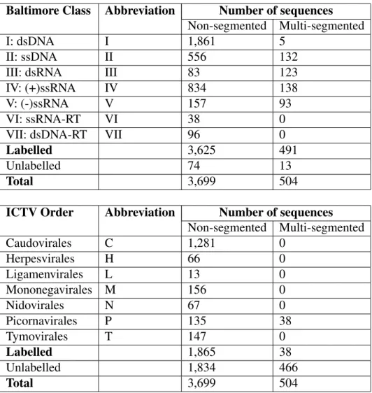
Table 2.1 breaks down the 3,699 non-segmented and the 504 multi-segmented viruses investigated by Baltimore Class and ICTV Order. Table 2.2 and 2.3 show their membership in the two schemes. They reveal that an ICTV Order is a subgroup of a Baltimore Class, i.e. each Baltimore Class contains multiple ICTV Orders but each ICTV Order belongs to only one Baltimore Class. Table 2.4 breaks down the 3,699 non-segmented viruses by their hosts. The fourteen host labels are divided into four groups in order to balance the class sizes and avoid overlaps in constitut-ing hosts.

In our non-hierarchical classification experiments of non-segmented viruses, we classify a virus genome sequence into one of the 7 Baltimore Classes, one of the 7 ICTV Orders or one of the 4 host groups. Due to the small number of labels available for multi-segmented viruses, our experiments classify each of them into one of the 4 Baltimore Classes II, III, IV or V. Table 2.5 summarizes the entropy of the classification problem for each taxonomic scheme.

(31)

2.3. Taxonomic schemes 31

Baltimore Class Abbreviation Number of sequences

Non-segmented Multi-segmented

I: dsDNA I 1,861 5

II: ssDNA II 556 132

III: dsRNA III 83 123

IV: (+)ssRNA IV 834 138

V: (-)ssRNA V 157 93

VI: ssRNA-RT VI 38 0

VII: dsDNA-RT VII 96 0

Labelled 3,625 491

Unlabelled 74 13

Total 3,699 504

ICTV Order Abbreviation Number of sequences

Non-segmented Multi-segmented Caudovirales C 1,281 0 Herpesvirales H 66 0 Ligamenvirales L 13 0 Mononegavirales M 156 0 Nidovirales N 67 0 Picornavirales P 135 38 Tymovirales T 147 0 Labelled 1,865 38 Unlabelled 1,834 466 Total 3,699 504

Table 2.1: The non-satellite non-segmented virus genome sequences labelled by Balti-more Class and ICTV Order.

For each taxonomic scheme, the complete name of a Baltimore Class or ICTV Order, its abbreviation, and the number of sequences assigned that taxonomic label are listed. The row “Labelled” shows the number of sequences assigned any one of the seven labels. “Unlabelled” is the number of sequences with no label. “Total” is the number of labelled and unlabelled sequences. For the Baltimore scheme, “ds” denotes double-stranded, “ss” single-stranded, “(+)” positive-sense, “(-)”

(32)

I II III IV V VI VII Unlabelled C 1281 0 0 0 0 0 0 0 H 66 0 0 0 0 0 0 0 L 13 0 0 0 0 0 0 0 M 0 0 0 0 156 0 0 0 N 0 0 0 67 0 0 0 0 P 0 0 0 135 0 0 0 0 T 0 0 0 147 0 0 0 0 Unlabelled 501 556 83 485 1 38 96 74

Table 2.2: Membership of non-satellite non-segmented viruses in the Baltimore Class and ICTV Order schemes.

For each Baltimore Class (column), the number of viruses assigned that taxonomic label and an ICTV Order (row) or no additional label (row “Unlabelled”) is shown. For example, the entry corresponding to the row “H” and column “I” means there are 66 viruses from Baltimore Class “I” and ICTV Order “H”. The table shows abbreviations of class names, see Table 2.1 for the full names.

I II III IV V Unlabelled

P 0 0 0 38 0 0

Unlabelled 5 132 123 100 93 13

Table 2.3: Membership of non-satellite multi-segmented viruses in the Baltimore Class and ICTV Order schemes.

The same as Table 2.2 but for non-satellite multi-segmented viruses. Missing Baltimore Classes and ICTV Orders correspond to columns and rows consisting of zeros only.

(33)

Host group Abbreviation Hosts Number of Total

sequences Archaea A Archaea 63 63 Bacteria B Bacteria 1,421 1,421 Eucaryote 1 E1 Algae 40 137 Fungi 67 Protozoa 30 Eucaryote 2 E2 Invertebrates 234 2,023 Invertebrates, plants 38 Invertebrates, vertebrates 4 Plants 726 Vertebrates 736 Vertebrates, human 215 Vertebrates, invertebrates 23

Vertebrates, invertebrates, human 47

Subtotal 3,644

Environment 43

Labelled 3,687

Unlabelled 12

Total 3,699

Table 2.4: The non-satellite non-segmented virus genome sequences labelled by hosts.

The fourteen virus host labels obtained from the dataset, excluding Environment, are divided into four groups: Archaea (A), Bacteria (B), Eucaryote 1 (E1) and Eucaryote 2 (E2). For each host group, its name, abbreviation, constituent hosts, the number of sequences assigned to that host, and the total number in the group are shown. Row “Subtotal” is the number of sequences used in our experiments. “Environment” is the number of sequences assigned Environment as host, which are excluded from our experiments. “Labelled” is the number of sequences assigned any one of the four labels. “Unlabelled” is the number of sequences with no host labels. “Total” is the number of all the sequences listed in the table.

(34)

Segment type Taxonomic scheme Possible classes Entropy

Non-segmented Baltimore Class I, II, III, IV, V, VI, VII 0.252

Non-segmented ICTV Order C, H, L, M, N, P, T 0.432

Non-segmented Host group A, B, E1, E2 0.111

Multi-segmented Baltimore Class II, III, IV, V 0.117

Table 2.5: Entropy of virus classification for each taxonomic scheme.

The table shows virus segment type, taxonomic scheme used, possible classes in the classification problem and entropy. Entropy is computed as

H(X) =−∑c_i=1piln(pi), wherecis the number of possible classes in the

classification problem,lnis the natural log, and p_iis the probability of a virus

coming from classi, which we assign to the inverse of the number of total labelled

(35)

2.3.2 Hierarchical classes

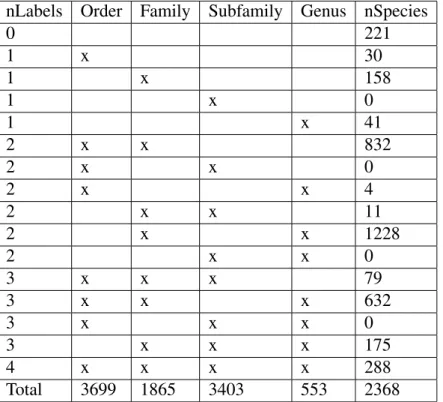
The ICTV scheme organizes the classes as a hierarchical taxonomic tree, and from the highest to the deepest levels are Order, Family, Subfamily, Genus and Species respectively. The tree is balanced where every leaf node is at exactly the same depth. Table 2.6 shows the labelling rate at each ICTV hierarchical level for the 3,699 non-satellite non-segmented viruses in the dataset. Table 2.7 summarises the labelling conditions for individual sequences of model species. Among them, 221 species are not assigned to any high level classes and only 288 have labels at all levels. Our hierarchical classification experiments aim to assign the genome sequence of each model Species in the dataset into the Order, Family, Subfamily and Genus that it belongs to.

Taxonomic level Number of classes Number of labelled genomes Labelling rate

Order 7 1865 0.504

Family 77 3403 0.920

Subfamily 19 553 0.149

Genus 371 2368 0.640

Species 3699 3699 1

Table 2.6: Labelling rate at each ICTV hierarchical level.

The table shows the number of classes, number of labelled genomes and labelling rate (the proportion of viruses having a label at the given level) at each ICTV taxonomic level.

(36)

nLabels Order Family Subfamily Genus nSpecies 0 221 1 x 30 1 x 158 1 x 0 1 x 41 2 x x 832 2 x x 0 2 x x 4 2 x x 11 2 x x 1228 2 x x 0 3 x x x 79 3 x x x 632 3 x x x 0 3 x x x 175 4 x x x x 288 Total 3699 1865 3403 553 2368

Table 2.7: ICTV label assignment for non-satellite non-segmented viruses in the dataset.

The column “nLabels” shows the number of higher level labels a genome sequence of a model species has. The columns “Order”, “Family”, “Subfamily” and “Genus” show the levels of the present labels. The corresponding level is marked with an “x” if a label is present. The last column “nSpecies” shows the number of species with the given “nLabels”. The last row “Total” shows the total number of viruses in the dataset, as well as the total number of those labelled at corresponding levels.

(37)

Chapter 3

Machine learning techniques

Machine learning techniques are computational algorithms that are able to extract rules from training data (learning) and apply these to testing data (prediction) with-out being explicitly programmed [57, 58, 59]. Among other uses, they can automate manual tasks to aid human experts in the analysis of large and complex data sets. In genomics, machine learning is perhaps most useful for the interpretation of large genomic data sets and has been used to annotate a wide variety of genomic sequence elements [60].

This chapter reviews the categories of machine learning techniques, the non-hierarchical and non-hierarchical classifiers and performance measures we use in our study.

3.1 Categories of machine learning techniques

Machine learning techniques can be categorized in a number of different ways. For instance, depending on whether each training sample is assigned a class label, they can be divided into supervised, unsupervised and semi-supervised methods. They can also be divided depending on whether distance matrices or feature vectors are required as the input, or they can be divided into distance-based and feature-based methods, or depending on whether the classes have a hierarchical relationship between each other, divided into non-hierarchical and hierarchical methods.

(38)

3.1.1 Supervised vs unsupervised vs semi-supervised

Machine learning techniques can be divided into three main classes based on the presence of labels when building models: supervised learning (SL), where la-belling information of known data guides the learning process; unsupervised learn-ing (USL), where rules are learned by the intrinsic properties of the data without the aid of labelling information; and semi-supervised learning (SSL), which combines labelled and unlabelled data during learning and prediction. When applied to virus taxonomy, SL techniques (such as classification) can be used to predict the taxa labels of a new virus. On the other hand, USL techniques (such as clustering) can be used to explore natural groups of viruses and construct phylogenetic trees. The third type, SSL techniques, can be used to improve classification or clustering in the situation where taxa labels are available for a small number of samples but are missing for the others. This thesis focuses on SL and SSL for classification.

3.1.2 Distance-based vs feature-based

Machine learning methods can be divided into three types based on the mechanisms they use to operate on distance measures and features. The first are distance-based methods, such as k-nearest neighbours (k-NN) and k-means. They do not require feature representations of the samples as long as their pairwise distance can be ob-tained. These methods take the distance matrix computed from all the samples as input and group nearby ones together. The second type are feature-based methods, such as Decision Trees (DT) and Random Forests (RF). In contrast to distance-based methods, feature representations of the original data are compulsory. These methods take the feature of a sample as input and assign labels by examining the discriminative power of the individual variables constituting each feature. The third type combine the above two, including Support Vector Machines (SVM) and other kernel methods. They require both a specific distance measure definition and fea-ture representation. Kernel methods take feafea-tures as input and implicitly transform them into a high-dimensional space through a kernel function, which plays a similar role to a distance measure.

(39)

3.2. Non-hierarchical classifiers 39 and alignment-free methods for sequence analysis: the lack of features restricts alignment-based methods to distance-based methods only, whereas the availability of features allows a wide range of classifiers to be combined with alignment-free methods. A brief discussion about distance and feature-based methods for sequence classification can be found in [61].

3.1.3 Non-hierarchical vs hierarchical

Machine learning methods can also be divided into non-hierarchical and hierar-chical approaches depending on whether the different classes of samples have a hierarchical relationship with each other. Most machine learning techniques are not originally designed to address hierarchical relationships explicitly and they typ-ically assume no hierarchical relationship between different classes. Hierarchical approaches are usually developed by incorporating hierarchical information into their non-hierarchical counterparts, which we call “base classifiers” in the context of hierarchical classification.

3.2 Non-hierarchical classifiers

We use three types of classifiers in our non-hierarchical classification experiments, k-NN, RF and SVM, representing distance-based methods, feature-based methods and those combining the two.

3.2.1 k-Nearest Neighbour (k-NN)

k-NN [62] is a classifier previously used in similar studies [52, 48]. To predict the label of a new virus genome sequence, it first computes the distance between the feature vector of the given sequence and that of all others in the training set, then makes a prediction using the majority vote of labels of the k-nearest neighbours

(sequences having the closest distance to the given one), wherekis a parameter of

the model. This is implemented by the functionknn[63] (Table 3.1).

3.2.2 Random Forest (RF)

RF [64] is an ensemble method consisting of a collection of Decision Trees. During training, a multitude of uncorrelated DT are constructed, with each tree built using

(40)

a random subset of virus genome sequences in the training set. To grow a tree, a random subset of feature variables are selected as candidates for node splitting, and the one that maximises a certain measure of information gain is used. The tree is then grown by repeatedly splitting nodes until termination conditions are met. To predict the label of a new sequence, each tree casts a unit vote for the predicted class and the one with the majority votes is the final output of the RF.

FunctionrandomForest[65] (Table 3.1) is an interface to the program by

Breiman and Cutler described in [64]. This builds a tree using two-thirds of the samples in the training set drawn randomly with replacement, splits each node of a tree using Gini impurity as the measure, then grows the tree using a CART (Clas-sification and Regression Tree) methodology [66] until all samples in a node are from the same class. The trees grown are not pruned. The function has two tunable

parameters. One isntree, the number of trees in the forest and another ismtry, the

number of variables randomly sampled for splitting a node. According to [64], the influence of the parameters are found to be small and a wide range of values tend to give optimal results.

3.2.3 Support Vector Machine (SVM)

The SVM [67, 68, 69] is a binary classifier that aims to find a separator that best sep-arates samples from different classes. The optimization goal is to find a hyperplane that maximises the margin – the distance of the samples closest to the hyperplane. Given training samples(xi,yi),i=1, ...,m, wherexi∈Rd is a feature vector of

di-mensiond and y_i∈ {−1,1}is the label of the i-th sample, the primal form of the

classical soft-margin problem is formulated as:

min w,b 1 2||w|| 2 2+C m

∑

i=1 εi, (3.1) s.t. yi(wTxi+b)≥1−εi, (3.2) εi≥0,i=1, ...,m. (3.3)

(41)

3.2. Non-hierarchical classifiers 41

A new samplexis classified assign(wˆTx+bˆ), where ˆwis the optimised parameter

vector and ˆb=y_j−wˆTxj. The dual form of the optimisation problem is

max αi −1 2 m

∑

i,j=1 αiαjyiyjxTi xj+

_∑

i αi, (3.4) s.t.

_∑

i yiαi=0, (3.5) 0≤αi≤C,i=1, ...,m. (3.6)

A new samplex is classified assign(∑m_i₌₁αˆiyixTi x+bˆ), where ˆαi is the optimised

parameter and ˆb=yj−∑m_i=1αˆiyixT_i x.

The benefit of the dual form is that a feature map φ(.) can be introduced to

enhance the separability of the data points. This is done by replacing the

origi-nal feature vector xi with φ(xi) and the corresponding similarity measure can be

computed using a kernel function K(xi,xj) =<φ(xi),φ(xj)>. Then the above

formulation becomes max αi − 1 2 m

∑

i,j=1 αiαjyiyjK(xi,xj) +

∑

i αi, (3.7) s.t.

_∑

i y_iαi=0, (3.8) 0≤αi≤C,i=1, ...,m. (3.9)

A new samplexis classified as sign(∑mi=1αˆiyiK(xi,x) +bˆ), where ˆαi are the

opti-mised parameters and ˆb=y_j−∑m_i₌₁αˆiyiK(xi,xj).

The role of a kernel function is to map the training samples to a high-dimensional space, where the data can be linearly separated by the hyperplane. The choice of kernel function determines the type of space the data points are

mapped to. The inner product between the original feature vector xT_i xj can be

considered as a linear kernel, and we denote the corresponding classifier Linear-SVM. Since the linear kernel has no parameters, the optimisation of Linear-SVM

is controlled by a single slack parameterC, which “softens” the constraints to

(42)

function is a radial kernel function [71] (Radial-SVM), where the optimisation is

controlled by two parameters. The first parameterCis the same as that in the linear

kernel function. The second parameterγ is the inverse “width” of the radial kernel

function, K(xi,xj) =exp(−γ||xi−xj||2), wherexi andxj are two feature vectors.

Functionsvmimplements Linear-SVM and Radial-SVM, which is an interface to

libsvm[72]. (Table 3.1).

One variation of the standard SVM can be derived by replacing the L2-norm regularizer in the objective function with an L1-norm regularizer [73] (L1-SVM). The optimisation problem can be formulated as

min w,b m

∑

i=1 max(0,1−yi(wTxi+b)), (3.10) s.t. ||w||1≤λ. (3.11)

This produces sparse solutions where only a certain proportion of the feature vari-ables are associated with non-zero weights and hence used to form the optimal

hyperplane. This proportion is controlled by the parameterλ, where a smaller λ

leads to fewer non-zero weights. Function svm.fsimplements L1-SVM (Table

3.1).

As the SVM was originally designed for binary classification, the package we use solves multi-class problems using a one-vs-one scheme. It first trains a binary classifier for each pair of candidate classes, voting for one of the two. The final prediction is obtained by taking the majority vote of the binary classifiers.

3.2.4 Graph-based semi-supervised learning (SSL)

Graph-based SSL [74, 75, 76] is a semi-supervised learning technique based on the graphical structure of the data.

Given a dataset X = {x1, ...,xl,xl+1, ...,xn} with n samples, of which only

l<<nare labelled, i.e. eachx_i,i=1, ...,lhas a labely_i∈ {−1,1}, but the remaining

i=l+1, ...,nare unlabelled, a graph can be constructed using thensamples, where

each vertex represents a sample and the edge weight w_{i j} betweenx_i andx_j

(43)

3.2. Non-hierarchical classifiers 43 degree of similarity between the labels of the two vertices. One of the heuristics used to specify edge weights is to construct a k-nearest neighbour graph (k-NNG), where each vertex defines its k-nearest neighbour vertices by Euclidean distance.

Two vertices are connected if one is among the other’s k-nearest neighbours. Ifxi

and x_j are connected, the edge weight w_{i j} is either the constant 1, in which case

the graph is said to have binary edge weights or be unweighted, or a function of the

distance such as the Radial Basis Function (RBF)w_{i j} =exp(−||xi−xj||2

2σ2 ). If xiand

xjare not connected,wi j is assigned zero. Empirically, k-NNG with small k tend to

perform well [76].

Once the graph is constructed, learning involves assigning labels to unlabelled

vertices xi,i=l+1, ...,n such that disagreement of labels between neighbouring

vertices is minimised while satisfying the constraint that the assignment forxi,i=

1, ...,lmatch their true labelsy_i. This is done by solving the following optimisation problem min f∈R n

∑

i,j=1 w_{i j}(f_i−f_j)2, (3.12) s.t. f_i=y_i,i=1, ...,l, (3.13)

where sign(fi) will be the predicted label for xi. The matrix form of the above

problem is

min

f∈Rn f

0_L_f, _(3.14)

s.t. fl=yl, (3.15)

where f = [fl,fu]0, sign(fl) contains the predicted labels for labelled samples,

sign(f_u) contains the predicted labels for unlabelled samples,y_l = [y₁, ...,y_l]0

con-tains the true labels for the labelled samples,L=D−W is the Laplacian matrix,D

is a diagonal matrix withD_ii=∑n_j₌₁wi j andW = (wi j)n×n is the adjacency matrix

(44)

finding the stationary point of the objective function, which is

fu=−L−uu1Lulyl, (3.16)

where Luu andLul are sub-matrices of Lwhen partitioned into labelled and

unla-belled components L=   L_ll L_ul L_lu Luu  . (3.17)

Normalisation of the algorithm can be achieved by ensuring the degree of each

ver-tex is unity, which is done by replacing the Laplacian matrixLwith the normalised

versionL=I−D−1/2W D−1/2, whereIis the identity matrix. Similarly to the SVM,

the technique was originally designed for binary classification. Here, we extend it to multi-class problems with the same one-vs-one scheme that is used for SVM, where a binary classifier is trained for each pair of classes and the final prediction is the majority vote from all participating binary classes. SSL is implemented in-house (Table 3.1).

3.2.5 Software

Here, we list the software packages and functions for the machine learning tech-niques used in our experiments.

Algorithm Function name R 3.1.3 package [77]

k-NN knn class [63]

RF randomForest randomForest [65]

Linear-/Radial-SVM svm e1071 [78]

L1-SVM svm.fs penalizedSVM [79]

Graph-based SSL graphSSL VirusTaxonomy [80]

Table 3.1: Software packages and functions for the machine learning techniques used.

3.3 Hierarchical classification

Non-hierarchical classification aims to predict the class for a given sample, whereas hierarchical classification aims to predict a set of hierarchically structured classes for each sample. Comprehensive reviews of hierarchical classification can be found

(45)

3.3. Hierarchical classification 45 in [81, 82].

3.3.1 Characterisations

In a hierarchical classification problem, the label of a sample is a vector, where each element is a class at a specific level of the hierarchy that the sample belongs to, and different elements are related through a hierarchical structure. A hierarchical clas-sification problem can be characterised by three aspects. The first is the graph of the hierarchical structure. Possible variations include the tree or directed acyclic graph (DAG) structure, which differs in the number of parents a class can have. The second is the number of labels a sample can have at one level. Possible variations are single or multiple label classification. The third is the labelling depth of a sam-ple. Possible variations include mandatory or non-mandatory leaf node prediction, which differ in whether it is mandatory to label each sample with the leaf node classes. The hierarchical classification problem studied in this thesis involves tree, single label and mandatory leaf node prediction.

Hierarchical classifiers can be categorized into three types depending on how the hierarchical information is used: the flat classifier (bottom-up) approach, local classifier (top-down) approach and global classifier (big-bang) approach. The flat approach is the simplest solution to hierarchical classification, and is essentially a regular multi-class classifier at the deepest level plus a post-processing step that fills in the higher level labels. In contrast, the local and the global approaches ex-plicitly incorporate the class hierarchy into the classification. The local approach is an ensemble method that combines multi-class non-hierarchical classifiers (base classifiers), whereas the global approach involves formulating a single optimisa-tion problem taking into account the class hierarchy. In the next few secoptimisa-tions, we will explain in detail the procedures for applying flat, local and global classifiers to classify samples into hierarchical classes.

3.3.2 Flat classifier

The flat classification approach, which is the simplest way to address hierarchical classification problems, consists of predicting classes only at the leaf nodes and

(46)

then filling in higher level labels during post-processing. For instance, to build a flat classifier for the class structure shown in Fig. 3.1, it trains one multi-class classifier that distinguishes among the four leaf nodes 1.1, 1.2, 2.1, and 2.2. During testing, it classifies a test sample into one of the leaf nodes. Since the structure is a tree, there is only one unique path from a given leaf to the root. Hence once the leaf class is known, its ancestors are by definition also obtained..

The learning and prediction stages of this approach are essentially the same as for non-hierarchical classifiers. However, it provides an indirect solution to hier-archical classification problems because when a leaf class is assigned to a sample, all its ancestor classes are also implicitly assigned as the class hierarchy is known a priori. This very simple approach has the disadvantage of having to build a classifier to discriminate among a large number of classes (all leaf classes) with a small num-ber of samples per class, without exploiting information about parent-child class relationships present in the class hierarchy.

Figure 3.1: Class structure used to illustrate the procedures of applying different hi-erarchical classifiers.

The graph is a tree with seven nodes, each representing a class and the edges con-necting them represent the parent-child relationship. The node R is the root class, sitting at the highest level of the hierarchy and is the ancestor of all other classes. Node 1 and 2 at the next level are two child classes of the root. Leaf nodes 1.1, 1.2, 2.1 and 2.2 are at the bottom of the hierarchy and are children of class 1 and class 2. The goal of the hierarchical classifier is to predict, for a sample, the set of classes forming a complete path from the root to the leaf.

(47)

3.3. Hierarchical classification 47

3.3.3 Local classifier

The local classifier approach incorporates class hierarchy information by combining multiple base classifiers. Different methods differ in how they use local information and how they build their classifiers around it. Specifically, there are three standard ways of using the local information [81]. The first is one Local Classifier per Node (LCN), which trains base classifiers to distinguish a certain class among all the oth-ers. The second is one local classifier per level (LCL), which trains base classifiers to distinguish a certain class among all the others in the same hierarchical level. The third is one Local Classifier per Parent node (LCPN), which trains base classifiers to distinguish a certain class among all its siblings. We will illustrate the procedures for applying the three local classifiers using the class structure shown in Fig. 3.1.

LCN.When applying the LCN approach, six binary classifiers will be trained, one

per node excluding the root: classifier 1 distinguishes node 1 from the rest, classifier 2 distinguishes node 2 from the rest, and so forth. During testing, a test sample would be classified into one of the two classes by each binary classifier, and the final predicted class path obtained after a post-processing step to correct any class inconsistency (see section “Inconsistency correction for LCN and LCL”).

LCL.When applying the LCL approach, two multi-class classifiers will be trained,

one per level excluding the root level: classifier 1 for nodes 1 and 2 at level 1, classifier 2 for nodes 1.1, 1.2, 2.1 and 2.2 at level 2. If the base classifier is orig-inally designed for binary classification, such as SVM and graph-based SSL, we generalise them to cope with multi-class problems using a one-vs-one scheme (see section “SVM” and “RF” for details). During testing, a test sample is classified into one of the classes at the corresponding level by the two multi-class classifiers, and the final predicted class path is obtained after a post-processing step to correct any class inconsistency (see section “Inconsistency correction for LCN and LCL”).

LCPN.When applying the LCPN approach, three multi-class classifiers will be trained, one per parent node: classifier 1 for nodes 1 and 2 whose parent is the root, classifier 2 for nodes 1.1 and 1.2 whose parent is node 1, and classifier 3 for nodes 2.1 and 2.2 whose parent is node 2. Similarly to the LCL approach, we adopt the

Genome sequence-based virus taxonomy using machine learning