04 August 2020
POLITECNICO DI TORINO
Repository ISTITUZIONALE
GNSS-R Soil Moisture Retrieval Based on a XGboost Machine Learning Aided Method: Performance and Validation / Jia, Yan; Jin, Shuanggen; Savi, Patrizia; Gao, Yun; Tang, Jing; Chen, Yixiang; Li, Wenmei. In: REMOTE SENSING. -ISSN 2072-4292. - ELETTRONICO. - 11:14(2019), pp. 1-25.
Original
GNSS-R Soil Moisture Retrieval Based on a XGboost
Machine Learning Aided Method: Performance
Publisher: Published DOI: Terms of use: openAccess Publisher copyright
(Article begins on next page)
This article is made available under terms and conditions as specified in the corresponding bibliographic description in the repository
Availability:
This version is available at: 11583/2751595 since: 2019-09-17T10:32:40Z
remote sensing
ArticleGNSS-R Soil Moisture Retrieval Based on a XGboost
Machine Learning Aided Method: Performance
and Validation
Yan Jia1,2,*, Shuanggen Jin3,4 , Patrizia Savi5 , Yun Gao1 , Jing Tang1, Yixiang Chen1,2 and Wenmei Li1,2
1 Department of Surveying and Geoinformatics, Nanjing University of Posts and Telecommunications, Nanjing 210023, China
2 Smart Health Big Data Analysis and Location Services Engineering Lab of Jiangsu Province, Nanjing 210023, China
3 School of Remote Sensing and Geomatics Engineering, Nanjing University of Information Science and Technology, Nanjing 210044, China
4 Shanghai Astronomical Observatory, Chinese Academy of Sciences, Shanghai 200030, China 5 Politecnico di Torino, Corso Duca degli Abruzzi 24, 10129 Torino, Italy
* Correspondence: [email protected]
Received: 16 May 2019; Accepted: 9 July 2019; Published: 11 July 2019 Abstract: Global navigation satellite system (GNSS)-reflectometry is a type of remote sensing technology and can be applied to soil moisture retrieval. Until now, various GNSS-R soil moisture retrieval methods have been reported. However, there still exist some problems due to the complexity of modeling and retrieval process, as well as the extreme uncertainty of the experimental environment and equipment. To investigate the behavior of bistatic GNSS-R soil moisture retrieval process, two ground-truth measurements with different soil conditions were carried out and the performance of the input variables was analyzed from the mathematical statistical aspect. Moreover, the feature of XGBoost method was utilized as well. As a recently developed ensemble machine learning method, the XGBoost method just emerged for the classification of remote sensing and geographic data, to investigate the characterization of the input variables in the GNSS-R soil moisture retrieval. It showed a good correlation with the statistical analysis of ground-truth measurements. The variable contributions for the input data can also be seen and evaluated. The study of the paper provides some experimental insights into the behavior of the GNSS-R soil moisture retrieval. It is worthwhile before establishing models and can also help with understanding the underlying GNSS-R phenomena and interpreting data.
Keywords: global navigation satellite system (GNSS)-reflectometry; soil moisture retrieval; signal-to-noise ratio (SNR); XGBoost
1. Introduction
The global navigation satellite system (GNSS), including the US GPS, Europe Union GALILEO, Russia GLONASS, and China BeiDou system has achieved great success with an unprecedented impact on all positioning-related areas. It can not only provide spatial information for global users with navigation, positioning information, speed measurement, timing, but also have the opportunity of L-band microwave signals with high time-resolution. As further development of GNSS, the target’s reflected signal can be received and utilized [1–3]. Then the way of utilizing the GNSS reflected signals were employed to detect the targets. This is a new concept of remote sensing called GNSS-reflectometry (GNSS-R), featured with no special radar transmitter. Besides, it is a low-cost option with wide Remote Sens.2019,11, 1655; doi:10.3390/rs11141655 www.mdpi.com/journal/remotesensing
Remote Sens.2019,11, 1655 2 of 25
global coverage, a large amount of data acquisition, and can also be a powerful complement to other traditional remote sensing methods.
GNSS-R can be regarded as a bi-static radar concept system. In the past 20 years, theoretical [4] and experimental [5] studies using GNSS-R have demonstrated the potential of GNSS-R in remote sensing measurements. There are mainly two types of GNSS-R applications: Altimetry and scatterometry. This GNSS-R technique was firstly proposed for ocean altimetry [5], which is one of the main applications. The altimetry makes use of propagation delay of the reflected signals (from waveform or carrier phase) to measure the surface elevation [6,7]. Another main GNSS-R application is scatterometry that was proposed by Hall and Cordey [4], which used the power/shape information of the waveform (or DDM) to characterize the surface roughness or reflectivity for wind speed retrieval [8–11], soil moisture measurement [12,13], or sea ice detection [10,14]. In addition, with the continuous development of GNSS-R remote sensing technology, it has been widely used in many fields such as measuring the snow depth [15], tsunami [16], vegetation biomass [17], flooding inundation [18], and inland water [19,20]. The experimental platform has also evolved from ground-based experiments [21] to aircraft [12], balloons [22], and the latest low-orbit satellite [23] platform for measuring hurricanes.
In 2002, NASA took the lead in launching a series of soil moisture remote sensing flight experiments (SMEX02-03) using GPS reflection signals. The entire system effectively measured the signal power that varies with the soil moisture content [12]. Based on the bistatic radar configuration, two antennas were used respectively to receive the direct signal from the satellite and signals reflected from the ground. A right-hand circularly polarized antenna (RHCP) was oriented toward the sky, and a left-hand circularly polarized (LHCP) antenna (single-polarized) or added a right-hand circularly polarized antenna (constituting dual-polarization) perpendicular to the ground [21]. The dielectric constant was solved by using the soil reflectivity and the bistatic radar equation. Then, the soil water content can be obtained by various permittivity inversion models (permittivity–soil moisture). As an extension of the earlier work, a calibration process was added to the subsequent soil moisture remote sensing experiment, and a new reflectometer was used to record the data from the satellite with a high elevation angle (greater than 65◦) in the visible range. The results showed that the received calibrated soil reflectivity could be detected and used to estimate the expected relationship between the dielectric constant and soil moisture [24].
After that, researchers proposed another interference pattern technique (IPT) to retrieve the soil moisture content [25]. A left-hand circularly polarized antenna or a vertically polarized antenna, which oriented towards the horizontal, was used to receive the interference signals from dual paths of direct and reflected. The ground receiver SMIGOL reflectometer was used to measure the instantaneous power that is from the interference of the direct and the reflected signal from the ground. Then, the soil moisture was determined by the position of the point (the notch point) where the amplitude fluctuation of the instantaneous power is the smallest.
Another similar approach used GPS multipath reflection signals to perform soil content retrieval and is presented with only one antenna and a classical GNSS receiver [26–28]. A representative result [29] is from the University of Colorado, USA. The experiment used a right-hand circularly polarized antenna pointing to the sky and a GPS receiver featured with a geodetic characteristic to receive the direct signals and land-surface reflected signals that caused multipath effects. By measuring the signal-to-noise ratio of the received signal, soil moisture content can be obtained, and the method can be applied to sensing other different objects, such as inverted barometer and storm [30].
At present, various types of space-based, on-board observation experiments are vigorously carried out, and many countries are vigorously promoting related applications [31]. Following the launch of the UK-DMC satellite carrying GPS reflected signal receiving equipment in the UK in 2003 [32], the international exploration of GNSS-R spaceborne observations has developed rapidly. For example, the UK TDS-1 satellite launched in Kazakhstan in 2014 is equipped with SGR-ReSI (Space GNSS Receiver–Remote Sensing Instrument) sensors for GNSS-R measurements [33] are currently used for
Remote Sens.2019,11, 1655 3 of 25
soil moisture inversion studies [34]. NASA has launched the CYGNSS observation constellation in December 2016.
Especially, some significant results have been found utilizing space-borne data for the soil moisture content (SMC) application. For instance, the sensitivity of GNSS-R observables and SM was studied well in detail using TDS-1 data [35]. The sensitivity of the calibrated GNSS-R reflectivity to surface soil moisture was found to be ~0.09 dB/% at an incident angle of ~30◦and decrease as the angle of incidence increased. In another study concerning the first global-scale assessment of GNSS-R, soil moisture active passive (SMAP) mission for soil moisture and biomass determination and scattering properties over land were evaluated and the results showed that the sensitivity to the effects of the Earth’s topography and above ground biomass (ABG) was even over that of Amazonian and Boreal forests [36]. For the CYGNSS mission, the influence of the GNSS satellites’ elevation angle on the reflectivity of LHCP, as a function of soil moisture content (SMC) and effective surface roughness parameter was revealed [37]. Also, the relationship between forward scattered L-band global navigation satellite system (GNSS) signals, recorded by the CYGNSS constellation and SMAP soil moisture (SM) was studied [38]. It showed the sensitivity of CYGNSS to SM that varies spatially and can be used to convert reflectivity to the estimates of SM. The unbiased root-mean-square difference between daily average CYGNSS-derived SM and SMAP SM is 0.045 cm3/cm3and is similarly low between CYGNSS and in situ SM. The development of space-borne sensors was greatly promoting the related study on a global scale.
In the meanwhile, many empirical and electromagnetic bistatic models were evolved [39–41], enriching the knowledge of the scattering effects taking place in GNSS-R soil moisture retrieval. It is crucial to choose features that have the greatest impact on the results so as to reduce the number of variables when building a model, which is occasionally overlooked. Apart from that, most of the researches only focus on the studies of the soil moisture retrieval algorithm. Besides, the existing methods of soil moisture retrieval using GNSS-R technology are mostly based on analytical and semi-empirical models, which often need plenty of experimental data and are deficient in generalization ability. Moreover, the complex modeling process and uncertainty of the experimental environment (such as the inconsistency of the direct and the reflected receiving channel, the noise of the signal receiver, and so on) have a direct influence on the accuracy of the soil moisture estimation. Therefore, there is an urgent need to evaluate the contribution and sensitivity of the input variables, which could be quite significant in doing experiments and interpreting behavior.
The soil moisture retrieval using GNSS-R can be regarded as a nonlinear regression problem and received data can be taken as many input features (variables). Besides the traditional methods, the latest XGBoost based on the Boosting algorithm [42], which is good at variable importance estimation was introduced here to evaluate the variable contribution in GNSS-R.
The Boosting algorithm is a popular and effective integrated learning algorithm in the field of data mining. By weighting and superimposing each weak classifier to form a strong classifier, the prediction error is effectively reduced and the classification results with higher accuracy are obtained. Based on the boosting algorithm, an algorithm called Gradient Boosting was proposed to continuously reduce the residuals and further reduce the residuals of the previous model in the gradient direction to obtain a new model. After that, an improved Gradient Boosting algorithm, Extreme Gradient Boosting (XGBoost) was proposed in 2015 [42].
In recent years, XGBoost has been widely used in-store sales forecasting, hazard risk prediction, power load forecasting, and other fields [43–45]. The most important reason for its success is that it is scalable in all scenarios. The scalability of XGBoost is determined by the optimization of several important models and algorithms, including a new tree learning algorithm for processing sparse data and a reasonable weighted quantile sketch process. The weight of the instance is allowed to be processed in the learning of the approximate tree. At the same time, parallel and distributed computing can continuously improve the learning rate of the tree, thus exploring a faster model. More importantly, XGBoost utilizes non-core computing, enabling the user to process hundreds of millions of samples.
Remote Sens.2019,11, 1655 4 of 25
Different from the traditional decision tree algorithm, XGBoost adds regular terms such as leaf node weight and tree depth to the cost function. On one hand, it can control the complexity of the model; on the other hand, it can prevent over-fitting phenomenon [46]. At the same time, it uses a second-order Taylor expansion approximation to the cost function, which makes the approximation of the objective function closer to the actual value, thus improving the prediction accuracy. In recent years, the XGBoost algorithm has achieved excellent results due to its high operational efficiency and prediction accuracy in the field of machine learning and data mining [47].
In this paper, XGBoost learning method is aided to understand the behavior and the contribution of the input variables of GNSS-R. By utilizing the XGBoost algorithm to evaluate the contribution of the input variables (such as SNR, receiver noise. . . ), the sensitivity of the input variables to the retrieval results is shown. In addition, the results of ground-truth measurements (corresponding to two typical soil types and different soil conditions) are used to confirm the analysis performed with XGBoost learning method and investigate the performance of GNSS-R retrieval. The variation rate of the retrieved results with respect to input variables is analyzed. This knowledge can help the soil moisture retrieval and modeling process. The paper is organized as follows: In Section2, the GNSS-R soil moisture retrieval and XGBoost algorithm are presented. Section3is focused on the results performed by XGBoost and shows the statistical data analysis obtained from ground-truth experiments. Finally, discussions of the results and conclusions are drawn in Section4.
2. Theory and Methods
2.1. The Bistatic GNSS-R Soil Moisture Retrieval Method
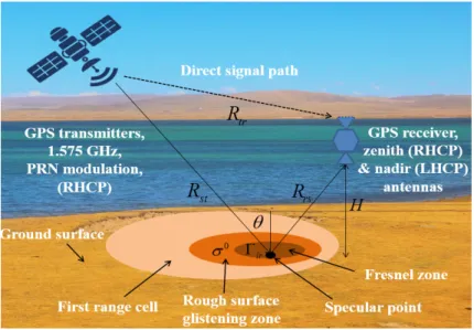
The GPS satellite, ground surface, and receiver constitute a bistatic radar system as described in Figure1. The right-handed circularly polarized antenna receives the direct signal and the left-handed circularly polarized antenna receives the reflected signal. The soil reflectivity is obtained by measuring the power of the reflected GPS signal. In the meanwhile, the surface roughness causes scattering from a glistening zone that contributes to non-coherent power around the specular reflection point. As the roughness increases, the scattering occurs and the incoherent component of the reflected signal increases. For perfect flat surfaces, Fresnel reflection is satisfied and the received power are coherent. As we assumed a smooth surface in this study, the power we received is predominated with LHCP coherent component. Then the soil moisture retrieval method using reflected signal power is based on the inversion of the bistatic radar equation:
Pclr= PtGt 4π(Rst+Rrs)2
Grλ2
4π Γlr (1)
where subscriptlrrepresents the scattering when the satellite incident signal is right-hand polarized and inverts the polarization to LH after surface reflection,Ptis the power of the transmitted signal, Gtis the transmitter antenna gain,Gr is the gain of the receiver antenna, andλis the wavelength (19.042 cm for GPS L1 signal). RrsandRstis the distance between the receiver, the specular point, and the satellite respectively.Γlris the power reflectivity of the reflecting surface.
Remote Sens.2019,11, 1655 5 of 25
Remote Sens. 2019, 11, x FOR PEER REVIEW 5 of 26
Figure 1. Bistatic radar geometry.
The term
Γ
lr in Equation (1) (smooth surface) decreases due to increasing roughness, whichcan be written as [48]:
( ) ( )
2 ( )lr θ Rlr θ χ z
Γ = (2)
where
R
lr is the Fresnel reflection coefficient,χ
( )
z
is the probability density function of the surfaceheight. In the condition of the flat surface χ
( )
z =1, the reflectivity Γlr becomes the amplitudesquared of the Fresnel reflection coefficient
R
lr.Combining (1) and (2), the processed SNR of peak power can be written as:
( ) (
)
2 2 2 2|
|
4
c t t r lr p r p refl peak lr n st rs nP G
P G G G
SNR
R
P
R
R
P
λ
π
=
=
+
(3)where Pn is the noise power and GP is the processing gain due to the de-spread of the GPS C/A code.
The Fresnel reflection coefficient Rlr can be expressed as linear polarization modes [49]:
(
)
1 2
lr rl vv hh
R =R = R −R (4)
where Rh h and Rvv are the Fresnel coefficients for horizontal and vertical polarization [50]:
2 2 cos sin ( ) cos sin r hh r R θ θ ε θ θ ε θ − − = + − (5) 2 2 cos sin ( ) cos sin r r vv r r R θ ε θ ε θ ε θ ε θ − − = + − (6)
where θ is the incident angle, in which
ε
r is the dielectric constant of the surface,0
60
r
j
ε ε ε
=
−
λσ
.ε
0 is the free-space permittivity,σ
is the electric conductivity, and λ is the wavelength. In the case of dry terrain or almost dry, the imaginary part of the permittivity can be neglected [51,52]. With this hypothesis, the real part of the permittivity can be obtained from Equations (3)–(6), when the reflected signals are received [51]. Here the input variables are p e a kr e f le S N R , n
P, Gr, θ respectively as shown in Figure 2.
Figure 1.Bistatic radar geometry.
The termΓlrin Equation (1) (smooth surface) decreases due to increasing roughness, which can be written as [48]: Γlr(θ) = Rlr(θ) 2 χ(z) (2)
whereRlris the Fresnel reflection coefficient,χ(z)is the probability density function of the surface height. In the condition of the flat surfaceχ(z) =1, the reflectivityΓlrbecomes the amplitude squared of the Fresnel reflection coefficientRlr.
Combining (1) and (2), the processed SNR of peak power can be written as:
SNRre f lpeak= P c lrGp Pn = P t rGtGrλ2Gp (4π)2(Rst+Rrs)2Pn |Rlr|2 (3)
wherePnis the noise power andGPis the processing gain due to the de-spread of the GPS C/A code. The Fresnel reflection coefficientRlrcan be expressed as linear polarization modes [49]:
Rlr=Rrl= 1
2(Rvv−Rhh) (4)
whereRhhandRvvare the Fresnel coefficients for horizontal and vertical polarization [50]:
Rhh(θ) = cosθ− pεr−sin2θ cosθ+ pεr−sin2θ (5) Rvv(θ) = εrcosθ −pεr−sin2θ εrcosθ+ p εr−sin2θ (6) whereθis the incident angle, in whichεris the dielectric constant of the surface,εr =ε/ε0−j60λσ. ε0is the free-space permittivity,σis the electric conductivity, andλis the wavelength. In the case of dry terrain or almost dry, the imaginary part of the permittivity can be neglected [51,52]. With this hypothesis, the real part of the permittivity can be obtained from Equations (3)–(6), when the reflected signals are received [51]. Here the input variables areSNRpeakre f le,Pn,Gr,θrespectively as shown in Figure2.
Remote Sens.2019,11, 1655 6 of 25
Remote Sens. 2019, 11, x FOR PEER REVIEW 6 of 26
In Figure 2, the soil reflectivity is obtained by calculating the correlation power of both the reflected signal and the direct signal. In this study, a coherent integration (1 ms) was determined by the length of the GPS PRN (pseudorandom noise) code sequence. Generally, due to the attenuation of signal power caused by surface reflection and the presence of fading noise introduced by surface scattering, 1 ms of integration is not enough to get the correlation peak, consecutive 1 ms coherent correlations must be averaged. This process is known as non-coherent integration. There is not a defined rule governing the choice but it should only be determined by the specific application and by its own situation. In this study, 500 ms of non-coherent integration time is used since it is examined to be long enough to eliminate the effects of speckle noise and short enough to have a good resolution of the surface by multiple experiments. After that, the reflectivity is used to obtain the permittivity through the bistatic radar equations [53]. We must note that the permittivity is strongly related to the soil moisture content. The relationship between soil permittivity and soil moisture is given by the soil permittivity models. Due to its complex structure, simplified empirical or semi-empirical models are used as a function of permittivity in practical applications [54–56].
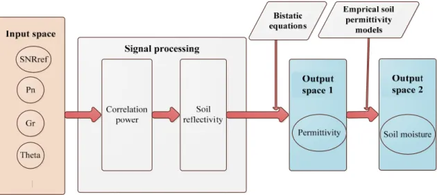
Figure 2. The flowchart of global navigation satellite system-reflectometry (GNSS-R) soil moisture retrieval procedure.
The performance of GNSS-R soil moisture retrieval is an important issue, which is determined by many factors: (1) The geometric and physical characteristics of the reflected surface, such as the statistical distribution of the ground height, the composition of the soil, etc., which impact the received SNR. (2) Parameters of the GNSS-R system, such as the behavior of the transmitting and receiving antennas (Gr, Pn), and the elevation angle (θ ), etc. Except for the above-concerned parameters (input variables), some random factors, the appearance of the surface roughness, vegetation, e.g., leaf orientation, height of the vegetation, etc., may influence the signal collection in the real case. Due to the complex interaction of these parameters, the retrieval of soil moisture content using GNSS-R is commonly based on semi-empirical models. The random factors can be regarded as system noise and suppressed by machine learning methods. Here we considered the retrieval procedure as a nonlinear regression problem with the input variables (SNR, Pn…) and output variables (permittivity, soil moisture) based on the early work [46] as shown in Figure 2.
2.2. XGboost
XGBoost is an improved algorithm based on the gradient-enhanced decision tree, which can effectively construct enhanced trees and run parallel computing. Compared with the traditional GBDT (gradient boosting decision tree) algorithm that only uses the first-order derivative information, the XGBoost performs the second-order Taylor expansion on the loss function and provides higher efficiency of solving the optimal solution [44].
Figure 2. The flowchart of global navigation satellite system-reflectometry (GNSS-R) soil moisture retrieval procedure.
In Figure2, the soil reflectivity is obtained by calculating the correlation power of both the reflected signal and the direct signal. In this study, a coherent integration (1 ms) was determined by the length of the GPS PRN (pseudorandom noise) code sequence. Generally, due to the attenuation of signal power caused by surface reflection and the presence of fading noise introduced by surface scattering, 1 ms of integration is not enough to get the correlation peak, consecutive 1 ms coherent correlations must be averaged. This process is known as non-coherent integration. There is not a defined rule governing the choice but it should only be determined by the specific application and by its own situation. In this study, 500 ms of non-coherent integration time is used since it is examined to be long enough to eliminate the effects of speckle noise and short enough to have a good resolution of the surface by multiple experiments. After that, the reflectivity is used to obtain the permittivity through the bistatic radar equations [53]. We must note that the permittivity is strongly related to the soil moisture content. The relationship between soil permittivity and soil moisture is given by the soil permittivity models. Due to its complex structure, simplified empirical or semi-empirical models are used as a function of permittivity in practical applications [54–56].
The performance of GNSS-R soil moisture retrieval is an important issue, which is determined by many factors: (1) The geometric and physical characteristics of the reflected surface, such as the statistical distribution of the ground height, the composition of the soil, etc., which impact the received SNR. (2) Parameters of the GNSS-R system, such as the behavior of the transmitting and receiving antennas (Gr,Pn), and the elevation angle (θ), etc. Except for the above-concerned parameters (input variables), some random factors, the appearance of the surface roughness, vegetation, e.g., leaf orientation, height of the vegetation, etc., may influence the signal collection in the real case. Due to the complex interaction of these parameters, the retrieval of soil moisture content using GNSS-R is commonly based on semi-empirical models. The random factors can be regarded as system noise and suppressed by machine learning methods. Here we considered the retrieval procedure as a nonlinear regression problem with the input variables (SNR,Pn. . . ) and output variables (permittivity, soil moisture) based on the early work [46] as shown in Figure2.
2.2. XGboost
XGBoost is an improved algorithm based on the gradient-enhanced decision tree, which can effectively construct enhanced trees and run parallel computing. Compared with the traditional GBDT (gradient boosting decision tree) algorithm that only uses the first-order derivative information, the XGBoost performs the second-order Taylor expansion on the loss function and provides higher efficiency of solving the optimal solution [44].
Remote Sens.2019,11, 1655 7 of 25
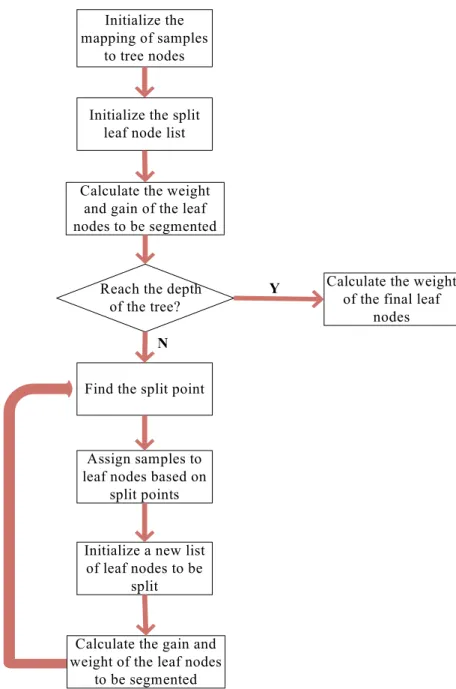
The flowchart of the XGBoost algorithm [42] is summarized in Figure3.
Remote Sens. 2019, 11, x FOR PEER REVIEW 7 of 26
The flowchart of the XGBoost algorithm [42] is summarized in Figure 3.
Initialize the mapping of samples
to tree nodes
Initialize the split leaf node list
Calculate the weight and gain of the leaf nodes to be segmented
Reach the depth of the tree?
Calculate the weight of the final leaf
nodes
Y
Find the split point
N
Assign samples to leaf nodes based on
split points
Initialize a new list of leaf nodes to be
split
Calculate the gain and weight of the leaf nodes
to be segmented
Figure 3. The flowchart of XGBoost algorithm.
Advantages of XGBoost [44]:
(1) Using the second-order Taylor expression to approximate the objective function, making it easier to find the optimal solution;
(2) It can handle sparse and missing data;
(3) Generating a decision tree using the structural score;
(4) The split node uses the candidate set so that the algorithm runs fast;
(5) Define the complexity of the tree and apply it to the objective function to grasp the complexity of the model;
(6) Over-fitting can be prevented by samplings of column features.
The XGBoost also has some disadvantages: The complexity is slightly higher for using XGB to do the feature importance sorting because XGB uses level-wise to generate decision trees. It splits the leaves of the same layer at the same time, thus performing multi-thread optimization, which can avoid overfitting. The traversal selects the optimal segmentation point. When the amount of data is large, the method is time-consuming [57,58].
Figure 3.The flowchart of XGBoost algorithm.
Advantages of XGBoost [44]:
(1) Using the second-order Taylor expression to approximate the objective function, making it easier to find the optimal solution;
(2) It can handle sparse and missing data;
(3) Generating a decision tree using the structural score;
(4) The split node uses the candidate set so that the algorithm runs fast;
(5) Define the complexity of the tree and apply it to the objective function to grasp the complexity of the model;
(6) Over-fitting can be prevented by samplings of column features.
The XGBoost also has some disadvantages: The complexity is slightly higher for using XGB to do the feature importance sorting because XGB uses level-wise to generate decision trees. It splits the
Remote Sens.2019,11, 1655 8 of 25
leaves of the same layer at the same time, thus performing multi-thread optimization, which can avoid overfitting. The traversal selects the optimal segmentation point. When the amount of data is large, the method is time-consuming [57,58].
2.3. XGboost for the Variable Importance Assessment
The feature selection of XGBoost is based on the initial feature set to establish the classification model, to examine the performance of the feature in the model, and to obtain the importance of the feature. According to the degree of variable importance to search and evaluate the feature subset, an optimal subset will be generated. It is a kind of embedded and filtered feature selection method [57]. The core of the algorithm is to optimize the value of the objective function. The gradient enhancement construct is enhanced by the tree to intelligently acquire feature scores, indicating the importance of each feature to the training model. In an enhancement tree, the more times a feature is used to make a critical decision, the higher its score. The algorithm calculates the importance by “gain”, “frequency”, and “coverage”. Gain is the primary reference factor that determines the importance of a branch feature. Frequency is the simplification of gain, as measured by the number of occurrences of a feature in all construction trees. Coverage is the relative value of feature observations. In this study, the feature quantity was determined by the “gain” [47].
When doing the feature selection using the XGBoost algorithm, feature importance calculation is integrated into the classification process. A new tree is created in each iteration of the round, and the branch node of the tree is a feature variable. Feature importance is based on a feature can be selected as the split node of the tree. Each time a feature is added to the tree as a split node, all possible split points are enumerated using the greedy method, from which the best split point is selected [58].
The best split point corresponds to the maximum gain, and the gainGain is calculated [47]. Good features and splitting points can improve the squared difference on a single tree. The more improvements, the better the splitting point, the more important this feature is. When all the trees are established, the calculated node importance is averaged in the forest. The more times a feature is selected as a split point, the higher the importance.
For a treeTwithJbranch nodes, ifJis selected as the split variable on this tree, the sum of the mean squared errors on all branch nodestis calculated, e.g., the importance of feature jon this tree is [42]: ˆ I2j(T) = J−1 X t=1 ˆ I2jP(vt= j) (7)
where ˆI2j is the improvement of squared error of a nodet. Setylandyrwith the predicted mean values of the left and right subtrees respectively, andwlandwrare the weights of the nodes of the left and right subtrees respectively [42].
I2(Rl,Rr) = wlwr wl+wr
(yl+yr)2 (8)
By summing the importance of the featurest on each tree and making an average, the final importance can be obtained for forests withMtrees [42]:
It2= 1 M M X m=1 I2t(Tm) (9)
3. Results and Analysis
In this section, we show the GNSS-R soil moisture retrieval performance analysis from two different points of view. The first one is to utilize the XGBoost algorithm to analyze the importance of the input variables. The input variables in GNSS-R are taken as different input features in XGBoost algorithm. The simulated data set are shown considering the GNSS-R bistatic soil moisture retrieval
Remote Sens.2019,11, 1655 9 of 25
equations in the case of flat surface. Then, the variable importance of the input variables is shown and analyzed by means of three different parameter issues. To investigate the contribution of the different input variables to permittivity and soil conditions (including two typical soil types) respectively. For the second part, it focuses on ground-truth measurements. Two different soil compositions and moisture terrain were chosen to do GNSS-R experiments. Some input variables are analyzed mathematically to validate the results obtained by XGBoost, and the performance of GNSS-R soil moisture retrieval is analyzed in details.
3.1. GNSS-R Soil Moisture Retrieval Data Set
The data set was simulated and trained to analyze the performance of the input variables of GNSS-R by using XGBoost. We considered the soil moisture content and the permittivity had a positive correlation, and some established soil permittivity models [54,55] could be used to retrieve the soil moisture from permittivity, so the permittivity is the output variable that we obtained firstly using the bistatic radar equations for observation, under the assumption of a flat surface [53].
The simulated training set mainly consists of the following input vectors: 1. θ, Elevation data (from 35 degrees to 85 degrees);
2. Gr, Receiver Gain (from 2.5 to 3.5 dB);
3. SNRrh, the signal to noise ratio from the reflected channel (from 2 to 26 dB); 4. Pn, the total noise power of the receiver (from−130 to−150 dB).
The range of the input vector was set with the idea of staying as close as possible to the experimental situation. Those variables (θ,Gr,Pn, andSNRrh) were the observables for the variable importance analysis. Other input vectors, such asRr (distance from the transmitter to a specular point),Pt (transmitted power from GPS satellite),Gt(transmitter antenna gain), andGpr(signal processing gain) were constant numbers that depend on the GNSS-R system and were not shown here.
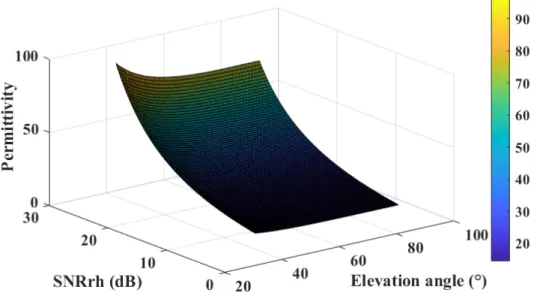
With the GNSS-R retrieval procedure as shown in Figure2, the simulated data were obtained and shown in order to understand the relationship between the SNR, elevation angle, and the permittivity in Figure4. The dataset of Figure4contained 1000 samples. With the increment of the elevation angle and SNR, the permittivity was also increased as shown in Figure4.
Remote Sens. 2019, 11, x FOR PEER REVIEW 9 of 26
respectively. For the second part, it focuses on ground-truth measurements. Two different soil compositions and moisture terrain were chosen to do GNSS-R experiments. Some input variables are analyzed mathematically to validate the results obtained by XGBoost, and the performance of GNSS-R soil moisture retrieval is analyzed in details.
3.1. GNSS-R Soil Moisture Retrieval Data Set
The data set was simulated and trained to analyze the performance of the input variables of GNSS-R by using XGBoost. We considered the soil moisture content and the permittivity had a positive correlation, and some established soil permittivity models [54,55] could be used to retrieve the soil moisture from permittivity, so the permittivity is the output variable that we obtained firstly using the bistatic radar equations for observation, under the assumption of a flat surface [53].
The simulated training set mainly consists of the following input vectors: 1.
θ
, Elevation data (from 35 degrees to 85 degrees);2. Gr, Receiver Gain (from 2.5 to 3.5 dB);
3. SNRrh, the signal to noise ratio from the reflected channel (from 2 to 26 dB); 4. Pn, the total noise power of the receiver (from −130 to −150 dB).
The range of the input vector was set with the idea of staying as close as possible to the experimental situation. Those variables (
θ
, Gr, Pn, and SNRrh ) were the observables for thevariable importance analysis. Other input vectors, such as Rr (distance from the transmitter to a specular point), Pt (transmitted power from GPS satellite), Gt (transmitter antenna gain), and Gpr (signal processing gain) were constant numbers that depend on the GNSS-R system and were not shown here.
With the GNSS-R retrieval procedure as shown in Figure 2, the simulated data were obtained and shown in order to understand the relationship between the SNR, elevation angle, and the permittivity in Figure 4. The dataset of Figure 4 contained 1000 samples. With the increment of the elevation angle and SNR, the permittivity was also increased as shown in Figure 4.
Figure 4. Three-dimensional data set shown for the XGBoost algorithm.
Figure 5a shows the relationship between the SNR and the permittivity when the elevation angle was a constant number (e.g., 84°). Figure 5b considers the relationship between the elevation angle and the permittivity when the SNR was a constant value (20 dB). It is noted that the obtained permittivity was computed from the formulas that comprise the variables SNR and elevation angle [53]. In Figure 5, it was possible to observe a significant result that the permittivity increased with
Figure 4.Three-dimensional data set shown for the XGBoost algorithm.
Figure5a shows the relationship between the SNR and the permittivity when the elevation angle was a constant number (e.g., 84◦). Figure5b considers the relationship between the elevation angle and
Remote Sens.2019,11, 1655 10 of 25
the permittivity when the SNR was a constant value (20 dB). It is noted that the obtained permittivity was computed from the formulas that comprise the variables SNR and elevation angle [53]. In Figure5, it was possible to observe a significant result that the permittivity increased with the increment of the SNR when the elevation angle was a constant value. On the other hand, the permittivity was quite constant for elevation angle ranging between 50◦to 85◦when we fixed the value of the received SNR. The reason is that higher elevation angles lead to higher signal power received. In case of receiving the same SNR (Figure5b), a surface with lower permittivity (lower soil moisture content) requires a signal from a higher elevation angle, compared with a higher permittivity surface.
Remote Sens. 2019, 11, x FOR PEER REVIEW 10 of 26
the increment of the SNR when the elevation angle was a constant value. On the other hand, the permittivity was quite constant for elevation angle ranging between 50° to 85° when we fixed the value of the received SNR. The reason is that higher elevation angles lead to higher signal power received. In case of receiving the same SNR (Figure 5b), a surface with lower permittivity (lower soil moisture content) requires a signal from a higher elevation angle, compared with a higher permittivity surface.
(a) (b)
Figure 5. Two-dimensional data set (a) for the SNR and the permittivity (θ = 84°), two dimensional
data (b) set for the elevation angle and the permittivity (SNR = 20 dB).
3.2. Sensitivity to the Number of Estimators and Samples
XGBoost was performed on the data set, considering the input vectors (SNRrh, Gr Pn, and θ ) and the output vectors (permittivity). Estimators are number of trees to fit and samples n are the numbers of data used. Often the hardest part of solving a machine learning problem can be finding the right estimator for the job. Different estimators are better suited for different types of data and different problems. The figures illustrate the behavior of variable importance estimation for different estimators (500, 4000) and samples, in order to check if the variable importance is still stable when the estimators and the samples n are changed. The samples n were set to 2000 and 5000 (Figure 6).
(a) (b)
Figure 6. Variable importance sensitivity to estimators 500 (a) and 4000 (b) when n = 2000 and
5000.
Figure 5.Two-dimensional data set (a) for the SNR and the permittivity (θ=84◦), two dimensional data (b) set for the elevation angle and the permittivity (SNR=20 dB).
3.2. Sensitivity to the Number of Estimators and Samples
XGBoost was performed on the data set, considering the input vectors (SNRrh,Gr Pn, andθ) and the output vectors (permittivity). Estimators are number of trees to fit and samplesnare the numbers of data used. Often the hardest part of solving a machine learning problem can be finding the right estimator for the job. Different estimators are better suited for different types of data and different problems. The figures illustrate the behavior of variable importance estimation for differentestimators
(500, 4000) and samples, in order to check if the variable importance is still stable when theestimators
and the samplesnare changed. The samplesnwere set to 2000 and 5000 (Figure6).
Remote Sens. 2019, 11, x FOR PEER REVIEW 10 of 26
the increment of the SNR when the elevation angle was a constant value. On the other hand, the permittivity was quite constant for elevation angle ranging between 50° to 85° when we fixed the value of the received SNR. The reason is that higher elevation angles lead to higher signal power received. In case of receiving the same SNR (Figure 5b), a surface with lower permittivity (lower soil moisture content) requires a signal from a higher elevation angle, compared with a higher permittivity surface.
(a) (b)
Figure 5. Two-dimensional data set (a) for the SNR and the permittivity (θ = 84°), two dimensional
data (b) set for the elevation angle and the permittivity (SNR = 20 dB).
3.2. Sensitivity to the Number of Estimators and Samples
XGBoost was performed on the data set, considering the input vectors (SNRrh, Gr Pn, and θ ) and the output vectors (permittivity). Estimators are number of trees to fit and samples n are the
numbers of data used. Often the hardest part of solving a machine learning problem can be finding the right estimator for the job. Different estimators are better suited for different types of data and different problems. The figures illustrate the behavior of variable importance estimation for different estimators (500, 4000) and samples, in order to check if the variable importance is still stable when the estimators and the samples n are changed. The samples n were set to 2000 and 5000 (Figure 6).
(a) (b)
Figure 6. Variable importance sensitivity to estimators 500 (a) and 4000 (b) when n = 2000 and
5000.
Remote Sens.2019,11, 1655 11 of 25
In Figure6, the value of the variableSNRrhwas the highest in these two plots. With the increase of numbers ofestimatorsfrom 500 to 4000, the value ofSNRrhdecreased slightly. Pnandθincreased. We increased the samplesnfrom 2000 to 5000. The variableSNRrhshows the same behavior, andPn,θ increased slightly. Compared Figure6a,b, each column with the same samplesn,Pn, andθincreased, and the value ofSNRrhbecame lower, but it was still the highest among the variables with a value of 0.4 (40%). In addition, the value ofθincreased when the number of theestimatorsand the samples increased but it was still the lowest with a value below 0.1 (10%). In any case, the order of the variable importance was clear and it shows the same importance in those four figures. This phenomenon reports that the value of the variableθ(elevation angle) was much lower thanPn(receiver noise) andGr (receiver gain), which was around 0.1 (10%), indicating that the elevation angle made less contribution to the permittivity retrieval than the other variables. Furthermore, the received SNR was a predominant variable with a contribution over 40% during the permittivity retrieval.
3.3. Sensitivity to the Number of Col-Sample-Tree and Samples
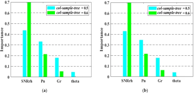
The optimized parametercol−sample−treerepresents the portion of selecting features when building a tree in XGBoost. The choice of thecol−sample−treecan be important for the variable importance estimation. As we showed above, the XGBoost algorithm was performed on the data set considering the input vectors (SNRrh,Gr Pn, andθ) and the output vectors (permittivity). The figures illustrate the behavior of variable importance estimation for differentcol−sample−tree(0.5, 0.6) and samplesn. We tried to check if the variable importance was still stable when the parameters were changed in this case. The samplesnwere set to 2000 and 5000 (Figure7) respectively.
Remote Sens. 2019, 11, x FOR PEER REVIEW 11 of 26
In Figure 6, the value of the variable S N R r h was the highest in these two plots. With the
increase of numbers of estimators from 500 to 4000, the value of S N R r h decreased slightly. Pn and
θ increased. We increased the samples n from 2000 to 5000. The variable S N R r h shows the same behavior, and Pn, θ increased slightly. Compared Figure 6a,b, each column with the same samples
n, Pn, and θ increased, and the value of S N R r h became lower, but it was still the highest among the variables with a value of 0.4 (40%). In addition, the value of θ increased when the number of the estimators and the samples increased but it was still the lowest with a value below 0.1 (10%). In any case, the order of the variable importance was clear and it shows the same importance in those four figures. This phenomenon reports that the value of the variable θ (elevation angle) was much lower than Pn (receiver noise) and Gr (receiver gain), which was around 0.1 (10%), indicating that the elevation angle made less contribution to the permittivity retrieval than the other variables. Furthermore, the received SNR was a predominant variable with a contribution over 40% during the permittivity retrieval.
3.3. Sensitivity to the Number of Col-Sample-Tree and Samples
The optimized parameter col sample tree− − represents the portion of selecting features when building a tree in XGBoost. The choice of the col sample tree− − can be important for the variable importance estimation. As we showed above, the XGBoost algorithm was performed on the data set considering the input vectors (SNRrh, Gr Pn, and θ ) and the output vectors (permittivity). The figures illustrate the behavior of variable importance estimation for different col sample tree− − (0.5, 0.6) and samples n. We tried to check if the variable importance was still stable when the parameters were changed in this case. The samples n were set to 2000 and 5000 (Figure 7) respectively.
(a) (b)
Figure 7. Variable importance sensitivity to col sample tree− − 0.5 (a) and 0.6 (b) for n = 2000 and
5000.
The optimization of parameters can help with differentiating the significant variable and increase the stability of the variable importance estimation. In this case, the value of S N R r h was the highest that was also observed in Figure 7a. When n = 2000, col sample tree− − increased from 0.5 to 0.6, S N R r h increased to a value of 0.6. The value of Gr decreased to 0.1 (10%). The value of θ also decreased to nearly zero. When the samples n = 5000, the variables S N R r h showed the same behavior with the case of n = 2000, and the values of Gr and θ (nearly zero) also decreased. If we increased the samples n from 2000 to 5000, Pn and θ increased little, and the value of S N R r h
Figure 7.Variable importance sensitivity tocol−sample−tree0.5 (a) and 0.6 (b) forn=2000 and 5000.
The optimization of parameters can help with differentiating the significant variable and increase the stability of the variable importance estimation. In this case, the value ofSNRrhwas the highest that was also observed in Figure7a. Whenn=2000,col−sample−treeincreased from 0.5 to 0.6,SNRrh increased to a value of 0.6. The value ofGrdecreased to 0.1 (10%). The value ofθalso decreased to nearly zero. When the samplesn=5000, the variablesSNRrhshowed the same behavior with the case ofn=2000, and the values ofGrandθ(nearly zero) also decreased. If we increased the samplesn from 2000 to 5000,Pnandθincreased little, and the value ofSNRrhdecreased little, but the variable
SNRrhstill showed the highest value among the variables in those plots. Furthermore, the value ofθ is still the lowest value as mentioned before. In any case, the order of the variable importance was clear and quite stable in those four plots. This phenomenon also reported that the received SNR was predominate and the most sensitive parameter to the GNSS-R permittivity retrieval with the maximum contribution of 0.6 (60%). In addition, the value of the variableθ(elevation angle) was much lower
Remote Sens.2019,11, 1655 12 of 25
thanPn(receiver noise) andGr(receiver gain), which could be nearly zero indicating that the variable θwas not very sensitive to the output (permittivity) in this case. It also confirmed that it was a less sensitive input parameter in permittivity retrieval of GNSS-R.
3.4. Sensitivity to Different Types of Soil Compositions
The previous cases illustrate the importance and the sensitivity of the input variables for the permittivity retrieval in GNSS-R. The permittivity has a positive relationship with soil moisture content [54]. The relationship between soil permittivity and soil moisture is given by the soil permittivity models [54–56], so several static measurements were performed by the Remote Sensing Group at Politecnico di Torino in 2016. Among them, two typical types of soils that were chosen intentionally here to investigate the variable importance sensitivity for GNSS-R soil moisture content.
In Tables1and2, the composition (volume percentage and type of sand, clay) of the soil was reported in detail. According to the United States Department of Agriculture (USDA) Classification System, the two types of soil belong to the loamy sand and silty clay loam textural classes, respectively [59]. These different soil compositions that were used in the soil models for the permittivity to retrieve the soil moisture content here, and also for the subsequent ground-truth measurement.
Table 1.Composition of the loamy sand soil (Grugliasco experiment) [53].
Coarse Sand (%) Fine Sand (%) Very Fine Sand (%) Coarse Silt
(%) Fine Silt (%) Clay (%)
Organic Matter (%)
15.5 50.1 16.1 5.3 8.2 4.8 1.4
Table 2.Composition of the silty clay loam soil (Agliano experiment) [53].
Coarse Sand
(%) Fine Sand (%) Coarse Silt (%) Fine Silt (%) Clay (%)
Organic Matter (%)
1.1 10.5 6.4 44.5 36.8 0.7
The parameters of the sensitivity to the permittivity retrieval were studied in the previous case and showed that the order of the variable importance was clear and quite stable. In this case, we illustrated the sensitivity analysis for the input variables to soil moisture retrieval. The more samplesn
we had, the results were more stable and precise, so the optimization parameters wereestimators=2000,
n=5000, regarding the parametercol−sample−tree=0.5 and 0.6 (Figure8) respectively. In Figure8, the loamy sand (a) and silty clay loam soil (b) case had similar behavior. The processedSNRwas the most sensitive parameter and theθwas the opposite. These variables in the two plots illustrated the same order as before. The highest contribution was observed whencol−sample−tree=0.6, with the maximum of the importance of 0.7 (70%). The same as before, the value of the variableθ(elevation angle) was much lower than thePn(receiver noise) andGr(receiver gain), which denotes the minimum value of nearly zero indicating that the variableθwas almost not sensitive to the output (soil moisture content) in this case. It also confirms that it is a less important input parameter in soil moisture retrieval of GNSS-R.
Remote Sens.Remote Sens. 20192019, ,1111, 1655, x FOR PEER REVIEW 13 of 26 13 of 25
(a) (b)
Figure 8. Variable importance sensitivity to different types of soils, Grugliasco (a) and Agliano (b),
when estimators = 2000, n = 5000, col sample tree− − = 0.5 and 0.6. 3.5. Ground-Truth Experiment Data for Validation
Several ground-truth experiments were done in various test sites. Two sets of data particularly with two different typical soil compositions and soil moisture content (dry terrain and a wet terrain) were considered. Two ground-based campaigns with a controlled environment are shown in Figure 9. The first site is located in Grugliasco, Torino (45°03’58.5”N, 7°35’33.8”E), in the Dipartimento Inter-ateneo di Scienze Progetto e Politiche del Territorio (DIST) of Polito. In this place, a wide field of known characteristics (mainly 50% of sand) was available. The second site was located in Agliano (44°47’29.1”N, 8°15’19.8”E), where it is an area of smooth hills mainly devoted to wine production. In this second case, the composition of the soil is 50% silt and 37% clay. The details of the soil compositions for the two sites are reported in Tables 1 and 2.
Figure 9. Two ground-based setups in Grugliasco (left panel) and Agliano (right panel).
During the experiment, GNSS-R equipment and time-domain reflectometry (TDR) setup were used to make measurements before and after rain in bare fields. They were intentionally chosen due to their different terrain composition. The measurements in the dry condition were done after a long drought, and the wet condition was determined after several rainfalls. The timeline of the rainfall and the measurements are shown in Figure 10. The TDR measurement can provide a high spatial resolution between 1.0 and 2.0 cm for SMC between 10% and 40% [60] and reliable permittivity profiles that would be used in the GNSS-R performance analysis [61,62].
Figure 8.Variable importance sensitivity to different types of soils, Grugliasco (a) and Agliano (b), whenestimators=2000,n=5000,col−sample−tree=0.5 and 0.6.
3.5. Ground-Truth Experiment Data for Validation
Several ground-truth experiments were done in various test sites. Two sets of data particularly with two different typical soil compositions and soil moisture content (dry terrain and a wet terrain) were considered. Two ground-based campaigns with a controlled environment are shown in Figure9. The first site is located in Grugliasco, Torino (45◦03058.5”N, 7◦35033.8”E), in the Dipartimento Inter-ateneo di Scienze Progetto e Politiche del Territorio (DIST) of Polito. In this place, a wide field of known characteristics (mainly 50% of sand) was available. The second site was located in Agliano (44◦47029.1”N, 8◦15019.8”E), where it is an area of smooth hills mainly devoted to wine production. In this second case, the composition of the soil is 50% silt and 37% clay. The details of the soil compositions for the two sites are reported in Tables1and2.
Remote Sens. 2019, 11, x FOR PEER REVIEW 13 of 26
(a) (b)
Figure 8. Variable importance sensitivity to different types of soils, Grugliasco (a) and Agliano (b), when estimators = 2000, n = 5000, col sample tree− − = 0.5 and 0.6.
3.5. Ground-Truth Experiment Data for Validation
Several ground-truth experiments were done in various test sites. Two sets of data particularly with two different typical soil compositions and soil moisture content (dry terrain and a wet terrain) were considered. Two ground-based campaigns with a controlled environment are shown in Figure 9. The first site is located in Grugliasco, Torino (45°03’58.5”N, 7°35’33.8”E), in the Dipartimento Inter-ateneo di Scienze Progetto e Politiche del Territorio (DIST) of Polito. In this place, a wide field of known characteristics (mainly 50% of sand) was available. The second site was located in Agliano (44°47’29.1”N, 8°15’19.8”E), where it is an area of smooth hills mainly devoted to wine production. In this second case, the composition of the soil is 50% silt and 37% clay. The details of the soil compositions for the two sites are reported in Tables 1 and 2.
Figure 9. Two ground-based setups in Grugliasco (left panel) and Agliano (right panel).
During the experiment, GNSS-R equipment and time-domain reflectometry (TDR) setup were used to make measurements before and after rain in bare fields. They were intentionally chosen due to their different terrain composition. The measurements in the dry condition were done after a long drought, and the wet condition was determined after several rainfalls. The timeline of the rainfall and the measurements are shown in Figure 10. The TDR measurement can provide a high spatial resolution between 1.0 and 2.0 cm for SMC between 10% and 40% [60] and reliable permittivity profiles that would be used in the GNSS-R performance analysis [61,62].
Figure 9.Two ground-based setups in Grugliasco (leftpanel) and Agliano (rightpanel).
During the experiment, GNSS-R equipment and time-domain reflectometry (TDR) setup were used to make measurements before and after rain in bare fields. They were intentionally chosen due to their different terrain composition. The measurements in the dry condition were done after a long drought, and the wet condition was determined after several rainfalls. The timeline of the rainfall and the measurements are shown in Figure10. The TDR measurement can provide a high spatial resolution between 1.0 and 2.0 cm for SMC between 10% and 40% [60] and reliable permittivity profiles that would be used in the GNSS-R performance analysis [61,62].
Remote Sens.2019,11, 1655 14 of 25
Remote Sens. 2019, 11, x FOR PEER REVIEW 14 of 26
Precipitations in Grugliasco and Agliano
Figure 10. Precipitations in Grugliasco and Agliano during January to March 2016.
The GNSS-R system consists of two commercial frontends connected to two antennas and PCs for data acquisition. It was performed in bistatic GNSS-R configuration, which has one right-hand (RH) antenna pointing to the sky for receiving the direct signal and another left-hand (LH) antenna pointed downwards to receive the reflected signals in Figure 9. The antennas used in the experimental were two commercial antennas produced by ANTCOM Corp. that were able to receive the GNSS signals in L1 and L2 bands. Two commercial front-end SiGe GN3S v2 USB RF developed by the Colorado Center for Astrodynamics Research were used [63]. The front-end connected to the two antennas and a cable was used to transfer the sampled data to a PC. The antennas were mounted on a plastic tripod. The board was installed on the end of the bar that was kept horizontal at a height of 1.45 in both places (Grugliasco and Agliano). The acquisition of GPS data was performed by using N-Grab GNSS data grabber that was developed by the NavSAS group of Polito di Torino [64]. Then the raw data were post-processed for obtaining the SNR of each satellite. The reflected signals mainly contained the LH signal, and this measurement was done in the condition regardless of the surface roughness and incoherent components.
The values of the permittivity are obtained from local measurements based on time-domain reflectometry (TDR) technique [62]. A rod sensor (length 15 cm) Tektronix Metallic Cable Tester 1502 manufactured by Tektronix Inc., Beaverton, OR, USA, was used in the measurements (Figure 11). Then the value of permittivity was obtained from the travel time of the TDR probe. In this measurement, the position of the TDR probe was tilted to 30° with respect to the surface, thus, only around 7 cm of the surface were taken into account in the TDR measurements. This was done in order to satisfy the TDR results with those obtained with GNSS-R that sense only the first few centimeters of the surface (2–5 cm).
Figure 11. Tektronix Metallic Cable Tester 1502 for time-domain reflectometry (TDR) measurements. In the GNSS-R measurements, the major axis of the first Fresnel zone (the region surrounding the specular point from, which power is reflected with a phase change across the surface constrained to π radians, see Figure 1), for satellites in our geometrical condition (high elevation angle and a height of tripod of 1.5 m) was around 1 m. The TDR portable system was moved around to cover this
Figure 10.Precipitations in Grugliasco and Agliano during January to March 2016.
The GNSS-R system consists of two commercial frontends connected to two antennas and PCs for data acquisition. It was performed in bistatic GNSS-R configuration, which has one right-hand (RH) antenna pointing to the sky for receiving the direct signal and another left-hand (LH) antenna pointed downwards to receive the reflected signals in Figure9. The antennas used in the experimental were two commercial antennas produced by ANTCOM Corp. that were able to receive the GNSS signals in L1 and L2 bands. Two commercial front-end SiGe GN3S v2 USB RF developed by the Colorado Center for Astrodynamics Research were used [63]. The front-end connected to the two antennas and a cable was used to transfer the sampled data to a PC. The antennas were mounted on a plastic tripod. The board was installed on the end of the bar that was kept horizontal at a height of 1.45 in both places (Grugliasco and Agliano). The acquisition of GPS data was performed by using N-Grab GNSS data grabber that was developed by the NavSAS group of Polito di Torino [64]. Then the raw data were post-processed for obtaining the SNR of each satellite. The reflected signals mainly contained the LH signal, and this measurement was done in the condition regardless of the surface roughness and incoherent components.
The values of the permittivity are obtained from local measurements based on time-domain reflectometry (TDR) technique [62]. A rod sensor (length 15 cm) Tektronix Metallic Cable Tester 1502 manufactured by Tektronix Inc., Beaverton, OR, USA, was used in the measurements (Figure11). Then the value of permittivity was obtained from the travel time of the TDR probe. In this measurement, the position of the TDR probe was tilted to 30◦with respect to the surface, thus, only around 7 cm of the surface were taken into account in the TDR measurements. This was done in order to satisfy the TDR results with those obtained with GNSS-R that sense only the first few centimeters of the surface (2–5 cm).
Remote Sens. 2019, 11, x FOR PEER REVIEW 14 of 26
Precipitations in Grugliasco and Agliano
Figure 10. Precipitations in Grugliasco and Agliano during January to March 2016.
The GNSS-R system consists of two commercial frontends connected to two antennas and PCs for data acquisition. It was performed in bistatic GNSS-R configuration, which has one right-hand (RH) antenna pointing to the sky for receiving the direct signal and another left-hand (LH) antenna pointed downwards to receive the reflected signals in Figure 9. The antennas used in the experimental were two commercial antennas produced by ANTCOM Corp. that were able to receive the GNSS signals in L1 and L2 bands. Two commercial front-end SiGe GN3S v2 USB RF developed by the Colorado Center for Astrodynamics Research were used [63]. The front-end connected to the two antennas and a cable was used to transfer the sampled data to a PC. The antennas were mounted on a plastic tripod. The board was installed on the end of the bar that was kept horizontal at a height of 1.45 in both places (Grugliasco and Agliano). The acquisition of GPS data was performed by using N-Grab GNSS data grabber that was developed by the NavSAS group of Polito di Torino [64]. Then the raw data were post-processed for obtaining the SNR of each satellite. The reflected signals mainly contained the LH signal, and this measurement was done in the condition regardless of the surface roughness and incoherent components.
The values of the permittivity are obtained from local measurements based on time-domain reflectometry (TDR) technique [62]. A rod sensor (length 15 cm) Tektronix Metallic Cable Tester 1502 manufactured by Tektronix Inc., Beaverton, OR, USA, was used in the measurements (Figure 11). Then the value of permittivity was obtained from the travel time of the TDR probe. In this measurement, the position of the TDR probe was tilted to 30° with respect to the surface, thus, only around 7 cm of the surface were taken into account in the TDR measurements. This was done in order to satisfy the TDR results with those obtained with GNSS-R that sense only the first few centimeters of the surface (2–5 cm).
Figure 11. Tektronix Metallic Cable Tester 1502 for time-domain reflectometry (TDR) measurements.
In the GNSS-R measurements, the major axis of the first Fresnel zone (the region surrounding the specular point from, which power is reflected with a phase change across the surface constrained to π radians, see Figure 1), for satellites in our geometrical condition (high elevation angle and a height of tripod of 1.5 m) was around 1 m. The TDR portable system was moved around to cover this area. Five measurements are performed with a cross scheme as shown in Figure 11 and the results are the averages of the five (black circles).
Figure 11.Tektronix Metallic Cable Tester 1502 for time-domain reflectometry (TDR) measurements.
In the GNSS-R measurements, the major axis of the first Fresnel zone (the region surrounding the specular point from, which power is reflected with a phase change across the surface constrained toπ radians, see Figure1), for satellites in our geometrical condition (high elevation angle and a height of tripod of 1.5 m) was around 1 m. The TDR portable system was moved around to cover this area. Five measurements are performed with a cross scheme as shown in Figure11and the results are the averages of the five (black circles).
Remote Sens.2019,11, 1655 15 of 25
Table 3.Summary of the experimental campaign.
Date Soil Condition Location Soil Type
27 January 2016 Dry condition Grugliasco Loamy sand 5 February 2016 Dry condition Agliano Silty clay loam soil
3 March 2016 Wet condition Grugliasco Loamy sand 7 March 2016 Wet condition Agliano Silty clay loam soil
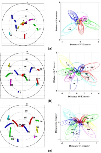
The traces of satellites in the sky during the experiment are plotted using different colors as shown in the skyplot of Figure12. It shows the positions of satellites in terms of elevation and azimuth. The elevation was scaled by the concentric rings nested within one another. The outside ring was 0◦and the middle of the plot was a 90◦elevation. The azimuth is the direction angle with respect to the North (0◦) measured clockwise. The sky plot for experiments in Grugliasco and Agliano was determined before each measurement to choose a proper system position and obtain the input variable (ϑ). Especially, for static measurements, when the receiver is only a few meters high above the ground, the knowledge of the positions of the satellites and the first Fresnel zone coverage is sometimes crucial for analyzing the obtained data and provide the range of the data for comparing the results with other kinds of measurements. Here we also added the information of the position of the receiver and the direction that the bar was pointing to, which greatly helped with the GNSS-R retrieval analysis.
Remote Sens. 2019, 11, x FOR PEER REVIEW 16 of 26
Table 3. Summary of the experimental campaign.
Date Soil condition Location Soil Type
27 January 2016 Dry condition Grugliasco Loamy sand 5 February 2016 Dry condition Agliano Silty clay loam soil
3 March 2016 Wet condition Grugliasco Loamy sand 7 March 2016 Wet condition Agliano Silty clay loam soil
The traces of satellites in the sky during the experiment are plotted using different colors as shown in the skyplot of Figure 12. It shows the positions of satellites in terms of elevation and azimuth. The elevation was scaled by the concentric rings nested within one another. The outside ring was 0° and the middle of the plot was a 90° elevation. The azimuth is the direction angle with respect to the North (0°) measured clockwise. The sky plot for experiments in Grugliasco and Agliano was determined before each measurement to choose a proper system position and obtain the input variable (ϑ). Especially, for static measurements, when the receiver is only a few meters high above the ground, the knowledge of the positions of the satellites and the first Fresnel zone coverage is sometimes crucial for analyzing the obtained data and provide the range of the data for comparing the results with other kinds of measurements. Here we also added the information of the position of the receiver and the direction that the bar was pointing to, which greatly helped with the GNSS-R retrieval analysis.
(a)
(b)
(c) Figure 12.Cont.


![Table 1. Composition of the loamy sand soil (Grugliasco experiment) [53].](https://thumb-us.123doks.com/thumbv2/123dok_us/10012000.2493594/13.892.136.762.508.567/table-composition-loamy-sand-soil-grugliasco-experiment.webp)