Elementary Differential Equations with Boundary Value Problems

(1)

ELEMENTARY

DIFFERENTIAL EQUATIONS WITH

BOUNDARY VALUE PROBLEMS

William F. Trench

Andrew G. Cowles Distinguished Professor Emeritus

Department of Mathematics

Trinity University

San Antonio, Texas, USA

wtrench@trinity.edu

This book has been judged to meet the evaluation criteria set by the

Edi-torial Board of the American Institute of Mathematics in connection with

the Institute’s

Open Textbook Initiative. It may be copied, modified,

re-distributed, translated, and built upon subject to the Creative Commons

Attribution-NonCommercial-ShareAlike 3.0 Unported License.

(2)

Free Edition 1.01 (December 2013)

(3)

(4)

Preface

Elementary Differential Equations with Boundary Value Problemsis written for students in science,

en-gineering, and mathematics who have completed calculus through partial differentiation. If your syllabus includes Chapter 10 (Linear Systems of Differential Equations), your students should have some prepa-ration in linear algebra.

In writing this book I have been guided by the these principles:

• An elementary text should be written so the student can read it with comprehension without too much pain. I have tried to put myself in the student’s place, and have chosen to err on the side of too much detail rather than not enough.

• An elementary text can’t be better than its exercises. This text includes 2041 numbered exercises, many with several parts. They range in difficulty from routine to very challenging.

• An elementary text should be written in an informal but mathematically accurate way, illustrated by appropriate graphics. I have tried to formulate mathematical concepts succinctly in language that students can understand. I have minimized the number of explicitly stated theorems and def-initions, preferring to deal with concepts in a more conversational way, copiously illustrated by 299 completely worked out examples. Where appropriate, concepts and results are depicted in 188 figures.

Although I believe that the computer is an immensely valuable tool for learning, doing, and writing mathematics, the selection and treatment of topics in this text reflects my pedagogical orientation along traditional lines. However, I have incorporated what I believe to be the best use of modern technology, so you can select the level of technology that you want to include in your course. The text includes 414 exercises – identified by the symbols C and C/G – that call for graphics or computation and graphics. There are also 79 laboratory exercises – identified by L – that require extensive use of technology. In addition, several sections include informal advice on the use of technology. If you prefer not to emphasize technology, simply ignore these exercises and the advice.

There are two schools of thought on whether techniques and applications should be treated together or separately. I have chosen to separate them; thus, Chapter 2 deals with techniques for solving first order equations, and Chapter 4 deals with applications. Similarly, Chapter 5 deals with techniques for solving second order equations, and Chapter 6 deals with applications. However, the exercise sets of the sections dealing with techniques include some applied problems.

Traditionally oriented elementary differential equations texts are occasionally criticized as being col-lections of unrelated methods for solving miscellaneous problems. To some extent this is true; after all, no single method applies to all situations. Nevertheless, I believe that one idea can go a long way toward unifying some of the techniques for solving diverse problems: variation of parameters. I use variation of parameters at the earliest opportunity in Section 2.1, to solve the nonhomogeneous linear equation, given a nontrivial solution of the complementary equation. You may find this annoying, since most of us learned that one should use integrating factors for this task, while perhaps mentioning the variation of parameters option in an exercise. However, there’s little difference between the two approaches, since an integrating factor is nothing more than the reciprocal of a nontrivial solution of the complementary equation. The advantage of using variation of parameters here is that it introduces the concept in its simplest form and

(8)

viii Preface

focuses the student’s attention on the idea of seeking a solutionyof a differential equation by writing it asy=uy1, wherey1is a known solution of related equation anduis a function to be determined. I use this idea in nonstandard ways, as follows:

• In Section 2.4 to solve nonlinear first order equations, such as Bernoulli equations and nonlinear homogeneous equations.

• In Chapter 3 for numerical solution of semilinear first order equations.

• In Section 5.2 to avoid the necessity of introducing complex exponentials in solving a second or-der constant coefficient homogeneous equation with characteristic polynomials that have complex zeros.

• In Sections 5.4, 5.5, and 9.3 for the method of undetermined coefficients. (If the method of an-nihilators is your preferred approach to this problem, compare the labor involved in solving, for example,y00₊_y0₊_y₌_x4_ex_{by the method of annihilators and the method used in Section 5.4.)}

Introducing variation of parameters as early as possible (Section 2.1) prepares the student for the con-cept when it appears again in more complex forms in Section 5.6, where reduction of order is used not merely to find a second solution of the complementary equation, but also to find the general solution of the nonhomogeneous equation, and in Sections 5.7, 9.4, and 10.7, that treat the usual variation of parameters problem for second and higher order linear equations and for linear systems.

Chapter 11 develops the theory of Fourier series. Section 11.1 discusses the five main eigenvalue prob-lems that arise in connection with the method of separation of variables for the heat and wave equations and for Laplace’s equation over a rectangular domain:

Problem 1: y00₊_λy_{= 0}_, _y_{(0) = 0}_, _y₍_L_{) = 0}

Problem 2: y00₊_λy_{= 0}_, _y0_{(0) = 0}_, _y0₍_L_{) = 0}

Problem 3: y00₊_λy_{= 0}_, _y_{(0) = 0}_, _y0₍_L_{) = 0}

Problem 4: y00₊_λy_{= 0}_, _y0_{(0) = 0}_, _y₍_L_{) = 0}

Problem 5: y00₊_λy_{= 0}_, _y₍₋_L_{) =}_y₍_L₎_, _y0₍₋_L_{) =}_y0₍_L₎

These problems are handled in a unified way for example, a single theorem shows that the eigenvalues of all five problems are nonnegative.

Section 11.2 presents the Fourier series expansion of functions defined on on[−L, L], interpreting it as an expansion in terms of the eigenfunctions of Problem 5.

Section 11.3 presents the Fourier sine and cosine expansions of functions defined on[0, L], interpreting them as expansions in terms of the eigenfunctions of Problems 1 and 2, respectively. In addition, Sec-tion 11.2 includes what I call the mixed Fourier sine and cosine expansions, in terms of the eigenfuncSec-tions of Problems 4 and 5, respectively. In all cases, the convergence properties of these series are deduced from the convergence properties of the Fourier series discussed in Section 11.1.

Chapter 12 consists of four sections devoted to the heat equation, the wave equation, and Laplace’s equation in rectangular and polar coordinates. For all three, I consider homogeneous boundary conditions of the four types occurring in Problems 1-4. I present the method of separation of variables as a way of choosing the appropriate form for the series expansion of the solution of the given problem, stating— without belaboring the point—that the expansion may fall short of being an actual solution, and giving an indication of conditions under which the formal solution is an actual solution. In particular, I found it necessary to devote some detail to this question in connection with the wave equation in Section 12.2.

(9)

the homogeneous boundary conditions. Similarly, in most of the examples and exercises Section 12.3 (Laplace’s Equation), the functions defining the boundary conditions on a given side of the rectangular domain satisfy homogeneous boundary conditions at the endpoints of the same type (Dirichlet or Neu-mann) as the boundary conditions imposed on adjacent sides of the region. Therefore the formal solutions obtained in many of the examples and exercises are actual solutions.

Section 13.1 deals with two-point value problems for a second order ordinary differential equation. Conditions for existence and uniqueness of solutions are given, and the construction of Green’s functions is included.

Section 13.2 presents the elementary aspects of Sturm-Liouville theory. You may also find the following to be of interest:

• Section 2.6 deals with integrating factors of the formµ = p(x)q(y), in addition to those of the formµ=p(x)andµ=q(y)discussed in most texts.

• Section 4.4 makes phase plane analysis of nonlinear second order autonomous equations accessi-ble to students who have not taken linear algebra, since eigenvalues and eigenvectors do not enter into the treatment. Phase plane analysis of constant coefficient linear systems is included in Sec-tions 10.4-6.

• Section 4.5 presents an extensive discussion of applications of differential equations to curves.

• Section 6.4 studies motion under a central force, which may be useful to students interested in the mathematics of satellite orbits.

• Sections 7.5-7 present the method of Frobenius in more detail than in most texts. The approach is to systematize the computations in a way that avoids the necessity of substituting the unknown Frobenius series into each equation. This leads to efficiency in the computation of the coefficients of the Frobenius solution. It also clarifies the case where the roots of the indicial equation differ by an integer (Section 7.7).

• The free Student Solutions Manual contains solutions of most of the even-numbered exercises.

• The free Instructor’s Solutions Manual is available by email towtrench@trinity.edu, subject to verification of the requestor’s faculty status.

The following observations may be helpful as you choose your syllabus:

• Section 2.3 is the only specific prerequisite for Chapter 3. To accomodate institutions that offer a separate course in numerical analysis, Chapter 3 is not a prerequisite for any other section in the text.

• The sections in Chapter 4 are independent of each other, and are not prerequisites for any of the later chapters. This is also true of the sections in Chapter 6, except that Section 6.1 is a prerequisite for Section 6.2.

• Chapters 7, 8, and 9 can be covered in any order after the topics selected from Chapter 5. For example, you can proceed directly from Chapter 5 to Chapter 9.

• The second order Euler equation is discussed in Section 7.4, where it sets the stage for the method of Frobenius. As noted at the beginning of Section 7.4, if you want to include Euler equations in your syllabus while omitting the method of Frobenius, you can skip the introductory paragraphs in Section 7.4 and begin with Definition 7.4.2. You can then cover Section 7.4 immediately after Section 5.2.

• Chapters 11, 12, and 13 can be covered at any time after the completion of Chapter 5.

(10)

CHAPTER 1 Introduction

IN THIS CHAPTER we begin our study of differential equations.

SECTION 1.1 presents examples of applications that lead to differential equations.

SECTION 1.2 introduces basic concepts and definitions concerning differential equations.

SECTION 1.3 presents a geometric method for dealing with differential equations that has been known for a very long time, but has become particularly useful and important with the proliferation of readily available differential equations software.

(11)

1.1 APPLICATIONS LEADING TO DIFFERENTIAL EQUATIONS

In order to apply mathematical methods to a physical or “real life” problem, we must formulate the prob-lem in mathematical terms; that is, we must construct a mathematical model for the problem. Many physical problems concern relationships between changing quantities. Since rates of change are repre-sented mathematically by derivatives, mathematical models often involve equations relating an unknown function and one or more of its derivatives. Such equations aredifferential equations. They are the subject of this book.

Much of calculus is devoted to learning mathematical techniques that are applied in later courses in mathematics and the sciences; you wouldn’t have time to learn much calculus if you insisted on seeing a specific application of every topic covered in the course. Similarly, much of this book is devoted to methods that can be applied in later courses. Only a relatively small part of the book is devoted to the derivation of specific differential equations from mathematical models, or relating the differential equations that we study to specific applications. In this section we mention a few such applications.

The mathematical model for an applied problem is almost always simpler than the actual situation being studied, since simplifying assumptions are usually required to obtain a mathematical problem that can be solved. For example, in modeling the motion of a falling object, we might neglect air resistance and the gravitational pull of celestial bodies other than Earth, or in modeling population growth we might assume that the population grows continuously rather than in discrete steps.

A good mathematical model has two important properties:

• It’s sufficiently simple so that the mathematical problem can be solved.

• It represents the actual situation sufficiently well so that the solution to the mathematical problem predicts the outcome of the real problem to within a useful degree of accuracy. If results predicted by the model don’t agree with physical observations, the underlying assumptions of the model must be revised until satisfactory agreement is obtained.

We’ll now give examples of mathematical models involving differential equations. We’ll return to these problems at the appropriate times, as we learn how to solve the various types of differential equations that occur in the models.

All the examples in this section deal with functions of time, which we denote byt. Ifyis a function of t,y0_{denotes the derivative of}_y_{with respect to}_{t; thus,}

y0₌ dy

dt.

Population Growth and Decay

Although the number of members of a population (people in a given country, bacteria in a laboratory cul-ture, wildflowers in a forest, etc.) at any given timetis necessarily an integer, models that use differential equations to describe the growth and decay of populations usually rest on the simplifying assumption that the number of members of the population can be regarded as a differentiable functionP=P(t). In most models it is assumed that the differential equation takes the form

P0₌_a₍_P₎_P,

(1.1.1)

whereais a continuous function ofP that represents the rate of change of population per unit time per individual. In theMalthusian model, it is assumed thata(P)is a constant, so (1.1.1) becomes

(12)

Section 1.1 Applications Leading to Differential Equations 3

(When you see a name in blue italics, just click on it for information about the person.) This model assumes that the numbers of births and deaths per unit time are both proportional to the population. The constants of proportionality are thebirth rate (births per unit time per individual) and the death rate

(deaths per unit time per individual);ais the birth rate minus the death rate. You learned in calculus that ifcis any constant then

P =ceat (1.1.3)

satisfies (1.1.2), so (1.1.2) has infinitely many solutions. To select the solution of the specific problem that we’re considering, we must know the populationP0at an initial time, sayt = 0. Settingt= 0in (1.1.3) yieldsc=P(0) =P0, so the applicable solution is

P(t) =P0eat.

This implies that

lim

t→∞P(t) =

∞ ifa >0,

0 ifa <0;

that is, the population approaches infinity if the birth rate exceeds the death rate, or zero if the death rate exceeds the birth rate.

To see the limitations of the Malthusian model, suppose we’re modeling the population of a country, starting from a timet = 0when the birth rate exceeds the death rate (so a > 0), and the country’s resources in terms of space, food supply, and other necessities of life can support the existing popula-tion. Then the predictionP = P0eat _{may be reasonably accurate as long as it remains within limits} that the country’s resources can support. However, the model must inevitably lose validity when the pre-diction exceeds these limits. (If nothing else, eventually there won’t be enough space for the predicted population!)

This flaw in the Malthusian model suggests the need for a model that accounts for limitations of space and resources that tend to oppose the rate of population growth as the population increases. Perhaps the most famous model of this kind is theVerhulst model, where (1.1.2) is replaced by

P0 ₌_aP₍₁

−αP), (1.1.4)

whereαis a positive constant. As long asPis small compared to1/α, the ratioP0_/P _{is approximately}

equal toa. Therefore the growth is approximately exponential; however, asP increases, the ratioP0_/P

decreases as opposing factors become significant.

Equation (1.1.4) is thelogistic equation. You will learn how to solve it in Section 1.2. (See Exer-cise 2.2.28.) The solution is

P = P0

αP0+ (1−αP0)e−at,

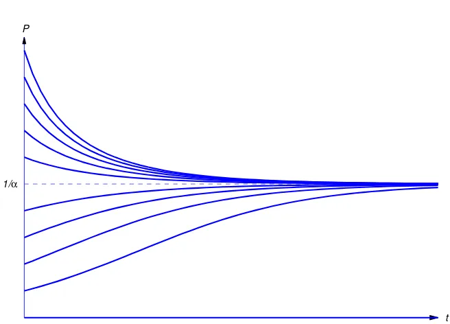
whereP0=P(0)>0. Thereforelimt→∞P(t) = 1/α, independent ofP0.

Figure1.1.1shows typical graphs ofPversustfor various values ofP0. Newton’s Law of Cooling

According toNewton’s law of cooling, the temperature of a body changes at a rate proportional to the difference between the temperature of the body and the temperature of the surrounding medium. Thus, if Tmis the temperature of the medium andT =T(t)is the temperature of the body at timet, then

T0₌

−k(T −Tm), (1.1.5)

wherekis a positive constant and the minus sign indicates; that the temperature of the body increases with time if it’s less than the temperature of the medium, or decreases if it’s greater. We’ll see in Section 4.2 that ifTmis constant then the solution of (1.1.5) is

(13)

P

[image:13.612.141.469.94.330.2]

t 1/α

Figure 1.1.1 Solutions of the logistic equation

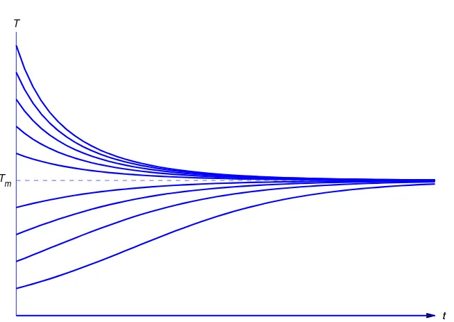
whereT0is the temperature of the body whent= 0. Thereforelimt→∞T(t) =Tm, independent ofT0. (Common sense suggests this. Why?)

Figure1.1.2shows typical graphs ofTversustfor various values ofT0.

Assuming that the medium remains at constant temperature seems reasonable if we’re considering a cup of coffee cooling in a room, but not if we’re cooling a huge cauldron of molten metal in the same room. The difference between the two situations is that the heat lost by the coffee isn’t likely to raise the temperature of the room appreciably, but the heat lost by the cooling metal is. In this second situation we must use a model that accounts for the heat exchanged between the object and the medium. LetT=T(t)

andTm = Tm(t)be the temperatures of the object and the medium respectively, and letT0andTm0 be their initial values. Again, we assume thatT andTmare related by (1.1.5). We also assume that the change in heat of the object as its temperature changes fromT0toT isa(T−T0)and the change in heat of the medium as its temperature changes fromTm0toTmisam(Tm−Tm0), whereaandamare positive constants depending upon the masses and thermal properties of the object and medium respectively. If we assume that the total heat of the in the object and the medium remains constant (that is, energy is conserved), then

a(T−T0) +am(Tm−Tm0) = 0.

Solving this forTmand substituting the result into (1.1.6) yields the differential equation

T0₌

−k

1 + a

am

T+k

Tm0+ a am

T0

for the temperature of the object. After learning to solve linear first order equations, you’ll be able to show (Exercise 4.2.17) that

T =aT0+amTm0

a+am

+am(T0−Tm0)

a+am

(14)

Section 1.1 Applications Leading to Differential Equations 5

T

t t T

[image:14.612.147.474.98.330.2]

m

Figure 1.1.2 Temperature according to Newton’s Law of Cooling

Glucose Absorption by the Body

Glucose is absorbed by the body at a rate proportional to the amount of glucose present in the bloodstream. Let λdenote the (positive) constant of proportionality. Suppose there areG0 units of glucose in the bloodstream whent = 0, and letG = G(t)be the number of units in the bloodstream at timet > 0. Then, since the glucose being absorbed by the body is leaving the bloodstream,Gsatisfies the equation

G0 ₌

−λG. (1.1.7)

From calculus you know that ifcis any constant then

G=ce−λt

(1.1.8)

satisfies (1.1.7), so (1.1.7) has infinitely many solutions. Settingt = 0 in (1.1.8) and requiring that G(0) =G0yieldsc=G0, so

G(t) =G0e−λt_.

Now let’s complicate matters by injecting glucose intravenously at a constant rate ofrunits of glucose per unit of time. Then the rate of change of the amount of glucose in the bloodstream per unit time is

G0₌

−λG+r, (1.1.9)

where the first term on the right is due to the absorption of the glucose by the body and the second term is due to the injection. After you’ve studied Section 2.1, you’ll be able to show (Exercise 2.1.43) that the solution of (1.1.9) that satisfiesG(0) =G0is

G= r

λ+

(15)

Graphs of this function are similar to those in Figure1.1.2. (Why?) Spread of Epidemics

One model for the spread of epidemics assumes that the number of people infected changes at a rate proportional to the product of the number of people already infected and the number of people who are susceptible, but not yet infected. Therefore, ifS denotes the total population of susceptible people and I = I(t)denotes the number of infected people at timet, thenS−Iis the number of people who are susceptible, but not yet infected. Thus,

I0₌_rI₍_S

−I),

whereris a positive constant. Assuming thatI(0) =I0, the solution of this equation is

I= SI0

I0+ (S−I0)e−rSt

(Exercise 2.2.29). Graphs of this function are similar to those in Figure1.1.1. (Why?) Sincelimt→∞I(t) =

S, this model predicts that all the susceptible people eventually become infected.

Newton’s Second Law of Motion

According toNewton’s second law of motion, the instantaneous accelerationaof an object with con-stant massmis related to the forceFacting on the object by the equationF=ma. For simplicity, let’s assume thatm= 1and the motion of the object is along a vertical line. Letybe the displacement of the object from some reference point on Earth’s surface, measured positive upward. In many applications, there are three kinds of forces that may act on the object:

(a) A force such as gravity that depends only on the position y, which we write as −p(y), where p(y)>0ify≥0.

(b) A force such as atmospheric resistance that depends on the position and velocity of the object, which we write as−q(y, y0₎_y0_{, where}_q_{is a nonnegative function and we’ve put}_y0 _{“outside” to indicate}

that the resistive force is always in the direction opposite to the velocity.

(c) A forcef =f(t), exerted from an external source (such as a towline from a helicopter) that depends only ont.

In this case, Newton’s second law implies that

y00₌

−q(y, y0₎_y0

−p(y) +f(t),

which is usually rewritten as

y00₊_q₍_{y, y}0₎_y0₊_p₍_y_{) =}_f₍_t₎_.

Since the second (and no higher) order derivative ofyoccurs in this equation, we say that it is asecond order differential equation.

Interacting Species: Competition

LetP =P(t)andQ=Q(t)be the populations of two species at timet, and assume that each population would grow exponentially if the other didn’t exist; that is, in the absence of competition we would have

P0₌_aP

and Q0₌_bQ,

(1.1.10)

wherea andb are positive constants. One way to model the effect of competition is to assume that the growth rate per individual of each population is reduced by an amount proportional to the other population, so (1.1.10) is replaced by

P0 ₌ _aP

−αQ Q0 ₌

(16)

Section 1.2Basic Concepts 7

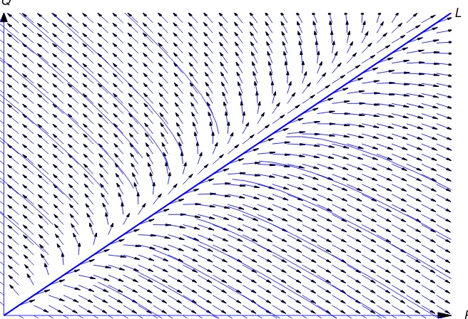
whereαandβare positive constants. (Since negative population doesn’t make sense, this system works only whileP andQare both positive.) Now supposeP(0) = P0 > 0 andQ(0) = Q0 > 0. It can be shown (Exercise 10.4.42) that there’s a positive constantρsuch that if (P0, Q0)is above the lineL through the origin with slopeρ, then the species with populationP becomes extinct in finite time, but if

(P0, Q0)is belowL, the species with populationQbecomes extinct in finite time. Figure1.1.3illustrates this. The curves shown there are given parametrically by P = P(t), Q = Q(t), t > 0. The arrows indicate direction along the curves with increasingt.

P Q

[image:16.612.144.472.207.431.2]

L

Figure 1.1.3 Populations of competing species

1.2 BASIC CONCEPTS

A differential equationis an equation that contains one or more derivatives of an unknown function.

Theorder of a differential equation is the order of the highest derivative that it contains. A differential equation is anordinary differential equationif it involves an unknown function of only one variable, or a

partial differential equationif it involves partial derivatives of a function of more than one variable. For now we’ll consider only ordinary differential equations, and we’ll just call themdifferential equations.

Throughout this text, all variables and constants are real unless it’s stated otherwise. We’ll usually use xfor the independent variable unless the independent variable is time; then we’ll uset.

The simplest differential equations are first order equations of the form

dy

dx =f(x) or, equivalently, y

0₌_f₍_x₎_,

wherefis a known function ofx. We already know from calculus how to find functions that satisfy this kind of equation. For example, if

(17)

then

y=

Z

x3dx=x

4

4 +c,

wherecis an arbitrary constant. Ifn >1we can find functionsythat satisfy equations of the form

y(n)₌_f₍_x₎ _(1.2.1)

by repeated integration. Again, this is a calculus problem.

Except for illustrative purposes in this section, there’s no need to consider differential equations like (1.2.1).We’ll usually consider differential equations that can be written as

y(n)=f(x, y, y0_{, . . . , y}(n−1)₎_, _(1.2.2)

where at least one of the functionsy,y0_{, . . . ,}_y(n−1)_{actually appears on the right. Here are some} exam-ples:

dy dx −x

2 ₌ ₀ _{(first order),}

dy dx+ 2xy

2 ₌

−2 (first order), d2y

dx2+ 2 dy

dx+y = 2x (second order), xy000₊_y2 ₌ _sin_x _{(third order),}

y(n)₊_xy0_{+ 3}_y ₌ _x _{(n-th order).}

Although none of these equations is written as in (1.2.2), all of themcanbe written in this form:

y0 ₌ _x2_,

y0 ₌ ₋₂₋₂_xy2_, y00 ₌ ₂_x₋₂_y0₋_y,

y000 ₌ sinx−y

2

x ,

y(n) ₌ _x₋_xy0₋₃_y.

Solutions of Differential Equations

Asolutionof a differential equation is a function that satisfies the differential equation on some open interval; thus,yis a solution of (1.2.2) ifyisntimes differentiable and

y(n)(x) =f(x, y(x), y0₍_x₎_{, . . . , y}(n−1)₍_x₎₎

for allxin some open interval(a, b). In this case, we also say thatyis a solution of(1.2.2)on(a, b). Functions that satisfy a differential equation at isolated points are not interesting. For example,y =x2 satisfies

xy0+x2= 3x

if and only ifx= 0orx= 1, but it’s not a solution of this differential equation because it does not satisfy the equation on an open interval.

(18)

Example 1.2.1 Ifais any positive constant, the circle

x2+y2=a2 (1.2.3)

is an integral curve of

y0 ₌

−x

y. (1.2.4)

To see this, note that the only functions whose graphs are segments of (1.2.3) are

y1=pa2₋_x2 _and _y2₌₋p_a2₋_x2_.

We leave it to you to verify that these functions both satisfy (1.2.4) on the open interval(−a, a). However, (1.2.3) is not a solution curve of (1.2.4), since it’s not the graph of a function.

Example 1.2.2 Verify that

y= x

2

3 + 1

x (1.2.5)

is a solution of

xy0₊_y₌_x2

(1.2.6)

on(0,∞)and on(−∞,0).

Solution Substituting (1.2.5) and

y0₌ 2x 3 −

1

x2 into (1.2.6) yields

xy0₍_x_{) +}_y₍_x_{) =}_x

2x

3 − 1

x2

+

x2

3 + 1

x

=x2

for allx6= 0. Thereforeyis a solution of (1.2.6) on(−∞,0)and(0,∞). However,yisn’t a solution of the differential equation on any open interval that containsx= 0, sinceyis not defined atx= 0.

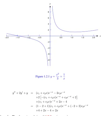
Figure1.2.1shows the graph of (1.2.5). The part of the graph of (1.2.5) on(0,∞)is a solution curve of (1.2.6), as is the part of the graph on(−∞,0).

Example 1.2.3 Show that ifc1andc2are constants then

y = (c1+c2x)e−x+ 2x−4 (1.2.7)

is a solution of

y00_{+ 2}_y0₊_y_{= 2}_x

(1.2.8)

on(−∞,∞).

Solution Differentiating (1.2.7) twice yields y0₌

−(c1+c2x)e−x₊_c2e−x_{+ 2}

and

y00_{= (}_c1₊_c2x₎_e−x

(19)

x y

0.5 1.0 1.5 2.0

−0.5 −1.0

−1.5 −2.0

2 4 6 8

−2

−4 −6

[image:19.612.122.470.105.503.2]

−8

Figure 1.2.1y= x 2

3 +

1

x

so

y00_{+ 2}_y0₊_y ₌ ₍_c1₊_c2x₎_e−x

−2c2e−x

+2

−(c1+c2x)e−x+c2e−x+ 2

+(c1+c2x)e−x_{+ 2}_x

−4

= (1−2 + 1)(c1+c2x)e−x+ (−2 + 2)c2e−x

+4 + 2x−4 = 2x

for all values ofx. Thereforeyis a solution of (1.2.8) on(−∞,∞).

Example 1.2.4 Find all solutions of

y(n)=e2x. (1.2.9)

Solution Integrating (1.2.9) yields

y(n−1)₌e2x

2 +k1,

wherek1is a constant. Ifn≥2, integrating again yields

y(n−2)₌ e2x

4 +k1x+k2.

Ifn≥3, repeatedly integrating yields

y= e

2x

2n +k1 xn−1

(n−1)! +k2

xn−2

(20)

wherek1,k2, . . . , knare constants. This shows that every solution of (1.2.9) has the form (1.2.10) for some choice of the constantsk1,k2, . . . ,kn. On the other hand, differentiating (1.2.10)ntimes shows that ifk1,k2, . . . ,knare arbitrary constants, then the functionyin (1.2.10) satisfies (1.2.9).

Since the constantsk1,k2, . . . ,knin (1.2.10) are arbitrary, so are the constants

k1

(n−1)!,

k2

(n−2)!,· · ·, kn.

Therefore Example1.2.4actually shows that all solutions of (1.2.9) can be written as

y=e

2x

2n +c1+c2x+· · ·+cnx n−1_,

where we renamed the arbitrary constants in (1.2.10) to obtain a simpler formula. As a general rule, arbitrary constants appearing in solutions of differential equations should be simplified if possible. You’ll see examples of this throughout the text.

Initial Value Problems

In Example1.2.4we saw that the differential equationy(n)₌_e2x_{has an infinite family of solutions that} depend upon thenarbitrary constantsc1,c2, . . . ,cn. In the absence of additional conditions, there’s no reason to prefer one solution of a differential equation over another. However, we’ll often be interested in finding a solution of a differential equation that satisfies one or more specific conditions. The next example illustrates this.

Example 1.2.5 Find a solution of

y0₌_x3

such thaty(1) = 2.

Solution At the beginning of this section we saw that the solutions ofy0 ₌_x3_are

y= x

4

4 +c.

To determine a value ofcsuch thaty(1) = 2, we setx= 1andy= 2here to obtain

2 =y(1) = 1

4 +c, so c= 7 4.

Therefore the required solution is

y =x

4_{+ 7}

4 .

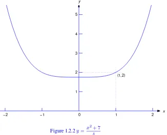
Figure1.2.2shows the graph of this solution. Note that imposing the conditiony(1) = 2is equivalent to requiring the graph ofyto pass through the point(1,2).

We can rewrite the problem considered in Example1.2.5more briefly as

y0=x3, y(1) = 2.

We call this an initial value problem. The requirementy(1) = 2is aninitial condition. Initial value problems can also be posed for higher order differential equations. For example,

y00

−2y0_{+ 3}_y₌_ex_, _y_{(0) = 1}_, _y0_{(0) = 2}

(21)

is an initial value problem for a second order differential equation wherey andy0 _{are required to have}

specified values atx = 0. In general, an initial value problem for an n-th order differential equation requiresyand its firstn−1derivatives to have specified values at some pointx0. These requirements are theinitial conditions.

1 2 3 4 5

0 1 2

−1 −2

(1,2)

[image:21.612.148.474.169.433.2]

x y

Figure 1.2.2y=x 2_{+ 7}

4

We’ll denote an initial value problem for a differential equation by writing the initial conditions after the equation, as in (1.2.11). For example, we would write an initial value problem for (1.2.2) as

y(n)=f(x, y, y0_{, . . . , y}(n−1)₎_{, y}₍_x0_{) =}_{k0, y}0₍_x0_{) =}_{k1, . . . , y}(n−1)₌_k

n−1. (1.2.12)

Consistent with our earlier definition of a solution of the differential equation in (1.2.12), we say thatyis a solution of the initial value problem (1.2.12) ifyisntimes differentiable and

y(n)(x) =f(x, y(x), y0(x), . . . , y(n−1)(x))

for allxin some open interval(a, b)that containsx0, andysatisfies the initial conditions in (1.2.12). The largest open interval that containsx0on whichy is defined and satisfies the differential equation is the

interval of validityofy.

Example 1.2.6 In Example1.2.5we saw that

y= x

4_{+ 7}

4 (1.2.13)

is a solution of the initial value problem

y0₌_x3_, _y_{(1) = 2}_.

(22)

Example 1.2.7 In Example1.2.2we verified that

y= x

2

3 + 1

x (1.2.14)

is a solution of

xy0₊_y₌_x2

on(0,∞)and on(−∞,0). By evaluating (1.2.14) atx=±1, you can see that (1.2.14) is a solution of the initial value problems

xy0₊_y₌_x2_, _y_{(1) =} 4

3 (1.2.15)

and

xy0+y=x2, y(−1) =−2₃. (1.2.16)

The interval of validity of (1.2.14) as a solution of (1.2.15) is(0,∞), since this is the largest interval that containsx0= 1on which (1.2.14) is defined. Similarly, the interval of validity of (1.2.14) as a solution of (1.2.16) is(−∞,0), since this is the largest interval that containsx0=−1on which (1.2.14) is defined.

Free Fall Under Constant Gravity

The term initial value problemoriginated in problems of motion where the independent variable is t (representing elapsed time), and the initial conditions are the position and velocity of an object at the initial (starting) time of an experiment.

Example 1.2.8 An object falls under the influence of gravity near Earth’s surface, where it can be as-sumed that the magnitude of the acceleration due to gravity is a constantg.

(a) Construct a mathematical model for the motion of the object in the form of an initial value problem for a second order differential equation, assuming that the altitude and velocity of the object at time t= 0are known. Assume that gravity is the only force acting on the object.

(b) Solve the initial value problem derived in(a)to obtain the altitude as a function of time.

SOLUTION(a) Lety(t)be the altitude of the object at timet. Since the acceleration of the object has

constant magnitudegand is in the downward (negative) direction,ysatisfies the second order equation

y00₌

−g,

where the prime now indicates differentiation with respect tot. Ify0 and v0 denote the altitude and velocity whent= 0, thenyis a solution of the initial value problem

y00₌

−g, y(0) =y0, y0_{(0) =}_v0.

(1.2.17)

SOLUTION(b) Integrating (1.2.17) twice yields

y0 ₌

−gt+c1,

y = −gt

2

2 +c1t+c2.

Imposing the initial conditionsy(0) =y0andy0_{(0) =}_v0_{in these two equations shows that}_c1₌_v0_and

c2=y0. Therefore the solution of the initial value problem (1.2.17) is

y=−gt

2

(23)

1.2 Exercises

1. Find the order of the equation. (a)d

2_y

dx2 + 2 dy dx

d3_y

dx3 +x= 0 (b)y

00

−3y0_{+ 2}_y₌_x7

(c)y0₋_y7_{= 0} _(d)_y00_y₋₍_y0₎2_{= 2}

2. Verify that the function is a solution of the differential equation on some interval, for any choice of the arbitrary constants appearing in the function.

(a) y=ce2x_; _y0_{= 2}_y

(b) y=x

2

3 +

c x; xy

0₊_y₌_x2

(c) y=1 2 +ce

−x2

; y0_{+ 2}_xy₌_x

(d) y= (1 +ce−x2

/2_{); (1}₋_ce−x2

/2₎−1 ₂_y0₊_x₍_y2₋_{1) = 0}

(e) y= tan

x3

3 +c

; y0 ₌_x2_{(1 +}_y2₎

(f) y= (c1+c2x)ex_{+ sin}_x₊_x2_; _y00₋₂_y0₊_y₌₋_{2 cos}_x₊_x2₋₄_x_{+ 2} (g) y=c1ex₊_c2x₊2

x; (1−x)y

00₊_xy0

−y= 4(1−x−x2₎_x−3

(h) y=x−1/2₍_c1_sin_x₊_c2_cos_x_{) + 4}_x_{+ 8}_; x2_y00₊_xy0₊

x2−1₄

y= 4x3+ 8x2+ 3x−2

3. Find all solutions of the equation.

(a) y0 ₌₋_x _(b) _y0₌₋_x_sin_x

(c) y0 ₌_x_ln_x _(d) _y00₌_x_cos_x

(e) y00_{= 2}_xex _(f) _y00_{= 2}_x_{+ sin}_x₊_ex (g) y000₌₋_cos_x _(h) _y000₌₋_x2₊_ex (i) y000_{= 7}_e4x

4. Solve the initial value problem. (a) y0 ₌₋_xex_, _y_{(0) = 1} (b) y0 ₌_x_sin_x2_, _y

r

π

2

= 1

(c) y0 _{= tan}_x, _y₍_π/_{4) = 3}

(d) y00₌_x4_, _y_{(2) =}₋₁_, _y0_{(2) =}₋₁

(e) y00₌_xe2x_, _y_{(0) = 7}_, _y0_{(0) = 1}

(f) y00₌₋_x_sin_x, _y_{(0) = 1}_, _y0_{(0) =}₋₃

(g) y000₌_x2_ex_, _y_{(0) = 1}_, _y0_{(0) =}

−2, y00_{(0) = 3}

(h) y000_{= 2 + sin 2}_x, _y_{(0) = 1}_, _y0_{(0) =}₋₆_, _y00_{(0) = 3}

(i) y000_{= 2}_x_{+ 1}_, _y_{(2) = 1}_, _y0_{(2) =}₋₄_, _y00_{(2) = 7}

5. Verify that the function is a solution of the initial value problem. (a) y=xcosx; y0 _{= cos}_x₋_y_tan_x, _y₍_π/_{4) =} π

4√2

(b) y=1 + 2 lnx

x2 +

1 2; y

0 ₌x2−2x2y+ 2

x3 , y(1) =

(24)

(c) y= tan

x2

2

; y0₌_x_{(1 +}_y2₎_, _y_{(0) = 0}

(d) y= 2

x−2; y

0₌ −y(y+ 1)

x , y(1) =−2

6. Verify that the function is a solution of the initial value problem. (a) y=x2_{(1 + ln}_x_); _y00₌ 3xy

0₋₄_y

x2 , y(e) = 2e

2_, _y0₍_e_{) = 5}_e

(b) y=x

2

3 +x−1; y

00₌ x2−xy

0₊_y_{+ 1}

x2 , y(1) =

1 3, y

0_{(1) =} 5 3

(c) y= (1 +x2₎−1/2_; _y00 ₌(x

2₋₁₎_y₋_x₍_x2_{+ 1)}_y0

(x2_{+ 1)}2 , y(0) = 1, y0_{(0) = 0}

(d) y= x

2

1−x; y

00

=2(x+y)(xy 0₋_y₎

x3 , y(1/2) = 1/2, y

0

(1/2) = 3

7. Suppose an object is launched from a point 320 feet above the earth with an initial velocity of 128 ft/sec upward, and the only force acting on it thereafter is gravity. Takeg= 32ft/sec2.

(a) Find the highest altitude attained by the object.

(b) Determine how long it takes for the object to fall to the ground. 8. Letabe a nonzero real number.

(a) Verify that ifcis an arbitrary constant then

y= (x−c)a (A)

is a solution of

y0 ₌_ay(a−1)/a _(B)

on(c,∞).

(b) Supposea <0ora >1. Can you think of a solution of (B) that isn’t of the form (A)? 9. Verify that

y=

(

ex₋₁_, _x_≥₀_,

1−e−x_{, x <}₀_, is a solution of

y0 ₌

|y|+ 1

on(−∞,∞). HINT:Use the definition of derivative atx= 0.

10. (a) Verify that ifcis any real number then

y=c2+cx+ 2c+ 1 (A)

satisfies

y0₌ −(x+ 2) +

p

x2_{+ 4}_x_{+ 4}_y

2 (B)

on some open interval. Identify the open interval. (b) Verify that

y1= −x(x+ 4) 4

(25)

1.3 DIRECTION FIELDS FOR FIRST ORDER EQUATIONS

It’s impossible to find explicit formulas for solutions of some differential equations. Even if there are such formulas, they may be so complicated that they’re useless. In this case we may resort to graphical or numerical methods to get some idea of how the solutions of the given equation behave.

In Section 2.3 we’ll take up the question of existence of solutions of a first order equation

y0 ₌_f₍_{x, y}₎_.

(1.3.1)

In this section we’ll simply assume that (1.3.1) has solutions and discuss a graphical method for ap-proximating them. In Chapter 3 we discuss numerical methods for obtaining approximate solutions of (1.3.1).

Recall that a solution of (1.3.1) is a functiony=y(x)such that

y0₍_x_{) =}_f₍_{x, y}₍_x₎₎

for all values ofxin some interval, and an integral curve is either the graph of a solution or is made up of segments that are graphs of solutions. Therefore, not being able to solve (1.3.1) is equivalent to not knowing the equations of integral curves of (1.3.1). However, it’s easy to calculate the slopes of these curves. To be specific, the slope of an integral curve of (1.3.1) through a given point(x0, y0)is given by the numberf(x0, y0). This is the basis ofthe method of direction fields.

Iff is defined on a setR, we can construct adirection field for (1.3.1) inRby drawing a short line segment through each point(x, y)inRwith slopef(x, y). Of course, as a practical matter, we can’t actually draw line segments througheverypoint inR; rather, we must select a finite set of points inR. For example, supposef is defined on the closed rectangular region

R:{a≤x≤b, c≤y ≤d}.

Let

a=x0< x1<· · ·< xm=b

be equally spaced points in[a, b]and

c=y0< y1<· · ·< yn =d

be equally spaced points in[c, d]. We say that the points

(xi, yj), 0≤i≤m, 0≤j ≤n,

(26)

Section 1.3Direction Fields for First Order Equations 17

y

x a b c

d

Figure 1.3.1 A rectangular grid

Unfortunately, approximating a direction field and graphing integral curves in this way is too tedious to be done effectively by hand. However, there is software for doing this. As you’ll see, the combina-tion of direccombina-tion fields and integral curves gives useful insights into the behavior of the solucombina-tions of the differential equation even if we can’t obtain exact solutions.

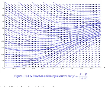
We’ll study numerical methods for solving a single first order equation (1.3.1) in Chapter 3. These methods can be used to plot solution curves of (1.3.1) in a rectangular regionRiff is continuous onR. Figures1.3.2,1.3.3, and1.3.4show direction fields and solution curves for the differential equations

y0 = x

2₋_y2

1 +x2₊_y2, y

0

= 1 +xy2, and y0= x−y 1 +x2,

which are all of the form (1.3.1) withf continuous for all(x, y).

−4 −3 −2 −1 0 1 2 3 4

y

x

Figure 1.3.2 A direction field and integral curves

fory= x 2₋_y2 1 +x2₊_y2

−2 −1.5 −1 −0.5 0 0.5 1 1.5 2

−2 −1.5 −1 −0.5 0 0.5 1 1.5 2 y

x

Figure 1.3.3 A direction field and integral curves for

(27)

−1 −0.8 −0.6 −0.4 −0.2 0 0.2 0.4 0.6 0.8 1 −1

−0.8 −0.6 −0.4 −0.2 0 0.2 0.4 0.6 0.8 1

y

[image:27.612.128.480.114.401.2]

x

Figure 1.3.4 A direction and integral curves fory0₌ x−y

1 +x2

The methods of Chapter 3 won’t work for the equation

y0₌

−x/y (1.3.2)

ifRcontains part of thex-axis, sincef(x, y) =−x/yis undefined wheny = 0. Similarly, they won’t work for the equation

y0₌ x2

1−x2₋_y2 (1.3.3)

ifR contains any part of the unit circlex2₊_y2 _{= 1}_{, because the right side of (1.3.3) is undefined if} x2₊_y2_{= 1}_{. However, (1.3.2) and (1.3.3) can written as}

y0 ₌ A(x, y)

B(x, y) (1.3.4)

whereAandB are continuous on any rectangleR. Because of this, some differential equation software is based on numerically solving pairs of equations of the form

dx

dt =B(x, y), dy

dt =A(x, y) (1.3.5)

wherexandyare regarded as functions of a parametert. Ifx=x(t)andy=y(t)satisfy these equations, then

y0 ₌ dy

dx = dy dt

dx dt =

A(x, y)

B(x, y),

(28)

Eqns. (1.3.2) and (1.3.3) can be reformulated as in (1.3.4) with

dx dt =−y,

dy dt =x

and

dx

dt = 1−x 2

−y2, dy dt =x

2_,

respectively. Even iff is continuous and otherwise “nice” throughoutR, your software may require you to reformulate the equationy0 ₌_f₍_{x, y}₎_as

dx dt = 1,

dy

dt =f(x, y),

which is of the form (1.3.5) withA(x, y) =f(x, y)andB(x, y) = 1.

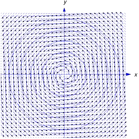
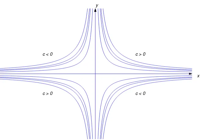
Figure1.3.5shows a direction field and some integral curves for (1.3.2). As we saw in Example1.2.1 and will verify again in Section 2.2, the integral curves of (1.3.2) are circles centered at the origin.

[image:28.612.193.423.303.533.2]

x y

Figure 1.3.5 A direction field and integral curves fory0 ₌₋x

y

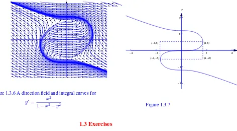
Figure1.3.6shows a direction field and some integral curves for (1.3.3). The integral curves near the top and bottom are solution curves. However, the integral curves near the middle are more complicated. For example, Figure1.3.7shows the integral curve through the origin. The vertices of the dashed rectangle are on the circlex2₊_y2 _{= 1}_(a _≈ _.₈₄₆_,_b _≈ _.₅₃₃_{), where all integral curves of (1.3.3) have infinite} slope. There are three solution curves of (1.3.3) on the integral curve in the figure: the segment above the levely=bis the graph of a solution on(−∞, a), the segment below the levely=−bis the graph of a solution on(−a,∞), and the segment between these two levels is the graph of a solution on(−a, a).

(29)

As you study from this book, you’ll often be asked to use computer software and graphics. Exercises with this intent are marked as C (computer or calculator required), C/G (computer and/or graphics required), or L (laboratory work requiring software and/or graphics). Often you may not completely understand how the software does what it does. This is similar to the situation most people are in when they drive automobiles or watch television, and it doesn’t decrease the value of using modern technology as an aid to learning. Just be careful that you use the technology as a supplement to thought rather than a substitute for it.

y

[image:29.612.105.577.209.469.2]

x

Figure 1.3.6 A direction field and integral curves for

y0 ₌ x 2

1−x2₋_y2

x y

(a,−b) (a,b) (−a,b)

(−a,−b)

1 2

−1 −2

1 2

−1

−2

Figure 1.3.7

1.3 Exercises

(30)

−1 −0.8 −0.6 −0.4 −0.2 0 0.2 0.4 0.6 0.8 1

x y

1 A direction field fory0 ₌ x

(31)

0 0.5 1 1.5 2 2.5 3 3.5 4 −2

−1.5 −1 −0.5 0 0.5 1 1.5 2

x y

2 A direction field fory0 ₌ 2xy2

1 +x2

0 0.2 0.4 0.6 0.8 1 1.2 1.4 1.6 1.8 2

−1 −0.8 −0.6 −0.4 −0.2 0 0.2 0.4 0.6 0.8 1

x y

(32)

0 0.2 0.4 0.6 0.8 1 1.2 1.4 1.6 1.8 2

−1 −0.8 −0.6 −0.4 −0.2 0 0.2 0.4 0.6 0.8 1

x y

4 A direction field fory0 ₌ 1

1 +x2₊_y2

0 0.5 1 1.5 2 2.5 3

−1 −0.8 −0.6 −0.4 −0.2 0 0.2 0.4 0.6 0.8 1

x y

5 A direction field fory0 ₌

(33)

−1 −0.8 −0.6 −0.4 −0.2 0 0.2 0.4 0.6 0.8 1 −1

−0.8 −0.6 −0.4 −0.2 0 0.2 0.4 0.6 0.8 1

x y

6 A direction field fory0 _{= (}_x2₊_y2₎1/2

0 1 2 3 4 5 6 7

−3 −2 −1 0 1 2 3

x y

(34)

0 0.1 0.2 0.3 0.4 0.5 0.6 0.7 0.8 0.9 1

x y

8 A direction field fory0 ₌_exy

0 0.2 0.4 0.6 0.8 1 1.2 1.4 1.6 1.8 2

−1 −0.8 −0.6 −0.4 −0.2 0 0.2 0.4 0.6 0.8 1

x y

9 A direction field fory0 _{= (}_x

(35)

1 1.2 1.4 1.6 1.8 2 2.2 2.4 2.6 2.8 3 −1

−0.8 −0.6 −0.4 −0.2 0 0.2 0.4 0.6 0.8 1

x y

10 A direction field fory0₌_x3_y2₊_xy3

0 0.5 1 1.5 2 2.5 3 3.5 4

x y

(36)

In Exercises12-22construct a direction field and plot some integral curves in the indicated rectangular region.

12. C/G y0₌_y₍_y₋_1); _{−₁_≤_x_≤₂_, ₋₂_≤_y_≤₂_}

13. C/G y0_{= 2}

−3xy; {−1≤x≤4, −4≤y≤4}

14. C/G y0₌_xy₍_y₋_1); _{−₂_≤_x_≤₂_, ₋₄_≤_y_≤₄_}

15. C/G y0_{= 3}_x₊_y_; _{−₂_≤_x_≤₂_, ₀_≤_y_≤₄_}

16. C/G y0₌_y₋_x3_; _{−₂_≤_x_≤₂_, ₋₂_≤_y_≤₂_} 17. C/G y0_{= 1}₋_x2₋_y2_; _{−₂_≤_x_≤₂_, ₋₂_≤_y _≤₂_} 18. C/G y0₌_x₍_y2₋_1); _{−₃_≤_x_≤₃_, ₋₃_≤_y_≤₂_}

19. C/G y0₌ x

y(y2₋₁₎; {−2≤x≤2, −2≤y≤2}

20. C/G y0₌ xy

2

y−1; {−2≤x≤2, −1≤y≤4}

21. C/G y0₌ x(y

2₋₁₎

y ; {−1≤x≤1, −2≤y≤2}

22. C/G y0₌₋ x

2₊_y2

1−x2₋_y2; {−2≤x≤2, −2≤y≤2}

23. L By suitably renaming the constants and dependent variables in the equations T0₌

−k(T −Tm) (A)

and

G0₌

−λG+r (B)

discussed in Section 1.2 in connection with Newton’s law of cooling and absorption of glucose in the body, we can write both as

y0 ₌

−ay+b, (C)

whereais a positive constant andbis an arbitrary constant. Thus, (A) is of the form (C) with y =T,a =k, andb =kTm, and (B) is of the form (C) withy =G,a=λ, andb =r. We’ll encounter equations of the form (C) in many other applications in Chapter 2.

Choose a positiveaand an arbitraryb. Construct a direction field and plot some integral curves for (C) in a rectangular region of the form

{0≤t≤T, c≤y ≤d}

of thety-plane. VaryT,c, andduntil you discover a common property of all the solutions of (C). Repeat this experiment with various choices ofaandbuntil you can state this property precisely in terms ofaandb.

24. L By suitably renaming the constants and dependent variables in the equations P0 ₌_aP₍₁

−αP) (A)

and

I0₌_rI₍_S

(37)

discussed in Section 1.1 in connection with Verhulst’s population model and the spread of an epidemic, we can write both in the form

y0₌_ay

−by2, (C)

whereaandbare positive constants. Thus, (A) is of the form (C) withy=P,a=a, andb=aα, and (B) is of the form (C) withy=I,a=rS, andb=r. In Chapter 2 we’ll encounter equations of the form (C) in other applications..

(a) Choose positive numbersaandb. Construct a direction field and plot some integral curves for (C) in a rectangular region of the form

{0≤t≤T, 0≤y ≤d}

of thety-plane. VaryT andduntil you discover a common property of all solutions of (C) withy(0) >0. Repeat this experiment with various choices ofaandbuntil you can state this property precisely in terms ofaandb.

(b) Choose positive numbersaandb. Construct a direction field and plot some integral curves for (C) in a rectangular region of the form

{0≤t≤T, c≤y≤0}

of thety-plane. Varya,b,T andcuntil you discover a common property of all solutions of (C) withy(0)<0.

(38)

CHAPTER 2 First Order Equations

IN THIS CHAPTER we study first order equations for which there are general methods of solution.

SECTION 2.1 deals with linear equations, the simplest kind of first order equations. In this section we introduce the method of variation of parameters. The idea underlying this method will be a unifying theme for our approach to solving many different kinds of differential equations throughout the book.

SECTION 2.2 deals with separable equations, the simplest nonlinear equations. In this section we intro-duce the idea of implicit and constant solutions of differential equations, and we point out some differ-ences between the properties of linear and nonlinear equations.

SECTION 2.3 discusses existence and uniqueness of solutions of nonlinear equations. Although it may seem logical to place this section before Section 2.2, we presented Section 2.2 first so we could have illustrative examples in Section 2.3.

SECTION 2.4 deals with nonlinear equations that are not separable, but can be transformed into separable equations by a procedure similar to variation of parameters.

SECTION 2.5 covers exact differential equations, which are given this name because the method for solving them uses the idea of an exact differential from calculus.

SECTION 2.6 deals with equations that are not exact, but can made exact by multiplying them by a function known calledintegrating factor.

(39)

2.1 LINEAR FIRST ORDER EQUATIONS

A first order differential equation is said to belinearif it can be written as

y0₊_p₍_x₎_y₌_f₍_x₎_. _(2.1.1)

A first order differential equation that can’t be written like this is nonlinear. We say that (2.1.1) is

homogeneous iff ≡ 0; otherwise it’s nonhomogeneous. Sincey ≡ 0 is obviously a solution of the

homgeneous equation

y0+p(x)y= 0,

we call it thetrivial solution. Any other solution isnontrivial.

Example 2.1.1 The first order equations

x2_y0_{+ 3}_y ₌ _x2_,

xy0

−8x2y = sinx, xy0_{+ (ln}_x₎_y ₌ ₀_,

y0 ₌ _x2_y₋₂_,

are not in the form (2.1.1), but they are linear, since they can be rewritten as

y0₊ 3

x2y = 1,

y0

−8xy = sinx

x ,

y0₊lnx

x y = 0, y0

−x2y = −2.

Example 2.1.2 Here are some nonlinear first order equations:

xy0_{+ 3}_y2 _{= 2}_x _(because_y_{is squared),}

yy0 ₌ ₃ _{(because of the product}_yy0_),

y0₊_xey ₌ ₁₂ _{(because of}_ey_).

General Solution of a Linear First Order Equation

To motivate a definition that we’ll need, consider the simple linear first order equation

y0₌ 1

x2. (2.1.2)

From calculus we know thatysatisfies this equation if and only if

y=−1_x+c, (2.1.3)

(40)

Section 2.1Linear First Order Equations 31

(−∞,0)and(0,∞); moreover, every solution of (2.1.2) on either of these intervals is of the form (2.1.3) for some choice ofc. We say that (2.1.3) isthe general solutionof (2.1.2).

We’ll see that a similar situation occurs in connection with any first order linear equation

y0₊_p₍_x₎_y₌_f₍_x_); _(2.1.4)

that is, ifpandf are continuous on some open interval(a, b)then there’s a unique formulay =y(x, c)

analogous to (2.1.3) that involvesxand a parametercand has the these properties:

• For each fixed value ofc, the resulting function ofxis a solution of (2.1.4) on(a, b).

• Ify is a solution of (2.1.4) on (a, b), then y can be obtained from the formula by choosing c appropriately.

We’ll cally=y(x, c)thegeneral solutionof (2.1.4).

When this has been established, it will follow that an equation of the form

P0(x)y0₊_P1₍_x₎_y₌_F₍_x₎ _(2.1.5)

has a general solution on any open interval(a, b)on whichP0,P1, andF are all continuous andP0has no zeros, since in this case we can rewrite (2.1.5) in the form (2.1.4) withp=P1/P0andf =F/P0, which are both continuous on(a, b).

To avoid awkward wording in examples and exercises, we won’t specify the interval(a, b)when we ask for the general solution of a specific linear first order equation. Let’s agree that this always means that we want the general solution on every open interval on whichpandf are continuous if the equation is of the form (2.1.4), or on whichP0,P1, andFare continuous andP0has no zeros, if the equation is of the form (2.1.5). We leave it to you to identify these intervals in specific examples and exercises.

For completeness, we point out that ifP0,P1, andF are all continuous on an open interval(a, b), but P0doeshave a zero in(a, b), then (2.1.5) may fail to have a general solution on(a, b)in the sense just defined. Since this isn’t a major point that needs to be developed in depth, we won’t discuss it further; however, see Exercise44for an example.

Homogeneous Linear First Order Equations

We begin with the problem of finding the general solution of a homogeneous linear first order equation. The next example recalls a familiar result from calculus.

Example 2.1.3 Letabe a constant. (a) Find the general solution of

y0−ay= 0. (2.1.6)

(b) Solve the initial value problem y0

−ay= 0, y(x0) =y0.

SOLUTION(a) You already know from calculus that ifcis any constant, theny=ceax_{satisfies (2.1.6).}

However, let’s pretend you’ve forgotten this, and use this problem to illustrate a general method for solving a homogeneous linear first order equation.

We know that (2.1.6) has the trivial solutiony≡0. Now supposeyis a nontrivial solution of (2.1.6). Then, since a differentiable function must be continuous, there must be some open intervalIon whichy has no zeros. We rewrite (2.1.6) as

y0

(41)

x

0.2 0.4 0.6 0.8 1.0

y

0.5 1.0 1.5 2.0 2.5 3.0

a = 2

a = 1.5 a = 1

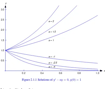
[image:41.612.129.469.103.393.2]

a = −1 a = −2.5 a = −4

Figure 2.1.1 Solutions ofy0

−ay= 0,y(0) = 1

forxinI. Integrating this shows that

ln|y|=ax+k, so _|y|=ekeax,

wherekis an arbitrary constant. Sinceeax _{can never equal zero,}_y_{has no zeros, so}_y _{is either always} positive or always negative. Therefore we can rewriteyas

y=ceax _(2.1.7)

where

c=

ek _if_{y >}₀_,

−ek _if_{y <}₀_.

This shows that every nontrivial solution of (2.1.6) is of the formy=ceax_{for some nonzero constant}_c. Since settingc= 0yields the trivial solution,allsolutions of (2.1.6) are of the form (2.1.7). Conversely, (2.1.7) is a solution of (2.1.6) for every choice ofc, since differentiating (2.1.7) yieldsy0₌_aceax ₌_ay.

SOLUTION(b) Imposing the initial conditiony(x0) =y0yieldsy0=ceax0_{, so}c=y0e−ax0_and

y=y0e−ax0_eax₌_y0ea(x−x0)_.

Figure2.1.1show the graphs of this function withx0= 0,y0= 1, and various values ofa.

Example 2.1.4 (a) Find the general solution of

xy0₊_y_{= 0}_. _(2.1.8)

(b) Solve the initial value problem