A Wavelet Network based Model for Ni-Cd Batteries

Int. J. Electrochem. Sci., 7 (2012) 10291 - 10302

International Journal of

ELECTROCHEMICAL

SCIENCE

A Wavelet Network based Model for Ni-Cd Batteries

Mohammad Sarvi*, Navid Ghaffarzadeh*

Technical and Engineering Faculty, Imam Khomeini International University, Qazvin, Iran

*

E-mail: [email protected], [email protected]

Received: 15 July 2012 / Accepted: 28 August 2012 / Published: 1 October 2012

Ni-Cd batteries are nonlinear electrochemical devices with different characteristics at different charge currents. This paper proposes a wavelet network based method for simulation and modeling of Ni-Cd batteries that considers the impact of charge current. It does not have the limitations associated with traditional neural networks or neuro-fuzzy-based algorithms such as convergence to local optimum points, over-fit and/or under-fit problems. Simulations and measurements are performed for the wavelet network and advantages of the model are presented. Inputs of the wavelet network are battery current (Ibat), no load voltage and time (t) while battery voltage (Vbat) is selected as the output. An

experimental setup is used to validate the accuracy of the model at different charge rates. Computed and measured results show good agreements for a 7AH, size F, Ni-Cd battery, manufactured by SANYO. Theoretical and experimental results are compared and analyzed.

Keywords: Battery, Modeling, Wavelet Network.

1. INTRODUCTION

Rechargeable batteries are widely used in many electrical systems to store and deliver energy. The most familiar applications are staring, lighting and ignition (SLI) automotive, industrial truck materials-handling equipment, as well as emergency and standby power [1].

The ultra-fast charging capability, fine performance and high capacity of Nickel Cadmium batteries along with their limited weight and size are attractive and distinct properties for light and compact equipment. Ni-Cd batteries have found many applications including cordless and portable equipment, photovoltaic systems, electric vehicle [2] satellites [3-4], and power plant supporting equipment [5-7].

of [2] are assumed to be independent of charging current. Therefore, this model is not accurate under varying battery current condition. The model parameters presented for Nickel-Hydrogen [9-10], Lithium-Ion [11] and Lead-Acid [2, 12-15] batteries depend on chemical reactions, which makes the simulation procedure very complicated. Most of these models ignore the nonlinear electrochemical characteristics of the battery and the variation of battery voltage during charge and discharge states. In addition, most of proposed models ignore the change of battery impedance with respect to charge current and assume constant model parameters at different charge and discharge states.

Neural networks have been used for power system applications [16-17]. They have the limitations and problems such as convergence to local optimum points, over-fit and/or under-fit problems which make them somewhat unreliable. Wavelet Networks (WNs) have better performances as compared with the traditional neural networks [18-20] and are implemented in this paper.

The subject of this paper is to introduce a WN model for Ni-Cd batteries and to investigate its accuracy through different measurements. The main contribution is nonlinear nature of model parameter and their dependency on battery charging current.

2. ELECTRICAL MODELS of Ni-Cd BATTERIES

Battery characteristics play a dominant role in the electrical power system (EPS) performance. Accurate battery models are essential for the simulation of EPS.

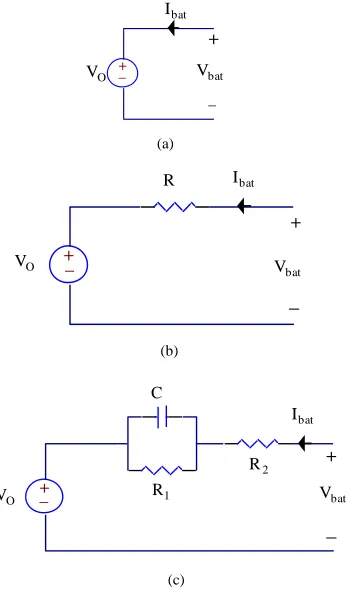
2.1. Ideal Model

The ideal equivalent model of the Ni-Cd battery consists of a simple voltage source [2], as shown in Fig. 1(a):

o bat t V

V ( ) (1)

This model does not reflect the physical characteristics of the battery since it’s nonlinear behavior and internal parameters are ignored.

2.2. Linear Model

The linear model of the Ni-Cd battery (Fig. 1 (b)) includes its internal resistance [2, 14-15]. Furthermore, voltage source V and internal resistance R are fixed and don't change with charge/discharge rates:

o bat

bat t RI V

2.3. Thevenin Model

The Thevenin model of Ni-Cd battery contains the electrical values of no-load voltage (V), internal resistance (R2) and a parallel R1Ccircuit that incorporates the impact of over voltage conditions [2-4], as shown in Fig. 1(c). The battery voltage can be computed as:

o C R

t

bat bat

bat t R I R I e V

V    



) 1

( )

( 1

1

2 (3)

Parameters of R1,R2,C and Vo are computed for a given charge current using measurements. These parameters are fixed and don't change with charge current. Therefore, this model is not accurate for other charge currents.

2.4. The Proposed Wavelet Network Model for Ni-Cd Batteries

The main limitation of previous models is the ignorance of nonlinear electrochemical behavior of battery. This causes nonlinear variation of parameters with respect to charging rates. The proposed model has the benefits and advantages of WNs such as high reliability and robustness against system failure. Furthermore, the nonlinear electro-chemical behaviors of batteries and their dependency on charging current has taken into consideration which makes the simulation results more accurate.

(b)

+_{_} O

V

bat

V R

+

_

bat

I

(c) +

_

_

O

V

C

1

R

2

R

bat

I

+

bat

V

(a)

+ _

+_{_}

+ _ O

V

bat

I

bat

V

+

_

3. WAVELET NETWORKS

Wavelet networks (WNs) belong to the class of feed forward neural networks, with wavelets as the activation functions [19]. Unlike the feed forward neural networks, the structure of WNs can be obtained based on wavelet theory. WNs are based on the wavelet transform, orthonormal wavelet and wavelet frames [20].

3.1. Discrete Wavelet Transform

The discrete wavelet transform (DWT) is the basic tool for the feature extraction. DWT is the discrete counterpart of the continuous wavelet transform (CWT). The CWT of a continuous time signal is defined as

 

 

 

CWT   *_a,b  



 

 (4)

with

 

      

a b t

a 1

t *

* b ,

a 

 (5)

where 

 

scaling (dilation) and translating parameters, respectively. The scale parameter a sets the oscillatory frequency and the length of the wavelet, while the translation parameter b deposits its shifting position. In a practical application, the DWT is used instead of the CWT. This is implemented by using discrete values aa₀m and bnb₀a₀m for the scaling parameter and translation parameter, respectively. Then

 





m

0 n ,

m   

 



 (6)

where m and n indicate frequency localization and time localization, respectively. Generally, we can choose a0=2 and b0=1 to provide a dyadic-orthonormal wavelet transform and the basis for multi-resolution analysis (MRA).

In MRA, signal f(t) is decomposed in terms of the approximations and details which are presented by scaling functions m,n

 

 

 





m

n ,

m   





 





m

n ,

m  

 



 (8)

The scaling function is associated with the low-pass filters (with filter coefficients {g0(n)}) and the wavelet function is associated with the high-pass filters (with filter coefficients {g1(n)}). The so-called two scale equations give rise to these filters [21].

 

 





n 0



 

 (9)

 

 





n 1



 

 (10)

Filter g1(n) is an alternating flip of filter g0(n) and there exists an odd integer N such that [22]

    



g₁   n ₀   (11)

The decomposition procedure starts with passing a signal through these filters. The approximation is the output of low-pass filter while the detail is the output of the high-pass filter.

3.2.Wavelet Frames and Orthonormal Wavelet

There are two classifications of wavelet functions [23]; orthonormal wavelet and wavelet frames. Construction of orthonormal WNs is complicated and they don’t benefit from the full advantages of orthonormal basis due to the sparseness of the training data. On the other hand, wavelet frames offer more freedom on the choice of the wavelet function. It is possible to generate a single-scaling frame of L2(Rd) with a single mother wavelet function. In contrast, in order to construct a single-scaling orthonormal wavelet basis of L2(Rd), 2d-1 mother wavelet functions and one scaling function are required. This complicates the analysis and augments the required computing times.

3.3. Wavelet Network Structure

To approximate an arbitrarily nonlinear function, there are two processes in the WN algorithm: network construction (e.g., using network structure to analyse the wavelet and updating its parameter to retain the network topology for further processing) and error minimisation (e.g., minimisation based on an adaptive Least Mean Square (LMS) algorithm and updating parameter of the network initialisation using the steepest-descent gradient method).

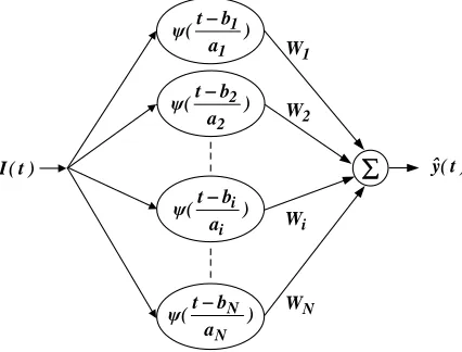
The WN architecture approximates a signal yˆ(t)with linear combination of a set of daughter

wavelet (Eq. 5) which is formed with dilation a and translation b of the mother wavelet [20]. The approximate signal of the network yˆ(t)can be written as

) ( . ). ( )

( ˆ

1 i

i N

i

i

a b t w t I t

y 





where N is the number of wavelet and wi is the weight coefficient. Fig. 2 depicts the structure of a WN.

 N W ) a b t ( ψ N N  ) a b t ( ψ i i  ) a b t ( ψ 1 1  ) a b t ( ψ 2 2  i W 2 W 1 W ) t ( y ˆ ) t ( I

Figure 2. Structure of a wavelet network.

Determination of the number of wavelet (N) is an important task to reduce the model order problem. To solve this problem, a part of the model data is used to approximate the model order. For this purpose, several approaches exist, such as cross-validation, generalised cross-validation, model complexity penalty, statistical hypothesis test, minimum description length criterion, Mallows criterion and Akaike Final Prediction Error (AFPE) [23]. In this paper, the AFPE approach is adopted and used to minimise the Equation:

 



AFPE ( fˆ (I ) y )

n 2 1 . N . 2 d . N n N . 2 d . N n fˆ

J (13)

where fˆ is the wavelet network, _s N is the number of wavelets in the network, d_I is the input dimension and n is the sample length of the training data.

The wavelet network parameters wi , bi and ai are optimised by using LMS to minimize the cost as a function of energy at time t, with

) t ( y ˆ ) t ( y ) t (

e   (14)

where y(t) is the expected output. The objective function is defined as:



E (15)

To minimise E, several methods such as conjugate gradients, Broyden-Fletcher-Goldfarb-Shanno (BFGS) and steepest descent exist. In this paper, the steepest descent method is applied, which requires the gradients

i i a E w E    

, and

i b E 

 _{to update the parameters w}

4. SIMULATION of Ni-Cd BATTERY

The ideal, linear, and Thevenin models of the Ni-Cd battery (Fig. 1) are simulated using SIMULINK facility of MATLAB. Also the wavelet network is trained using measurement data and a MATLAB subroutine is used for battery simulation. In order to simulate battery characteristics at different charge currents, the value of Ic is changed. It should be noted that the wavelet function  has

been chosen as:

x x x e

x d

x T

x

 

  2

2 2

, ) (

) (

2

 (16)

where is so-called "Mexican hat" and x 2  xTx

5. MEASURING ELECTRICAL CHARACTERISTICS of Ni-Cd BATTERY

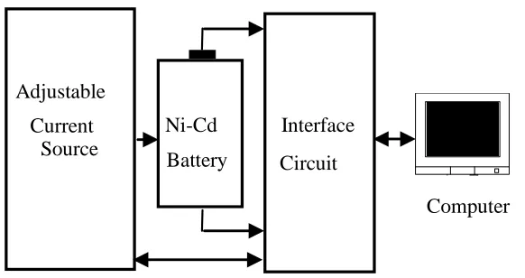
In order to train and validate the proposed wavelet network model and to investigate its accuracy, an experimental setup consisting of an adjustable current source, a personal computer, an interface board and a 7AH Ni-Cd battery is used as shown in Fig. 3.

The adjustable current source generates the desired current level for battery charging. The interface board samples battery voltage during charging time (about one hour) and stores data in the personal computer.

Battery

Current Ni-Cd Interface

Adjustable

Circuit Source

Computer

Figure 3. The experimental setup used to measure battery characteristics.

6. COMPARISON of SIMULATED and MEASURED RESULTS

Simulated and measured results are compared for different battery current levels. Comparisons of computed and measured results are presented for two reasons:

0 500 1000 1500 2000 2500

0.9 1 1.1 1.2 1.3 1.4 1.5 1.6 1.7 1.8

Battery current = 3.5 A

time (sec)

Bat

tery

v

o

lt

ag

e

(v

)

Figure 4. Comparison of simulated and measured battery voltages at charge current Ic=3.5 A; (1:

ideal model, 2: linear model, 3: Thevenin model, 4: proposed model, 5: measured characteristics).

0 500 1000 1500 2000 2500

0.9 1 1.1 1.2 1.3 1.4 1.5 1.6 1.7 1.8

time (sec)

Bat

tery

v

o

lt

ag

e

(v

)

Battery current = 4 A

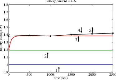
Figure 5. Comparison of simulated and measured battery voltages at charge current Ic=4 A; (1: ideal

model, 2: linear model, 3: Thevenin model, 4: proposed model, 5: measured characteristics).

1

2

3

4

5

1

2

3

0 500 1000 1500 2000 2500

0.9 1 1.1 1.2 1.3 1.4 1.5 1.6 1.7 1.8

Battery current = 5.25 A

time (sec)

Bat

tery

v

o

lt

ag

e

(v

)

Figure 6. Comparison of simulated and measured battery voltages at charge current Ic=5.25 A; (1:

ideal model, 2: linear model, 3: Thevenin model, 4: proposed model, 5: measured characteristics).

0 500 1000 1500 2000 2500

0.9 1 1.1 1.2 1.3 1.4 1.5 1.6 1.7 1.8

Battery current = 7 A

time (sec)

Bat

tery

v

o

lt

ag

e

(v

)

Figure 7. Comparison of simulated and measured battery voltages at charge current Ic=7 A; (1: ideal

model, 2: linear model, 3: Thevenin model, 4: proposed model, 5: measured characteristics).

1

2

4

5

3

1

2

4

5

0 500 1000 1500 2000 2500

0.9 1 1.1 1.2 1.3 1.4 1.5 1.6 1.7 1.8

Battery current = 5 A

time (sec)

Bat

tery

v

o

lt

ag

e

(v

)

Figure 8. Comparison of simulated and measured battery voltages at charge current Ic=5 A; (1: ideal

model, 2: linear model, 3: Thevenin model, 4: proposed model, 5: measured characteristics).

0 500 1000 1500 2000 2500

1 1.2 1.4 1.6 1.8

Battery current = 6 A

time (sec)

Bat

tery

v

o

lt

ag

e

(v

)

Figure 9. Comparison of simulated and measured battery voltages at charge current Ic=6 A; (1: ideal

model, 2: linear model, 3: Thevenin model, 4: proposed model, 5: measured characteristics).

1

2

3

5

4

1

2

4

5

A. To train the proposed wavelet network model at charge currents used for computing battery parameters (e.g., 3.5A, 4A, 5.25A and 7A) as shown in Figs. 4 to 7.

B. To investigate the accuracy of the model at other charge currents (e.g., 5A and 6A) as shown in Figs. 8 and 9.

Results show that the conventional models (e.g., ideal, linear, Thevenin) can not accurately predict battery characteristics (Figs. 4-9). On the other hand if the proposed wavelet network model is used, the computed and measured battery voltages show very good agreements for different levels of charge/discharge currents. Similar results were noticed at other charge currents.

7. CONCLUSION

A wavelet network model to simulate the behavior of Ni-Cd batteries is presented. Based on the computed and measured results, the following conclusions are made:

 WN is capable of modeling the nonlinear characteristics of Ni-Cd batteries. It has the benefits and advantages of WNs such as high reliability and robustness against system failure.

 The proposed model not only does not have the restriction of conventional models, but also it does not have the limitations associated with traditional ANN or ANFIS based algorithms such as convergence to local optimum points, over-fit and/or under-fit problems.

 Wavelet network battery model is trained using measured characteristics at different charge rates.

 Comparisons of computed and measured results show good agreements and demonstrate the high accuracy of the proposed model for a 7AH Ni-Cd battery.

 The contribution of the proposed model as compared with other battery models for Nickel-Cadmium [3-8], Nickel-Hydrogen [9-10], Lithium-Ion [11] and Lead-Acid [2,12-15] batteries is the inclusion of the nonlinear electro-chemical characteristics and their dependency on charging current which makes the simulation results more accurate. The proposed model can also be used for all of battery types.

References

1. D. Linden, Handbook of Batteries, McGraw-Hill (1994).

2. Y. H. Kim and H. D. Ha, IEEE Trans. on Ind. Electronics, 44 (1997) 81. 3. D. Temkin, M. Mcvey and V. Carlson, Energy Conv. Eng. Conf., 2 (1990) 19.

4. J. R. Lee, B. H. Cho and F. C. Lee, IEEE Trans. on Aero. and Electronic Sys., 24 (1988) 295. 5. T. Robbins and J. Hawkins, 16th Int. Telecommun. Energy Conf., (1994) 307.

6. R. Nailen, IEEE Trans. on Ind. Applications, 27 (1991) 658. 7. T. Robbins, Proc. of the Conf. INTELEC, (1978) 336.

11. S. Gold, 12th Annual Battery Conf. on Application and Advances, (1997) 215. 12. J. P. Kajs and R. C. Zowarka, IEEE Trans. on Magnetics, 29 (1993) 1003.

13. Z. M. Salameh, M. A. Casacca and W. A. Lynch, IEEE Trans. on Energy Conv., 7 (1992) 93. 14. E. Wagner, Proc. of the Conf. INTELEC, (1978) 234.

15. D. Mayer and S. Biscaglia, Proc. of the Conf. INTELEC, (1989) Paper No. 23.3. 16. B. R. Lin, IEE Proc. Sci. Meas. Technol., 44 (1997) 25.

17. M. Sarvi and M. A. Masoum, 43rd Int. UPEC, (2008) pp ID 4-36.

18. B. R. Bakshi and G. Stephanopoulos, Int. Joint Conf. on Neural Net., IJCNN, 2 (1992) 140. 19. Q. Zhang and A. Benveniste, IEEE Trans. on Neural Net., 3 (1992) 889.

20. M. A. S. Masoum, S. Jamali and N. Ghaffarzadeh, IET Sci. Meas. & Technol., 4 (2010) 193. 21. J. C. Goswami and A. K. Chan, Fundamental of Wavelets: Theory, Algorithms and Application,

John Wily & Sons (1999).

22. S. Burrus, R. A. Gopinath and H. Guo, Introduction to Wavelet and Wavelet Transform: A Primer, Prentice Hall (1998).

23. Q. Zhang, IEEE Trans. on Neural Net., 8 (1997) 227.