Abstract: In retail business, customers’ behavior analytics is a study of customers’ buying behavior for a better understanding of customer needs to be able to provide service accordingly. The buying behavior is majorly influenced by the preferences of a customer. However, preferences of a customer change over a period of time due to various factors like change in income, taste, culture or newer products, etc. Understanding these changes in customer behavior is a very challenging task especially in a dynamic, ever-changing environment. There are various customer behavior mining models and techniques available in the data mining domain that are designed to work on static and dynamic databases. The traditional incremental mining techniques consider all the previous datasets in order to update the patterns. However, in a dynamic database, the size of the database grows with every update. To mine customers’ behavior in a time-variant database, the re-mining of the updated database is required that further increases processing cost in terms of execution time and memory space with every update. The purpose of this paper is to propose a method that can analyze the changes in customers’ behavior in time-variant databases without mining all the transactions. In this paper, an optimized incremental technique is proposed that utilizes temporal association rule mining in a time-variant database for mining customer behavioral patterns in an updated database. The proposed algorithm named ‘Autoregressive Moving Average model-based Incremental Temporal Association Rules Mining (ARMA-ITARM)’ utilizes the ARMA model to substantially reduce the database and maintains temporal frequent patterns in the updated database. Inspired by sliding window and pre-large concepts, the algorithm utilizes past frequent itemsets and probable frequent itemsets from customers’ purchased history along with frequent itemsets and probable frequent itemsets that reduce search space. Consequently, the entire database is scanned only once to count the frequency of occurrence of a few candidate itemsets. In effect, execution time memory need of the algorithm is very small. Experimental results demonstrate that our proposed technique performs better over recent techniques like ITARM, SWF, etc.
Keywords: Autoregressive Moving Average, Customer buying behavior, Incremental mining, Temporal Association Rules
I. INTRODUCTION
In modern computing and storage technology, Data Mining (DM) or Knowledge Discovery in Databases (KDD) is an
Revised Manuscript Received on October 10, 2019
* Correspondence Author
Sheel Shalini*, Dept. of Computer Science and Engineering, Birla Institute of Technology Mesra, Patna, India.
Email: [email protected]
Kanhaiya Lal, Dept. of Computer Science and Engineering, Birla Institute of Technology Mesra, Patna, India. Email: [email protected]
endeavor to discover valuable information comparable to knowledge, principles, constraints, regularities, etc. from an extremely-large or ultra-significant database [1]. An essential task of the KDD procedure is to accumulate information from an extensive informational assortment and refurbish it into a comprehensible structure for data mining [2].
Association Rule Mining (ARM) is an imperative and well-researched DM technique to extract interesting patterns from large datasets. It is used for data analysis and is aimed at discovering the correlation, association or causal relation between items or itemsets [3]. Association rules are „implies‟ statements discovered using support and confidence measures. Temporal association Rule (TAR) extended from association rule associates time expressions into association rule [4]. In many applications, TAR mining helps find time associated relationships like network intrusion detection, crime pattern discoveries, network traffic analysis, etc [5-7]. One of the important disciplines where TAR mining can be applicable is customer buying behavior analysis. Buying behavior is a combination of various factors [8] like customer's preferences, income, taste, product features, brand, marketing strategies, etc. The discovered TARs facilitate retailers to adopt marketing strategies by gaining insight into association rules among items and their time of association.
In dynamic and time-series databases, the size of the database grows as time progresses. The incremental updating procedure is developed to perform maintenance (insertion, deletion, and update) of the patterns and rules without mining the complete updated database from scratch [9-11]. Traditional algorithms consider all previous transactions to discover future patterns. The discovered patterns from such large databases do not portray precise behavior. Hence, there is a need to reduce database size. In this paper, an optimization technique is employed for incremental mining of temporal association rule in a time-variant database. We propose an efficient algorithm named „Autoregressive Moving Average model-based Incremental Temporal Association Rules Mining (ARMA-ITARM)‟ that discovers the changes in customer behavior in a time-variant database using recent correlated partitions from existing database and newly added transactions. The algorithm employs the Autoregressive Moving Average (ARMA) concept to optimize the database and maintains temporal frequent itemsetsafter updating it. To reduce search space in mining incremental database, it utilizes large and pre-large itemsets from past purchasing history of
customers along with present large and pre-large itemsets in
Optimized Incremental Mining of Customer
Buying Behavior using Temporal Association
Rules
incremental databases. The proposed algorithm outperforms state-of-the-art algorithms like ITARM and SWF in execution time and memory usage due to the reduced database.
The rest of the paper is organized as follows: Section 2 discusses relevant research for mining customers‟ behavior. Section 3 describes the concepts used in the present work. The ARMA-ITARM methodology is introduced in Section 4. Section 5 details experimental results and analysis and finally and Section 6 contains summarized contributions and concluding remarks.
II. RELATEDWORK
Some of the very contemporary works concerning the mining of customer buying behavior are discussed below.
A. Customer Behavior Analysis
Various methodologies have been used for analyzing customer buying behavior. In [12], analysis of customer behavior is performed by a semi-supervised learning method from a recording of their body movements. The method proposed in [13] introduces a cognitive dissonance to explore the reasons which is able to create cognitive dissonance among several buying behaviors of the buyers. In [14], Chang et al. proposed a new GRFM (Global RFM) mannequin that employs a constrained clustering (CC) method to analyze purchasers' consumption behavior based on the three variables namely, consumption interval, frequency and cash amount. The method proposed in [15] offered a passive RFID (Radio Frequency Identification) tags to detect and record the behavior of customers (i.e., how customers browse stores, on which clothes they pay attention to, and which garments they commonly pair up). In [16], the author provided a real-time approach for performing the purchasing behavioral analysis by utilizing the depth cue supplied within the 3D pose of the customer. The K-means clustering algorithm proposed in [17] contributes to the mining of customer purchasing behavior by accumulating the information from e-commerce websites.
B. Temporal Association Rule Mining
Lee et al. [18] devised an algorithm called PPM to generate the TARs where exhibition periods of the items are allowed to be different from one another. An Apriori-based algorithm called T-Apriori algorithm proposed by Liang et al. [19] includes time information to analyze the sequence of ecological events. Ni et al. [20] proposed the ARTAR algorithm. The algorithm combines the notion of Rough Set Theory (RST) and parallel computing technology to deal with high dimensional data. Winarko et al. [21] outlined a new algorithm ARMADA, to discover large temporal patterns and to reveal interval-based TARs. Verma et al. [22] proposed an algorithm to find temporal patterns using T-tree and P-tree data structures.
C. Incremental Temporal Association Rule Mining Dafa-Alla et al. [11] introduced algorithm IMTAR for incremental mining of TARs using TFP-tree (Total from Partial tree). Fouad et al. [23] suggested an incremental temporal association rules mining algorithm called IndxTAR.
IndxTAR integrates concepts of Apriori and FP-tree and utilizes a relatively new data structure to mine updated association rules. In [24], the proposed algorithm PITARM maintains temporal rules in the updated database using a probabilistic approach. Al-Hegami [25] proposed an incremental mining algorithm to mine the interesting TARs. It integrates the interestingness criterion in building a model called SUMA. Algorithm SPFA introduced by Huang et al. [26] to analyze temporal behavior divides the database into small partitions and eliminates candidate 2-itemsets by cumulative thresholds. Gharib [27] proposed an algorithm ITARM for incremental mining of TARs that uses the scan reduction technique in the process of candidate generation. Naqvi et al. [28] proposed a method called ISPF for mining a transactional database containing items having different exhibition periods.
III. BACKGROUND
This section introduces concepts that are referred to later in this paper. In particular, it introduces ARM, TAR mining and Autoregressive Moving Average Models.
A. Association Rule Mining (ARM)
ARM [3] discovers associations or correlations among the set of data items in a large database. The association rules are in the form of if/then statements. Support and confidence are two measures to uncover interesting relationships between data items. The association can be expressed as:
Y
X
Where, X is “if” or “conditional” part and Y is the “then” or “consequent” part.
Support measure finds how often a rule is applicable to a given dataset, i.e., percentage of transactions in a database that contain both X and Y in the same transaction. For e.g., 5% support of itemsets X and Y confirms that 5% of all
transactions (considered for analysis)
contains X and Y together. Here, support signifies the correlation between itemsets. Support can be computed as the probability of occurrence of X & Y together.
N Y X n Y X P Y X
Support
Confidence finds out how often the items in Y appear in transactions that contain X, i.e., confidence of the rule is the conditional probability that transactions that contain X also contain Y. For e.g., the confidence of 80% confirms that customers who purchased X also purchased Y that happened in 80% of transactions that contain X. Confidence is the degree of correlation between itemsets. It is computed as:
X n
Y X n Y X P Y X
Confidence /
B. Temporal Association Rules (TAR)Mining
TAR mining [4] is extended from ARM that discovers temporal association among the attributes within a transactional database. The discovered patterns represent the behavior of real-world objects more closely due to the integrated time dimension. TAR mining greatly helps in finding time-dependent associations of itemsets and sequence of events.
The Temporal association can be expressed as:
TP
Y
X )
(
where X is “if” or “antecedent” part and Y is “then” or “consequent” part within a time period TP.
TAR mining finds all possible associations that accomplish certain restrictions. Temporal support and temporal confidence of an itemset is computed only on the period in which the itemset is valid. The support and confidence for TAR can be expressed as:
X Y
TP P
X Y
t1,t2pport
TemporalSu
X Y
TP P
X/Y
t1,t2nfidence
TemporalCo
Temporal association rule mining efficiently and appropriately analyze variation of data over a period of time, thus suitable for discovering association rules from dynamic database and time-series data [29]. It support retail business to understand customers‟ time associated needs and desires and identify changes in customers‟ behavior with time [30].
C. Autoregressive Moving Average (ARMA)
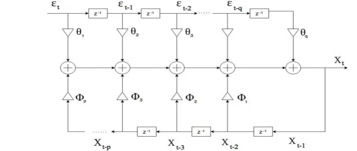
ARMA model plays an imperative role in the modeling of time series. It is a forecasting model [31]. ARMA represents a time series that changes uniformly around a time-invariant mean. The model offers a parsimonious description of a stationary stochastic process in the form of two polynomials, one for the autoregression and another for moving average. They model an unknown process with the least number of parameters. In order to make time-series stationary, the ARMA process removes trend and seasonal structures that negatively affect the regression model. Fig.1 represents the ARMA model.
Definition 1 (Autoregressive Moving Average). A stochastic process {Xt ;t ∈ Z} is an autoregressive moving average process of order (p, q), denoted with xt∼ARMA(p, q), if
q t q t
t p t p t
t X X
X
1 1...
1
1...
(1)Where tZ and φ1, ..., φp, θ1, ..., θqare set of AR(p) and MA(q) coefficients such that
0
,
0
qp
and {
t;
t
Z}.In ARMA model, the backward shift operator or lag operator (L) works on an element of a time series to move to prior element as
1
t
t X
LX (2)
and to move back to k element as k t t k
X X
L (3)
The autoregressive and moving-average polynomial are
ppL
L
L
1 1 (4)
qqL
L
L
1 1 (5)
Using backward shift operator in (3), the stochastic difference equation defining the ARMA process can be written as
t t L
X
L
( ) ( )(6)
IV. PROPOSED METHODOLOGY
Market basket database falls in the category of multivariate time series where each variable is influenced by varying time. Consequently, it can be modeled by multivariate ARMA models. Often, such databases include complex relations among individual series. In this paper multivariate ARMA model has been applied to find the dependency of the present dataset on past datasets in order to analyze customers buying behavior.
A. Multivariate Time Series
[image:3.595.93.442.578.726.2]Definition 4 (Multivariate Time Series): A multivariate time series (MTS) [32] comprises of individual time series, denoted by (𝑇𝑆1,2,𝑇𝑆3,…,𝑇𝑆k).
Fig. 1: Representation of ARMA Model
Hence, a set of k time series can be represented at t by the vector TSt=(TSt1,TSt2,…,TStk)
T
(7)
The k-dimensional multivariate ARMA(p,q) for the stationary time series can be expressed as
q t q t t t t p t p t t
t
Z
Z
Z
Z
1 1
2 2
...
1
1
2
2
...
(8)Where
kkr r
k r k
kr r
r
kr r
r r
...
.
...
.
.
...
...
2 1
2 22
21
1 12
11
is the rthARparameter matrix of order
k
k
for r = 1,2,….,p.is the rthMAparameter matrix of order k x kfor r = 1,2,….,q. B. Preprocessing of ARMA-ITARM
The key idea to use the ARMA model is to optimize window size to generate efficient and accurate temporal association rules in minimum time. In general, time-series data are collected and updated at a certain time interval (years, days, hours or minutes). However, it needs to be processed before the mining operation. Following steps are used in the pre-processing phase:
Stationarity testing and smoothing process
Determining size of p and q parameters by ACF and PACF graphs
ARMA model fitting is made by processed data and parameter values calculated from the previous steps Transformation of Time series data is converted into
transactional database by adding time dimension.
C ARMA-ITARM Algorithm
The algorithm ARMA-ITARM is used for incremental mining of TARs from time series database after preprocessing. It uses parameters p and q (obtained in preprocessing phase) to identify the number of correlated partitions (lag operator) and size of the window. Original database DBm,nis preprocessed before incremental mining to
find the parameters p and q. The ARMA-ITARM algorithm deals withthe maintenance of frequent itemsets and temporal association rules after updating original database in a time-variant transactional database.
Initially, database is partitioned based on preferred time granularity namely Pm,Pm+1,…,Pn. After preprocessing of
n m
DB ,
, number of partitions h and window size
w
is set by p and q respectively. Ifh
w
, i.e lag operator is not less than window size, incremental procedure is employed on newly arrived partition (n+1) after eliminating earlier r partitions (r
n
h
) partitions fromDB
m,n. However, ifw
h
,r
n
w
partitions are removed from the database and only recentw
partitions, i.e. DBmr,nare used as original database for incremental mining of Pn1.Algorithm ARMA-ITARM follows a probabilistic approach and keeps candidate 2-itemsets C2m,n generated in mining earlier partition. It is comprised of frequent 2-itemsets and probable frequent 2-itemsets.
Probable frequent itemsets are those itemsets that have a high probability to be frequent in the next partition; hence it is also forwarded to mining process of successive partition
,
represent the partitions to be removed and added respectively to the ongoing transaction database. . Fig. 2 shows working model of the algorithm.D
denotes the unaffected portion of the databaseFig.2: Working Model of ARMA-ITARM
.
The removed and incremental partitions are
m r 1m t
P
t(9)
kri r
k r k
kr r
r
kr r
r r
...
.
...
.
.
...
...
2 1
2 22
21
1 12
11
n m m P P
1
P
m (10)The old transactions
are removed from DBm,nand thenew transactions
are added. The updated database can be calculated by using the expression as, mn j
i
DB
DB, , . (11)
[image:5.595.312.538.59.709.2]Table I describes the meaning of the symbols used in proposed algorithm
.
Table-I: Symbols and their meaning
Symbols Meaning of Symbols
DBm,n Original database db Incremental database
UB Updated database
minsup Minimum support threshold probsup Probable support threshold h Number of unchanged partition
w Window size
n Number of last segment C2DB Candidate 2-itemsets in DB C2db Candidate 2-itemsets in db C2UB Candidate k-itemsets in UB CPF Probable frequent 2-itemsets in UB F2UB Frequent 2-itemsets in UB
X, Y Itemsets
XMCP(X) Itemset with exhibition period X.supp Support of X in segment p X.supDB Support of X in DB X.supdb Support of X in db X.supUB Support of X in UB |Pt | Size of any segment t TI Temporal candidate set SI, ST Subsets of TI L1 Frequent 1-itemsets TFI Temporal frequent itemsets
The unchanged transaction can be calculated as,
mn i j
DB DB
D , , (12)
Here,
denotes the incremental database db. Lastly, to generateL
k in the whole database, it performs the scanningon
DB
i,j only once to maintain frequent itemsets in the updated database.The incremental procedure can be further divided into the following sub-steps as:
Finding candidate 2-itemsets in D
Generating candidate 2-itemsets inD. Searching the database Donce to find all
frequent k-itemsets
L
k.In the first sub-step, candidate 2-itemsets in
mn
DB
D , is generated. The second sub-step
generates the new prospective
C
2i,jin DBi,j Dbyadding candidate itemsets in
D
and candidate itemsets in
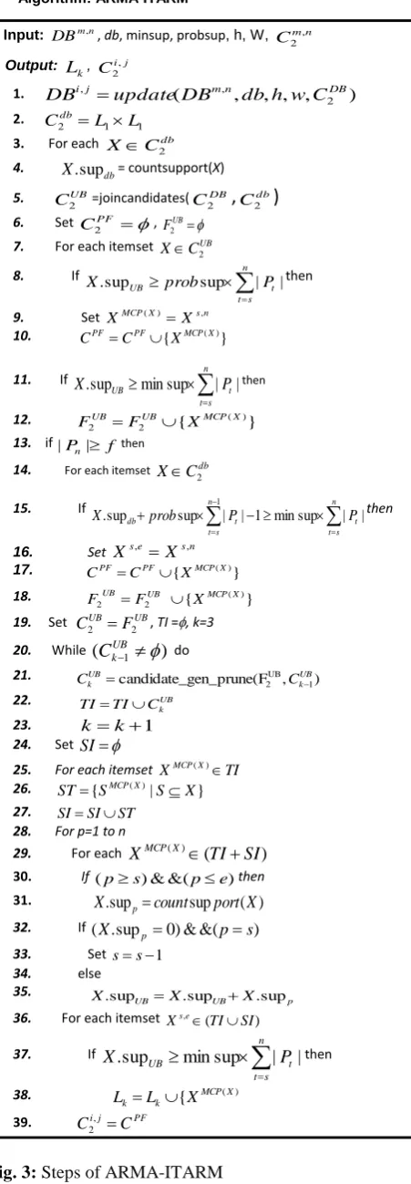
. Fig. 3 shows the steps of ARMA-ITARM.Algorithm: ARMA-ITARM
Input: DBm,n, db, minsup, probsup, h, W, mn
C , 2
Output:
k
L , i j
C, 2
1. DBi,j update(DBm,n,db,h,w,C2DB)
2. C2db L1L1
3. For each db
C
X 2
4.
db
X.sup = countsupport(X)
5. UB
C2 =joincandidates(
DB
C2
,
db
C2
)
6. Set PF
C2 ,
UB F2 7. For each itemset UB
C X 2
8. If
n s t t UB prob P
X.sup sup | |then
9. Set MCP X sn X
X ( ) ,
10. PF PF { MCP(X)} X C
C
11. If .sup minsup
| | n s t t UB P X then
12. { ( )}
2 2 X MCP UB UB X F
F
13. if|Pn| f then
14. For each itemset db
C X 2
15. If
sup 1| | 1 minsup | | sup . n s t n s t t t
db prob P P
X then
16. Set Xs,e Xs,n
17. PF PF { MCP(X)}
X C
C
18. { ( )}
2 2 X MCP UB UB X F
F
19. Set CUB FUB
2
2 , TI =, k=3 20. While ( UB1
)k
C do
21. candidate_gen_prune(F , )
1 UB 2 UB k UB k C
C
22. UB
k
C TI
TI
23. kk1 24. Set SI
25. For each itemset XMCP(X)TI
26. { ( )| }
X S S
ST MCPX
27. SISIST
28. For p=1 to n
29. For each XMCP(X)(TISI)
30. If (ps)&&(pe)then
31. X.sup countsupport(X)
p
32. If (X.supp0)&&(ps)
33. Set ss1 34. else
35.
p UB
UB X X
X.sup .sup .sup
36. For each itemset Xs,e(TISI) 37. If .sup minsup
| | n s t t UB P X then
38. ( ) { MCPX
k k L X
L
39. ij PF
C
C,
2
Fig. 3: Steps of ARMA-ITARM
Scan reduction technique is employed to generate
C
ki,j [image:5.595.58.278.183.457.2]1)size of the incremental partition is greater than f [32], where
2) Itemset is frequent in db
3) Sum of support count of itemset in db and minsup threshold in DB is more than
min
sup
|
,||
db
DB
i j
Lastly, to generate
L
k in the entire database, it performs one time scanning onDB
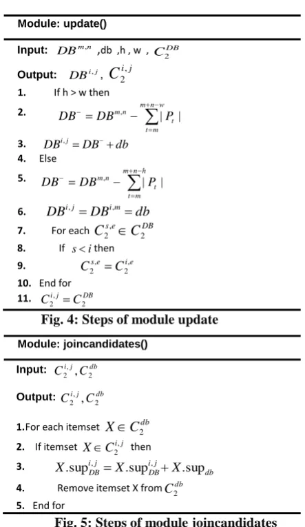
i,j to maintain frequent itemsets in the updated database. Fig. 4-6 shows the steps of modules update(), joincandidates and candidate_gen_prune() respectively.Module: update()
Input: DBm,n ,db ,h , w , DB
C2
Output: DBi,j,
C
i,j 21. If h > w then
2. ,
| | m nw
m t
t n
m
P DB
DB
3. DBi,jDBdb
4. Else
5. ,
| |
mn h
m t
t n
m
P DB
DB
6. DBi,j DBi,m db
7. For each Cs,e C2DB
2
8. If sithen
9. Cse Ci,e
2 ,
2
10. End for
11. ij DB
C
C 2
[image:6.595.53.275.226.609.2], 2
Fig. 4: Steps of module update
Module: joincandidates()
Input: ij db
C
C 2
, 2 ,
Output: ij db
C
C 2
, 2 ,
1.For each itemset XC2db
2. If itemset X Ci,j
2 then
3.
db j
i DB j
i
DB X X
X.sup, .sup, .sup
4. Remove itemset X fromCdb
2
5. End for
Fig. 5: Steps of module joincandidates
IV.EXPERIMENTALSTUDYANDRESULTS In order to evaluate the performance of ARMA-ITARM, several experiments has been performed on a system comprising following features: Intel(R) Core(TM) i3-3217U CPU with processing speed 1.80 GHz and 2.00 GB RAM inWindows 8.1 platform. The simulation program is coded in Java Netbeans IDE. Datasets are taken from frequent itemset mining repository. Following
sections describe about
datasets and presents performance comparison of ARMA-ITARM and SWF based on run time and Memory utilization by different algorithms.
Module: candidate_gen_prune()
Input: UB
k UB
C F2 , 1
Output: UB
k
C
1. UB k
C
2.For each pair UB k
C
XandY 1
3. If X[1,2,.,k -2] Y[1,2,..,k-2] then
4. If UB
F k Y k
X[ 1] [ 1] 2
5. C CUB (X Y) k
UB
[image:6.595.309.545.496.581.2]k 6. End for
Fig. 6: Steps of module candidate_gen_prune
A. Datasets
The datasets used for evaluation of the proposed algorithm ARMA-ITARM are primarily taken from frequent itemset mining database repository (FIMI, 2019) [33] and synthetic databases. Time attribute is incorporated in these datasets to be used as time series database. These datasets are partitioned based on time granularity imposed. We have partitioned database in order to test our algorithm and compare it with state-of-the-art algorithms ITARM and SWF. Table II describes the datasets used for performance evaluation of the proposed algorithm. For every update, the algorithm ARMA-ITARM, without the loss of generality, first set new original database as
i j mnDB
DB
D
, ,Table- II: Characteristics of datasets
Dataset DB size Db size items Trans_size
Accidents 1,20,000 2288 402 32
Retail 85,162 3000 16,470 13
T10D100kd10k 1,00,000 10,000 1000 10
T40D100kd10k 1,00,000 10,000 1,000 40
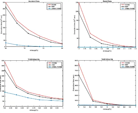
B. Runtime Performance Evaluation
Several experiments have been performed on different transaction datasets for all the three algorithms ITARM, SWF and ARMA-ITARM. Since the datasets have different characteristics, minimum support and probable minimum support are set for different datasets accordingly. Fig. 7 shows the outcome of the results of the experiments. Runtime difference of ITARM and SWF is consistent throughout for all the datasets. The reason for lesser execution time in SWF sup
min 1
| | sup) sup
(min
prob DB
Fig. 7: Runtime for various set of dataset
compared to ITARM is, SWF has fixed window size. It reduces the size of the original database by removing the least recent partitions. In ITARM, there is no such limitation. However, ARMA-ITARM also reduces the size of the original database and also it generates a lesser number of candidate itemsets, hence its execution time is very less compared to state-of-the-art algorithms
C. Memory Usage Analysis
Although all the three algorithms utilize scan reduction technique for k-itemsets generation, the memory requirement of ARMA-ITARM is low. . Fig.8 shows memory usage by the three algorithms.
Fig.8: Memory requirement in different datasets
[image:7.595.310.545.618.723.2]The algorithms ITARM and SWF consider all frequent itemsets of their prior database and incremental database (db), consequently generate a large number of candidate itemsets That further increases their memory requirement. On the other hand, ARMA-ITARM considers only those frequent itemsets from db that are high probability to be frequent throughout the database after updating. Hence, it generates a limited number of candidate itemsets. In ARMA-ITARM, the number of candidate itemsets is very close to actual frequent itemsets in the updated database. Hence, its memory requirement is very less compared to ITARM and SWF algorithms. Table III summarizes the results of different experiments.
Table-III: Summary of the experimental results
Algorithm Database size
Execution Time
Memory usage
Scalability
ITARM Large High in
dense datasets
Large Scalable
SWF Reduced Relatively
lower than ITARM
Relatively Smaller than ITARM
Scalable
ARMA-ITARM Relatively lower than SWF
Very low compared to both algorithms
Very small compared to both algorithms
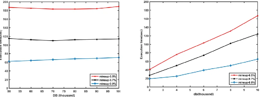
[image:7.595.60.271.620.768.2]Fig. 9: execution time in progressive database for minsup 0.5%, 0.7% and 0.9% D. Scalability Performance
To study the scalability performance of the algorithm, for a fixed value of minsup and probsup, experiments have been conducted by varying database size. Fig.9 shows the variation in runtime at different minsup. A progressive DB increasing with a fixed number of transactions shows a consistency in the runtime performance with increasing database size. While a db increasing with fixed number of transactions shows a consistent growth in execution time.
VI. CONCLUSION
Data mining is an important research domain that supports customers‟ buying behavior analysis. Various techniques were suggested to identify customers‟ preferred itemsets and buying patterns in static databases. However, these techniques are not suitable in a time-variant database. To deal with the time-variant database, this paper has suggested an incremental temporal association rule mining method. It identifies change in customers‟ behavior by discovering changed frequent itemsets. The ARMA model has been adopted to eliminate unrelated partitions and reduce the size of the working database. Based on this model, the proposed algorithm ARMA-ITARM defines the size of the sliding window. Due to the reduced database, its execution time and memory requirement is less. Experiments were conducted on available datasets and synthetic datasets and the performance of the proposed algorithm is compared with state-of-the-art algorithms. Results showed that ARMA-ITARM outperformed over ITARM and SWF algorithms. Hence, the proposed approach is efficient to mine updated temporal frequent patterns and consequently customers‟ changing behavior in a time series database.
REFERENCES
1. M. S. Chen, J. Han and P. S. Yu, “Data mining: an overview from a
database perspective,” IEEE Transactions Knowl. Data Eng, vol. 8,
no. 6, pp. 866-883, Dec. 1996.
2. D. T. Larose and C. D. Larose, “Discovering Knowledge in Data: An Introduction to Data Mining”, India: Wiley, 2014, pp. 1-14.
3. R. Agrawal and R. Srikant, “Fast Algorithms for Mining Association Rules,” in Proc. VLDB, 1994, pp. 87-499.
4. J. M. Ale and G. H. Rossi, “An approach to discovering temporal association rules,” in Proc. SAC, Como, Italy, 2000, pp. 294–300, DOI: 10.1145/335603.335770.
5. A. Vidhu and T. Shibili, “Network Intrusion Detection Using Temporal Association Rules,” Int. J. Sci. Eng. Res., vol. 5, no. 4, pp. 378-381, 2014.
6. V. Ng, S. Chan, D. Lau and C. M. Ying, “Incremental mining for temporal association rules for crime pattern discoveries,” in Proc ADC, Ballarat, Victoria, Australia, 2007, pp. 123-132.
7. G. Mao, “Mining temporal association rules in network traffic data,” Int. J. Future Comput. Commun., vol. 3, no. 1, pp. 55-59, Feb. 2014, DOI: 10.7763/IJFCC.2014.V3.267.
8. A. Raorane and R. V. Kulkarni, “Data mining techniques: A source
for consumer behavior analysis,” Int. J. Database Manage. Syst., vol.
3, no. 3, pp. 45-56, Aug. 2011, DOI: 10.5121/ijdms.2011.3304. 9. D.W. Cheung, J. Han, V.T. Ng and C. Y. Wong, “Maintenance of
discovered association rules in large databases: An incremental updating technique,” in Proc. Data Engineering, New Orleans, LA, USA, 1996, pp. 106-114.
10. C. W. Lin, T. P. Hong and W. H. Lu, “The Pre-FUFP algorithm for incremental mining,” Expert Syst. Appl., vol. 36, no. 5, pp. 9498-9505, Jul. 2009, DOI: 10.1016/j.eswa.2008.03.014.
11. A. F. Dafa-Alla, H. S. Shon, K. E. Saeed, M. Piao, U. I. Yun, K. J. Cheoi and K. H. Ryu, “IMTAR: incremental mining of general temporal association rules,” J. Inf. Process. Syst., vol. 6, no. 2, pp.163-176, 2010, DOI:10.3745/JIPS.2010.6.2.163.
12. J. Liu, Y. Gu and S. Kamijo, “Customer behavior classification
using surveillance camera for marketing,” Multimedia Tools Appl.,
vol. 76, no. 5, pp. 6595-6622, Mar. 2017.
13. M. K. Sharma, “The impact on consumer buying behaviour:
Cognitive dissonance,” Global J. Finance Manage., vol. 6, no. 9, pp.
833-840, 2014.
14. H. C. Chang, an H. P. Tsai, “Group RFM analysis as a novel
framework to discover better customer consumption behavior,” Expert Syst. Appl., vol. 38, no. 12, pp. 14499-14513, Dec. 2011, DOI: 10.1016/j.eswa.2011.05.034.
15. Z. Zhou, L. Shangguan, X. Zheng, L. Yang and Y. Liu, “Design and
implementation of an RFID-based customer shopping behavior
mining system,” IEEE/ACM transactions networking, vol. 25, no. 4,
pp. 2405-2418, Apr. 2017, DOI: 10.1109/TNET.2017.2689063.
16. C. Migniot and F. Ababsa, “3D human tracking from depth cue in a
buying behavior analysis context,” in Proc. CAIP, York, UK, 2013,
pp. 482-489.
17. E. P. Bafghi, “Clustering of Customers Based on Shopping Behavior
and Employing Genetic Algorithms,” Eng. Technol. Appl. Sci. Res.,
vol. 7, no. 1, pp. 1420-1424, Jul. 2016.
18. C. H. Lee, M. S. Chen and C. R. Lin, “Progressive partition miner:
an efficient algorithm for mining general temporal association rules,”
IEEE Transactions Knowl. Data Eng., vol. 15, no. 4, pp 1004-1017, Jul. 2003, DOI: 10.1109/TKDE.2003.1209015.
19. Z. Liang, T. Xinming, L. Lin and J. Wenliang, „Temporal Association Rule Mining based on T-Apriori Algorithm and its typical application,” in Proc. SYMP. Spatio-temporal Modeling, Spatial Reasoning, Analysis, Data Mining and DataFusion, 2005.
20. J. Ni, B. Cao, B. Yao, P. Yu, and L. Li, “ARTAR: Temporal
association rule mining
algorithm based on attribute
Wuhan, China, 2016, pp. 350-353.
21. E. Winarko and J. F. Roddick, “ARMADA–An algorithm for discovering richer relative temporal association rules from interval-based data,” Data Knowl. Eng., vol. 63, no. 1, pp. 76-90, Oct. 2007, DOI: 10.1016/j.datak.2006.10.009.
22. K. Verma, O. P. Vyas and R. Vyas, “Temporal approach to
association rule mining using t-tree and p-tree,” In Proc. IWMLDM
Pattern Recognition, Springer, Berlin, Heidelberg, 2005, pp. 651-659.
23. M. M. Fouad and M. G. Mostafa, “IndxTAR: An Efficient Algorithm for Indexed Mining of Incremental Temporal Association Rule,” Int.J. Comput. Inf. Syst. Ind. Manage. Appl., vol. 9, pp. 103-113, 2017.
24. S. Shalini and K. Lal, “Mining Changes in Temporal Patterns in Latest Time Window for Knowledge Discovery,” J. Inf. Knowl. Manage., to be published.
25. A. S. Al-Hegami, “A Framework for Incremental Mining of
Interesting Temporal Association Rules,” Int. J. Comput. Appl., vol.
131, no. 8, pp. 28-33, Dec. 2015, DOI: 10.5120/ijca2015907433.
26. J. Huang and W. Wei, “Efficient algorithm for mining temporal
association rule,” Int. J. Comput. Sci. Network Secur., vol. 7, no. 4, pp. 268-271, Apr. 2007.
27. T. F. Gharib, N. Hamed, M. Taha and A. Abraham, “An efficient
algorithm for incremental mining of temporal association rules,” Data Knowl. Eng., vol. 69, pp. 800-815, Aug. 2010, DOI:10.1016/j.datak.2010.03.002.
28. M. Naqvi, K. Hussain, S. Asghar and S. Fong, “Mining temporal association rules with incremental standing for segment progressive filter,” in Proc. ICNDT, Springer, Berlin, Heidelberg, 2011, pp. 373-382, 10.1007/978-3-642-22185-9_32.
29. T. C. Fu, "A review on time series data mining," Eng. Appl. Artif. Intell., vol. 24, no. 1, pp. 164-181, Feb. 2011, DOI: 10.1016/j.engappai.2010.09.007.
30. M. C. Chen, A. L. Chiu, H. H. Chang, “Mining changes in customer behavior in retail marketing,” Expert Syst. Appl., vol. 28, no. 4, pp. 773-781, May 2005, DOI: 10.1016/j.eswa.2004.12.033.
31. Z. Zhang and J. C. Moore, “Autoregressive Moving Average Models,” Math. Phys. Fundam. Clim. Change, 2015, Pages 239-290, DOI: 10.1016/B978-0-12-800066-3.00008-5.
32. Y. Zhao and T. T. Zhang, “Discovery of Temporal Association Rules in Multivariate Time Series,” in Proc. ICMMSTA, 2017, DOI: 10.12783/dtcse/mmsta2017/19653.
33. T. P. Hong, C. Y. Wang and Y. H. Tao, “A new incremental data mining algorithm using pre-large itemsets,” Intell. Data Anal., vol. 5, no. 2, pp. 111-129, Apr. 2001, DOI: 10.3233/ida-2001-5203. 34. Frequent Itemset Mining Dataset Repository: Available online at:
http://fimi.ua.ac.be/data/ (Accessed on 6th july 2019)
AUTHORSPROFILE
Sheel Shalini is an Assistant Professor in Computer Science and Engineering Department at Birla Institute of Technology Mesra, Patna Campus, India. She is pursuing her Ph. D from Birla Institute of Technology, Mesra in Data Mining. She has master‟s degrees in Computer Science (M.Tech) from Allahabad Agriculture Deemed University, Allahabad, India, and Computer Application (M.C.A.) from Lalit Narayan Mishra Institute of Economic Development and Social Changes, Patna, India. She also holds M.Sc.in Physics from Patna University, Patna, India. She has 25 years of teaching experience in various fields of Computer Science. Her research interests include data mining, database management and algorithms design
Kanhaiya Lal is an Assistant Professor in Computer Science and Engineering Department at Birla Institute of Technology Mesra, Patna Campus, India. He completed his B. Engg (CSE), M. Tech(CSE) and Ph. D from Birla Institute of Technology, Mesra, India. He has 25 years of teaching experience in Computer Science. His areas of interest include Artificial Intelligence and Data Mining. He has published number of articles and research papers. He is an author of the book titled Semantic Web Based Data Cloud and co-author of Energy Deviation and Control. He is a member of ACM, IAENG, ISAI, IEI and CSI India.