doi:10.1017/S0022112007006921 Printed in the United Kingdom
Rough-wall boundary layers: mean flow
universality
I A N P. C A S T R O
School of Engineering Sciences, University of Southampton, Highfield, Southampton SO17 1BJ, UK [email protected]
(Received14 December 2006 and in revised form 2 May 2007)
Mean flow profiles, skin friction, and integral parameters for boundary layers develop-ing naturally over a wide variety of fully aerodynamically rough surfaces are presented and discussed. The momentum thickness Reynolds number Reθ extends to values in excess of 47 000 and, unlike previous work, a very wide range of the ratio of roughness element height to boundary-layer depth is covered (0.03< h/δ <0.5). Comparisons are made with some classical formulations based on the assumption of a universal two-parameter form for the mean velocity profile, and also with other recent measurements. It is shown that appropriately re-written versions of the former can be used to collapse all the data, irrespective of the nature of the roughness, unless the surface is very rough, meaning that the typical roughness element height exceeds some 50 % of the boundary-layer momentum thickness, corresponding to about h/δ>0.2.
1. Introduction and background
when h/δ is sufficiently large for changes to occur in the latter, the former might well retain a more classical behaviour. Although he did not state it explicitly, it can be deduced from Hama’s paper that the maximum h/δ reached was somewhere in the range 0.3–0.5. With the hindsight of half-a-century, it is evident that this now classical work has some major shortcomings (see below), not least in that only a single roughness geometry was tested, but the resulting correlations have been the basis of a number of works since. It is the intention here to show that despite the deficiencies in the data, Hama’s overall conclusion is valid for a wide variety of roughness geometries and that appropriate formulations of some of the later classical mean flow correlations are very resilient and thus provide useful results for surprisingly largeh/δ. A careful reading of some of the more recent literature suggests that some of the lessons of the 1950s and 1960s have been forgotten and we therefore begin with a brief review of mean flow formulations and some of the more modern extant data.
The effect of surface roughness on the boundary-layer mean velocity profile is classically expressed using a roughness function U+, which modifies the usual smooth-wall formulation, as expressed below for the fully rough case,
u+ ≡ U uτ
= 1
κln
(y−d)uτ
ν
+A−U+(h+), (1.1)
in the usual notation, but with inclusion of a zero plane displacement,d. For a smooth wall this would be zero, unless during the experiments the measured wall-distance was in error by some small amount. (The expected conformity with the smooth-wall version of (1.1) is sometimes used to deduce this error.) For a rough wall, with y
measured from the bottom of the roughness elements, d can be interpreted as the effective height of momentum extraction and is always less thanh. Jackson (1981) has shown that this height – essentially the height at which the mean surface drag appears to act – is implicit in the derivation of the log law. In general,U+ is a function of h+ and the geometrical parameters defining the element shapes and arrangement – what we might call the roughness texture. In (1.1), we limit this dependence to element height, h. The alternative way of expressing the rough-wall profile in cases of fully rough surfaces (when viscous effects at the the surface are negligible), favoured by the meteorological community for whom fully rough conditions almost always pertain, is to write
u+≡ U uτ
= 1
κ ln
y−d y0
. (1.2)
y0 is the roughness length, which embodies the effect of the roughness function in (1.1) and is determined byhand the roughness texture alone.U+ andy
0 are simply alternative, but entirely equivalent, measures of the roughness and are related via
U+=A+ 1
κ ln(Re
∗)≡A+ 1 κln(h
+) + 1 κ ln
y0
h
, (1.3)
of the roughness geometry (as also, incidentally, isd/ h). Attention is concentrated in this paper on fully rough cases, where viscous scales such asν/uτ are not relevant, so we use (1.2) and thus y0 as the appropriate scale defining the roughness (rather than h+). We are not concerned here with the nature of the relationship between geometry and the resulting y0 (but see the Jim´enez 2004 and Raupachet al. 1991 reviews for some examples of such work).
The profile expressions above can be modified to include the outer flow, usually expressed by a wake function in the form of an additional term, (Π/κ)w(y/δ), added to the right-hand side of (1.1) (or (1.2)).Π is the Coles (1956) wake parameter withw
assumed to be a universal function of y/δ– at least for zero-pressure-gradient flows. The complete (two-parameter) profile can then be written in defect form as
Ue−U
uτ
=−1
κln y δ +Π κ
2−w
y δ
, (1.4)
independently of wall type or the specific functionwchosen as the wake profile (and note that w(1) = 2 and0∞wd(y/δ) = 1). Note also that in (1.4) and the expressions that follow, y and δ are to be understood as (y−d) and (δ−d). Throughout this paper we employ the common definition of δ as the point where the mean velocity is 99 % of its free-stream value. In his seminal treatise on boundary layers, Rotta (1962), following Clauser (1954), defined a parameterI (Clauser’sG) by
I=
∞
0
Ue−U
uτ 2 d y , (1.5)
where=δ∗Ue/uτandδ∗is the usual displacement thickness. Employing the standard definitions for δ∗ and the momentum thickness,θ, leads to
I = H −1
H Ue
uτ ≡
H−1
H
2
Cf
, (1.6)
whereH is the usual shape parameter,δ∗/θ. I is a function only of w,Π and κ and for most wake profile shapes that have been used, can be expressed as I= (a+bΠ+
cΠ2)/κ/(e+Π), where a, b, c and e are numerical constants whose values depend only on the specific profile shape. (For example, for the quartic polynomial wake profile suggested by Lewcowicz (1982)I= (2.009+3.018Π+1.486Π2)/[κ(0.983+Π)], compared withI= (2 + 3.2Π+ 1.522Π2)/[κ(1 +Π)], which arises from Coles’ profile). It also follows directly that
δ ≡ δ∗ δ Ue uτ
≡ δ∗ δ
2
Cf
= 1 +Π
κ . (1.7)
Note thatH= (1−I uτ/Ue)−1and that (1.2)–(1.7) are independent of the nature of the surface and assume only that the two-parameter profile is an adequate representation of the mean flow (and, for the smooth-wall case, that the viscous sublayer can be ignored in the integrations for θ and δ). Clauser (1954) and Rotta (1962) derived the resulting relation between surface friction, Cf≡2(uτ/Ue)2, and θ. Using (1.2) rather than (1.1) to describe the log-law in the fully rough case, this relation can be re-written more conveniently as
2
Cf =−1
κ ln 1 H Cf 2 + 1 κ ln θ y0
whereK= 2Π /κ−(1/κ) ln((1 +Π)/κ), and this can be rearranged to give
θ y0
= s−I
s2 e
κ(s−K), (1.9)
wheres=2/Cf. The use of the roughness length,y0, removes the need to consider A and U+ (in (1.1)) separately and also, as indicated above, assumes that it is determined solely by the specific roughness geometry. Notice in particular that all the above implies, quite generally, that H=f1(Cf, Π, κ) and that, for a fully rough surface, H=f2(θ/y0, Π, κ), Cf=f3(θ/y0, Π, κ). This means that given f1, both Cf andH can be calculated as a function ofθ/y0, provided that κ is known and thatΠ is not dependent on the roughness type.
There is some evidence that even if a universal wake function is accepted for all kinds of boundary layers, the value ofΠ is significantly higher for rough-wall than for smooth-wall flows. Tani (1987), for example, re-analysed a number of previously reported data sets and found values between 0.4 and 0.75 for various types of roughness. It is difficult to obtain accurate values of Π – partly because it arises as the difference between two relatively large quantities. It is also very sensitive to the precise values chosen for the log-law constants. Recognizing the uncertainty about whetherΠ truly is constant, Krogstad et al. (1992) used a fitting procedure for the entire velocity profile (in defect form) which did not constrainΠ but optimized values of uτ, d and Π to provide the best fit (to an assumed form of the wake profile w), assuming thatκ= 0.41. For their mesh roughness they found thatΠ= 0.7. This also led to good agreement between the optimized uτ and the uτ deduced from direct measurements of the turbulence shear stress. Following Perry, Lim & Henbest (1987) who were perhaps the first to demonstrate the inadequacies in standard hot-wire anemometry near rough walls, they used high-accuracy hot-wire anemometry – i.e. 120◦ cross-wire probes. Perry et al.also fitted the entire profile using Hama’s (1954) inner and outer region relations and thus implicitly assumed a value for Π (about 0.51). Likewise, Bergstrom, Akinlade & Tachie (2005) made measurements over sand grain, perforated plate and wire mesh surfaces and, using a procedure similar to Krogstad’s, found Π values between 0.5 and 0.65, with the highest values coming from the fully rough (rather than transitional) cases. In terms of the relationship between H and Cf given by (1.6) their data conformed well to I= 7.0; but this immediately implies a fixed value forΠ of about 0.7 (given their wake profile shape) and a value for what they called the modified skin friction parameter,Cf(δ/δ∗), of 0.341. In proposing the latter as a ‘new skin friction correlation’ they appeared not to recognize that it follows directly from (1.7). Actually, they suggested a value of 0.36±0.025 for this parameter which, strictly, is not consistent with theirI≡G= 7.0. Note that Bergstrom et al.defined δ as the point at which the velocity was 99 % of the free-stream value which, as noted earlier, is the present definition.
graphical differentiation of the measuredθ. In addition to the uncertainties associated with that process, even given good two-dimensionality of the flow, the mean velocity profiles were obtained using Pitot tubes without any correction for turbulence effects. This is likely to have led to significant errors, given the relatively high values of turbulence intensity near rough surfaces, particularly for cases of large h/δ. Their data thus suggest correlations noticeably different from those arising from more modern experiments, as shown later.
In the present paper, the new data sets reported were all obtained in conjunction with hot-wire and/or laser-Doppler anemometry shear stress measurements, so that
Cf is known independently. The experiments cover a range of roughness types, including arrays of sharp-edged cuboid obstacles, and also include data at relatively short distances from the leading edge of the roughness, so that h/δ reached values much larger than in any previous experiments. The intention is to demonstrate that the classical formulations based on a two-parameter profile family (i.e. (1.4)–(1.8) but with a more recent wake profile shape than Coles’ original) provide an adequate fit to the data over a wide range of θ/y0, with a fixed value of Π = 0.7, and independent of the nature of the roughness geometry. The experiments are summarized in the following section, §3 presents the results and final discussion and conclusions are given in§4.
2. Experimental details
18
27 18
27 Flow
Thickness Width (a)(i)
(b)
(d)
[image:6.493.96.406.51.360.2](c) (ii)
Figure 1.Rough surfaces used. (a) Mesh roughness. Flow is from bottom to top (for (i)).
Thickness, axial and spanwise pitch are 3 9.7 and 28.6 mm. (b) Staggered cube arrays of 25 % area coverage (5 or 10 mm cubes). (c) FMF block roughness (25 % area coverage). Dimensions in mm (height 18). Flow from top to bottom. (d) FMF ‘sanspray’ gravel chip surfaces – average chip size 10 mm or 3 mm.
Chevray 1975). All the more recent HWA data were obtained using ±60◦ wires, which minimize these errors (see Perryet al. 1987). Data obtained with these probes, also corrected for high-turbulence effects because such corrections were not always negligible, were found to be quite close to those obtained using LDA, which provides some confidence in the accuracy of both. The probes were in all cases driven using standard CTA bridges whose outputs were filtered, amplified and digitized under the control of computers, allowing on-line calibration and measurement. Laser-Doppler anemometry data were obtained using a two-component Dantec fibre-optic probe mounted outside the tunnel. A 5 W argon-ion laser (typically operated at 1 W) was used, with the photomultiplier outputs collected and manipulated using burst spectrum analysers operating in coincidence mode. Data rates were up to 2 kHz, at least 2 min of sampling time was used at each traverse point, and transit-time data were used to provide corrections for bias errors arising from non-uniform sampling. The measurement volume was typically 2.4 mm in length (in the spanwise direction) and about 0.15 mm in diameter.
gradient within the working sections, arising from the boundary-layer growth on all four walls. However, this was always much smaller than that normally expected to have a measurable effect on boundary-layer flow.
3. Results
3.1. Skin friction and shape factor correlations
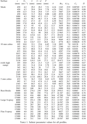
All the salient data used in the figures are given in table 1. We start by presenting skin friction and momentum thickness data. Here, Cf is defined in the usual way as the surface stress normalized by ρUe2/2, so that (uτ/Ue)2=Cf/2 as in the previous section, where uτ is by definition the wall friction velocity. This was determined by assuming that u2
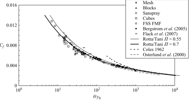
τ=−uv, where the latter is the turbulence Reynolds shear stress measured in the near-wall region of the flow and extrapolated to y=d. Note that throughout this work, x andy are the axial and wall-normal directions, respectively, with the origin at the start of the roughness. There is no point in showing the many individual velocity profiles obtained during the course of all the experiments. These each have exactly the expected and well-known behaviour. We concentrate on the resulting parameters. Figure 2 shows the variation ofCf withθ/y0, which corresponds toReθ for a smooth wall.θ was in every case calculated by appropriate integrations of the velocity profiles, with the very-near-surface region (between y−d = y0 and the nearest measurement point) modelled using extensions to the log-law fitted to the data just above that region. The latter fits (to (1.2)) were forced to have a slope consistent with the measured −uv and with a zero-plane displacement,d, adjusted to yield the best fit. Throughout the work, we tookκ= 0.41. For the reasons outlined in
§2 and because we had an independent measure of wall friction, we did not attempt to fit the entire velocity profile (with either an assumed or free value of Π) in order to determineCf. The roughness lengths, y0, followed directly from our fits forced to give log-law slopes consistent with the measuredCf. The fits naturally led to specific values of Π, which we discuss in due course. It is worth pointing out that although, within the roughness sublayer where the flow is spatially inhomogeneous, individual profiles are not necessarily logarithmic, it has been shown that spatially averaged mean velocities (at each height) do conform to extensions of the log-law region in the inertial layer above (Cheng & Castro 2002). So it is believed that this simple extrapolation of the velocity profile through the sublayer region is the best approach for determination ofθ (and δ∗). Nonetheless, there are inevitable uncertainties in the whole process, particularly at the largest h/δ, arising largely from the uncertainties inherent in measuring the turbulence shear stress,−uv, and using extrapolated values of the latter to give u2τ. Given the careful use of laser-Doppler anemometry and the appropriate corrections to HWA data, it is likely thatuτ errors are below ±7 %.
The data in figure 2 clearly collapse fairly satisfactorily for very different types of surface onto the classical result arising from a universal two-parameter profile, i.e. (1.9). Note that the latter is, in principle, dependent on the precise shape of the wake profile, through I. However, choosing, for example, either Coles’ (1962) original wake function as Rotta (1962) did, or Lewkowicz’s (1982) polynomial as Tani (1987) did, yields (for the same value of Π) curves which are indistinguishable above the thickness of the bold line in the figure. On the other hand, the result depends noticeably on the particular value of Π used; the bold solid line in figure 2 is the result with Π= 0.7 and it is noticeably lower than the result obtained using
Surface x Ue δ δ−d δ∗
(mm) (m s−1) (mm) (mm) (mm) θ Re
θ θ/y0 Cf Π
Mesh 450 4.2 29.2 28.2 7.51 4.14 1165 25.9 0.00769 0.75
450 8.3 29.4 28.6 7.78 4.26 2361 25.1 0.00720 0.80 450 12.5 31.6 29.4 7.37 4.13 3447 22.9 0.00819 0.79 450 16.8 31.5 28.8 8.00 4.40 4928 21.0 0.00845 0.55 1000 4.3 50.0 47.5 12.3 7.07 2032 32.3 0.00770 0.70 1000 8.8 48.7 46.3 11.4 6.46 3794 28.4 0.00700 0.83 1000 13.2 47.5 45 11.9 6.59 5812 27.7 0.00660 0.91 1000 17.0 48.4 45.4 12.1 6.52 7402 28.4 0.00684 0.98
2400 4.3 95 92 22.2 13.3 3839 44.3 0.00673 0.68
2400 8.7 89.3 81.8 20.3 12.1 7049 40.3 0.00650 0.78 2400 13.0 91.0 88.4 21.2 12.3 10 693 29.3 0.00732 0.71 2400 17.0 92.1 90 20.8 12.3 13 965 37.3 0.00673 0.67 3930 18.1 123.6 121 28.7 17.1 20 634 31.1 0.00641 0.89 3930 13.4 118 116 28.1 16.9 15 097 42.3 0.00620 0.79 3930 8.9 117 115 27.8 16.6 9849 41.5 0.00627 0.82 3930 4.4 114.7 113 26.8 16.2 4778 46.3 0.00620 0.78 10 mm cubes 105 10.0 32.1 22.6 6.42 3.14 2093 7.0 0.0128 0.71 185 10.2 35.2 25.2 7.37 3.57 2380 8.5 0.0119 0.69 345 10.3 40.4 31.4 9.61 4.86 3240 10.8 0.0101 0.78 655 10.6 50.6 41.6 11.8 6.31 4207 15.4 0.0090 0.73 1015 10.5 62.6 53.1 15.2 7.94 5293 14.4 0.00879 0.78 1245 10.5 61.2 60.7 16.8 9.14 6093 16.6 0.00840 0.74 2180 10.8 96.0 86 22.7 12.52 8347 26.1 0.00730 0.77 3130 10.9 119.5 110 27.5 15.7 10 473 33.4 0.00680 0.73 (with high 105 10.0 29.3 21.3 5.23 2.77 1847 13.9 0.00960 0.67
ramp) 185 10.1 31.4 22.4 5.78 3.14 2093 15.7 0.00960 0.64
345 10.2 36.2 26 7.17 3.9 2600 16.3 0.00980 0.61
[image:8.493.67.441.71.603.2]655 10.3 45.8 35.8 10.6 5.62 3747 14.8 0.00941 0.68 1245 10.5 65.1 55.1 16.2 8.5 5667 14.7 0.00919 0.71 2180 10.8 90.1 81.8 22.9 12.4 8233 18.5 0.00794 0.81 3130 10.9 113.6 104.1 26.4 15.3 10 200 31.9 0.00701 0.72 5 mm cubes 432 9.6 36.5 33.0 8.63 4.53 3020 15.1 0.00840 0.81 995 9.7 51.8 47.8 11.5 6.68 4453 26.7 0.00759 0.76 1543 9.9 64.5 62.1 15.1 9.05 6033 34.8 0.00700 0.76 2333 10.0 88.0 84.0 19.2 11.4 7627 45.8 0.00620 0.78 2985 10.2 100 96.1 21.8 13.2 8800 50.8 0.00580 0.81 Rect.blocks 6000 8.0 274.1 250 54.4 32.4 29 013 43.2 0.0065 0.73 10 000 8.0 368 350 77.6 47.7 41 387 68.1 0.00560 0.78 12 000 8.0 416 400 88.5 54.6 47 200 78.0 0.00530 0.84 15 000 8.0 449 430 89.6 58.0 47 787 116 0.0051 0.66 Large S-spray 6000 7.9 191.1 190 38.8 25.1 13 387 105 0.00529 0.61 8000 7.9 236 233 47.5 31.1 16 587 156 0.00461 0.73 10 000 7.9 287 285 57.4 37.7 20 107 151 0.00461 0.75 12 000 7.9 350 320 62.7 42.7 22 773 251 0.00410 0.73 15 000 7.9 385 385 72.7 50.2 26 773 279 0.00405 0.69 Fine S-spray 6000 4.0 181 180 34.8 22.6 6027 127 0.00508 0.62 10 000 4.1 242 240 49.0 31.8 8480 212 0.00460 0.58 12 000 4.1 290.5 290 55.1 36.6 9760 183 0.00462 0.64 15 000 4.1 311 310 57.0 39.7 10 587 305 0.00435 0.54
Table 1.Salient parameter values for all profiles.
solid curves in figure 2 are close to Coles’ smooth-wall line, which is here plotted on the basis that for a smooth wall, from (1.3) with U+= 0, y0= (ν/uτ) e−κA so that θ/y0= 7.768Reθ
0 0.004 0.008 0.012 0.016
100 101 102 103 104
θ/y0 Cf
Mesh Blocks Sanspray Cubes FSS FMF
Bergstrom et al. (2005) Flack et al. (2007) Rotta/Tani Π = 0.55 Rotta/Tani Π = 0.7 Coles 1962
[image:9.493.79.403.61.232.2]Osterlund et al. (2000)
Figure 2.Skin friction as a function of momentum thickness.
expected, since Coles’ calculated value for Π asymptotes to 0.55 at sufficiently large
Reθ (although he later adjusted it to 0.62, Coles 1987).θ/y0= 700 corresponds, for the smooth-wall case, to Reθ of about 2000 and for Reynolds numbers lower than this it is well known that Π falls monotonically, so the smooth-wall correlation naturally rises above the rough-wall data in that region, as seen in the figure. It is emphasized that the present rough-wall data span a wide range of Reθ and, because of the very different types of roughness employed, the variation in Reθ is not monotonic with
θ/y0; so in figure 2 the data point corresponding to Reθ= 47 800 (the largest), for example, lies nearθ/y0= 100.
The figure includes the data of Bergstrom et al. (2005) and of Flack, Schultz & Connelly (2007), which do not extend beyond Reθ= 13 000 in either case. It is clear that these are reasonably consistent with all the other data. (Note that for the latter set, the data have been re-analysed with the same methods as used for the present data, i.e.Cf was obtained from the LDAuvdata, log-law extrapolations down toy−d=y0 were used to obtainδ∗andθ, and theδ99thickness was used.) It should be emphasized that some degree of scatter is inevitable because the accurate determination of y0 is difficult. Small changes in the log-law slope (i.e. small changes in Cf) lead to large changes in y0. It is evident that the scatter increases as θ/y0 falls; there are various possible reasons for this. First, at this end of the θ/y0 range, the roughness height is not very small compared to the boundary-layer height. For example, the lowest two points for the cube roughness, withθ/y0= 7−9, have h/(δ−d)>0.4. With the exception of Hama’s (1954) data, which suffer from the difficulties mentioned above, these are way beyond values previously studied and one would perhaps not expect close conformity to a universal velocity profile. Secondly, at such large values of
0.001 0.010 0.100
1.2 1.4 1.6 1.8 2.0 2.2
H Cf
Blocks
Cubes Mesh
Bergstrom et al. (2005) Flack et al. (2007) Coles (1962) Hama (1954)
[image:10.493.102.408.58.240.2]From (1.6) with I = G = 7.03 Sanspray
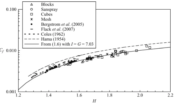
Figure 3. Shape factorH as a function ofCf, as predicted by (1.6), withΠ= 0.7.
only fall to amplitudes similar to those present in smooth-wall boundary layers once
h/(δ−d)<0.05. There is no reason to doubt that similar effects will occur for other roughness types. All these features make the deduction ofCf from turbulence shear stress data (or in any other way) rather uncertain. Indeed, for the mesh surface, for example, profiles obtained atx= 200 mm had a peak some way from the wall, before falling as the wall was approached. This was no doubt a result of the inevitably strong disturbance at the leading edge. Choosing this peak as a surrogate foru2
τ led to Cf data (havingθ/y0<10) which was scattered by up to±20 % about theΠ= 0.7 line shown in figure 2, so these data are not included.
The leading-edge disturbances could, in one sense, be considered as arising from a smooth-to-rough change of surface condition. There have been many experiments exploring the effect of roughness change on boundary-layer development (Antonia & Luxton 1971 was one of the earliest), but these have always been for cases when the upstream boundary-layer thickness (δ) is large compared with the roughness elements of the downstream surface. The results, usually couched in terms of how large a fetch is required before fully developed conditions are reached (typically around 20δ), are thus not very relevant to the present leading-edge regions, where the upstream boundary layer is very thin indeed – often smaller than the size of the roughness elements.
The relationship between Cf and H suggested by (1.6) is shown in figure 3 and overall the data are consistent with the value ofI (7.03), deduced using Π= 0.7. In this case, the result is a little more sensitive to the precise wake profile shape chosen, and the curve shown assumes the Lewcowicz (1982) quartic profile (as also used by Tani 1987). The Coles’ wake function (as used by Rotta) givesI= 7.15 withΠ= 0.7, leading to a curve noticeably higher than that shown in the figure, thus having a less satisfactory fit to the data. The smoothed line through Hama’s (1954) original data is included in the figure and it is evident that this is not such a good fit to the more recent data, as expected.
0 0.2 0.4 0.6
100 101 102 103 104
θ/y0 Cf1/2δ
——–
δ* Blocks
Sanspray Cubes Mesh
Bergstrom et al. (2005) Flack et al. (2007)
[image:11.493.74.408.54.220.2]Tani (1987) Coles (1962)
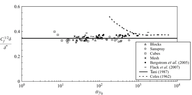
Figure 4. Modified skin friction, (1.7), compared with data.
a way that leavesΠ as a free parameter to be determined by the fit did not, for any given roughness type, produce identifiable trends in Π with, for example, increasing
θ/y0, nor any trends between roughness types. Given the imprecise nature of such fits, as discussed earlier, we do not believe such a process has particular merit and in view of the general degree of fit between the data and the classical correlations, illustrated by figures 2–4, it would seem that the latter provide adequate descriptions of the mean flow even for ‘very’ rough surfaces, which might be defined as those for whichh/δ > O(0.1). Notice, incidentally, the rise inCf/2(δ/δ∗) for the smooth-wall (Coles) correlation belowθ/y0≈1000, in line with the falling value ofΠ at these low Reynolds numbers, as noted earlier.
A final remark about figures 2–4 is worth making. The 10 mm cube surface data were obtained in two cases – with and without an upstream ramp. When present, the ramp was about 300 mm in length and its surface began at y= 0 and finished at the top of the cubes (y= 10 mm). Without the ramp, there was a much more severe distortion of the very thin oncoming boundary layer, no doubt with strong separated shear layers at the first row, leading to locally larger wall stresses – and no doubt greater spatial inhomogeneity. With the ramp, these initial distortions are minimized, but the degree of scatter at small fetches is not significantly lower.
3.2. Correlations with fetch
It is possible to use the momentum integral equation (MIE), dθ /dx=Cf/2, along with (1.6) and (1.9) to deduce howCf and thusθ andδ∗ will vary with fetch (x). This was done by Clauser (1954) and Rotta (1962). In a zero pressure gradient, using the present notation, the MIE yields
x=
2dθ Cf
=
s2dθ=s2θ−2
sθds. (3.1)
0.002 0.006 0.010 0.014
102 103 104 105 106
(x – x0)/y0 Cf
Blocks Sanspray Cubes
[image:12.493.104.408.57.208.2]Bergstrom et al. (2005) Schlichting (1968) From MIE with I = 7.03
Figure 5. Skin friction as a function of fetch.
δ* —y 0
Blocks - new an. Sanspray Cubes Mesh, x = 3930
Bergstrom et al. (2005) RLP (1976) From MIE
(a) 104
103
102
101
100
102 103 104 105 106 (x – x0)/y0
θ —y
0
Blocks Sanspray Cubes Mesh
Bergstrom et al. (2005)
From MIE
(b) 104
103
102
101
100
102 103 104 105 106 (x – x0)/y0
Figure 6. Momentum and displacement thicknesses.
specified. It seems most sensible to uses=I atx=x0 so that (3.1) can be written
x−x0=s2θ−2
s
I
θ(s)sds (3.2)
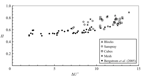
[image:12.493.78.431.241.516.2]0 0.2 0.4 0.6 0.8 1.0
10 15
∆U+ Π
Blocks Sanspray Cubes Mesh
Bergstrom et al. (2005)
[image:13.493.93.386.53.211.2]5
Figure 7. Variation ofΠ with roughness.
data compared with the corresponding correlations calculated from (1.9) and (1.6), respectively. Again, there is a good fit over all the range except at the lowest fetches. The data from Bergstomet al.(2005) have been included and these diverge noticeably at the upper end of the range, where the data are from the smallest roughness cases which, in fact, haveRe∗ <1 and are only transitionally rough. Nonetheless, theδ∗vs. (x−x0) correlation is in fact very insensitive to the precise form of the profile shape (and thus toΠ) and the curves shown are virtually indistinguishable from the smooth-wall equivalents. One expects transitional roughness data to collapse along with fully rough and smooth data, so the noticeably high values in Bergstrom’s data must be explained another way; they are probably (at least partly) a result of uncertainties in the virtual origin, which was not measured but for the present purposes was taken as being at a distance upstream of the leading edge similar to that found typically in the present data. Figure 6(b) also includes Ranga Raju, Loeser & Plate’s (1976) correlation, similarly covering smooth to fully rough situations. Based on Schlichting’s (1968) correlations, which assumed a one-seventh power-law profile, they proposed a
δ∗ formulation given by
δ∗ y0
= 0.05
x−x0
y0
7/9
. (3.3)
They were perhaps the first to suggest this kind of correlation and (3.3) is seen to be very close to the more precise result for (x−x0)/y0>2×104, but deviates noticeably at smaller fetches. To preserve clarity, their data are not included in the figure; those from the roughest of their surfaces are higher than their correlation, but fit the present more accurate one quite well.
serious disturbances to the boundary layer. This provides yet another reason for the scatter inΠ at small fetches; at these locations, one might on that basis not expect
Π to have ‘recovered’ from the leading-edge flow. It is concluded that although there is some evidence that Π rises with roughness, the calculations made on the basis that it remains constant (at around 0.7) provide very useful correlations which fit the experimental data to within the likely accuracy of the latter. For a sufficiently large fetch, of course,θ/y0 must eventually become so large that after a transitional region the flow would revert to a genuinely smooth-wall boundary layer, with the roughness elements well submerged within the viscous region; Π would then have the smooth-wall value (around 0.55).
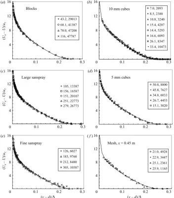
3.3. Velocity defect profiles
Finally, it is helpful to assess the universality of the velocity profiles when plotted in deficit form. Good fits might be anticipated from the results presented earlier – recall that all the correlations have been calculated on the basis that the two-parameter family is universal, or at least sufficiently so to form the basis for obtaining useful results. Figure 8 shows a selection of data, chosen from the experiments over different surfaces and at different fetches. They are plotted using standard Rotta scaling (i.e. normalizingy by, see§1) and are compared with the Coles’ universal profile (but with Π= 0.7). The profile calculated using a quartic polynomial (as used for the previous figures) is indistinguishable on the scale of these plots. Only for very small fetches, corresponding to relatively largeh/δ, are there perhaps noticeable deviations – as seen for the 10 mm cube surface at θ/y0= 7 and 8.5. There is a hint of similar behaviour for the mesh surface at x= 0.45 m (figure 8f), where θ/y0 ≈ 25. One naturally expects such deviations at such low fetches. Overall, however, it is clear that there is good collapse over all surfaces, providedθ/y0is not too small, confirming the generally held view that mean flow deficit profiles are closely universal, independent of the type of surface.
4. Final discussion and conclusions
The major finding of the present work is that classical universality ideas adequately describe the mean flow profile of zero-pressure-gradient fully-rough boundary layers independently of the nature of the roughness or its size h with respect to the boundary-layer thickness δ, up to surprisingly large h/δ. Taking account of the zero-plane displacementd mean flow correlations calculated on the basis of the usual two-parameter profile family (log-law plus law-of-the-wake) appear to be adequate all the way up to (h−d)/θ= 0.5. In particular: (i)Cf1/2δ/δ∗=κ√2/(1 +Π) = 0.34±0.03; (ii) H= (1−ICf/2)−1 with, for a quartic polynomial version of the wake profile,
I= 7.03; (iii)Cf( = 2/s2) is related toθviaθ/y0= [(s−I)/s2]eκ(s−K), withK=−0.0542. The numerical values follow from taking κ= 0.41 and Π= 0.7. With appropriate definitions of the virtual origin of the flow,Cf,θ/y0 andδ∗/y0all follow the expected variations with (x−x0)/y0arising from integration of the momentum integral equation. The inevitable degree of scatter in the data, arising from the uncertainties in obtaining
0 4 8 12 16
0.1 0.2 0.3
( Ue – U )/ uτ 43.2, 29013 68.1, 41387 78.0, 47200 116, 47787 Blocks (a)
105, 13387 156, 16587 151, 20107 251, 22773 279, 26773 Large sanspray
(y – d)/∆ (y – d)/∆
126, 6027 183, 9760 212, 8480 305, 10587 Fine sanspray 7.0, 2093 8.5, 2380 10.8, 3240 15.4, 4207 14.4, 5293 16.6, 6093 26.1, 8347 33.4, 10473
10 mm cubes
21.0, 4928
22.9, 3447
25.1, 2361
25.9, 1165
Mesh, x = 0.45 m
50.8, 8800 45.8, 7627 34.8, 6033
26.7, 4453 15.1, 3020
5 mm cubes 0
4 8 12 16
0.1 0.2 0.3
(b)
0 4 8 12 16
0.1 0.2 0.3
( Ue – U )/ uτ
(c)
0 4 8 12 16
0.1 0.2 0.3
(d)
0 4 8 12 16
0.1 0.2 0.3
( Ue – U )/ uτ
(e)
0 4 8 12 16
0.1 0.2 0.3
[image:15.493.64.417.62.465.2]( f )
Figure 8. Deficit velocity profiles. Surface type is indicated on each figure, with the keys
giving values of (first) θ/y0 and Reθ. The solid line in each figure is the Coles profile (with
Π= 0.7).
surface. It would also be impractical to attempt to identify specific values of Π for specific roughness types.
range ofθ/y0 than often thought. We have also not addressed the issues surrounding possible differences in the turbulence structure (especially in the outer flow) as θ/y0 rises. The turbulence data collected during the course of this work show, perhaps not surprisingly, that this changes significantly at values of θ/y0 significantly higher than those for which mean flow universality first breaks down. Despite an increasing literature on the topic, there is as yet little consensus about either the extent or the nature of these changes, and the issue requires more attention.
Numerous colleagues have been involved with the author in undertaking the experiments to obtain the raw data. These are principally Dr W. H. Snyder and Mr R. E. Lawson (Fluid Modelling Facility, USEPA, retired), Dr H. Cheng, Dr P. Hayden and Mr T. Lawton (EnFlo, University of Surrey) and Dr H. C. Lim and Miss S. Merritt (University of Southampton). The author is very grateful to them all and emphasizes that they should not be held culpable for the data analysis and accompanying thoughts contained herein. Thanks are also due to the referees for some helpful suggestions, to the Engineering and Physical Sciences Research Council who supported some of the more recent work through Grant EP/D036771, and to the Natural Environment Research Council who also supported some of the work through the UWERN Grant DST/26/39.
R E F E R E N C E S
Acharya, M., Bornstein, J. & Escudier, M. P.1986 Turbulent boundary layers on rough surfaces.
Exps. Fluids4, 33–47.
Antonia, R. A. & Luxton, R. E.1971 The response of a turbulent boundary layer to a step change
in surface roughness.J. Fluid Mech.48, 721–761.
Bergstrom, D. J., Akinlade, O. G. & Tachie, M. F.2005 Skin friction correlation for smooth and
rough wall turbulent boundary layers.Trans. ASMEI: J. Fluids Engng127, 1146–1153.
Cheng, H. & Castro, I. P.2002 Near-wall flow over urban-type roughness.Boundary Layer Met. 104, 229–259.
Clauser, F. H.1954 Turbulent boundary layers in adverse pressure gradients.J. Aeronaut. Sci.21,
91–108.
Coles, D. E.1956 The law of the wake in the turbulent boundary layer.J. Fluid Mech.1, 191–226. Coles, D. E.1962 The turbulent boundary layer in a compressible fluid.USAF Rep.R-403-PR. Coles, D. E.1987 Coherent structures in turbulent boundary layers. InPerspectives in Turbulence
Studies(ed. H. U. Meier & P. Bradshaw), pp. 93–114. Springer.
Flack, K., Schultz, M. S. & Connelly, J. S.2007 Examination of a critical roughness height for
outer layer similarity.Phys. Fluids.(in press).
Granville, P. S. 1987 Three indirect methods for the drag characterisation of arbitrarily rough
surfaces on flat plates.J. Ship Res.31, 70–77.
Hama, F. R.1954 Boundary-layer characteristics for smooth and rough surfaces.Trans. Soc. Nav.
Arch. Mar. Engrs62, 333–351.
Jackson, P. S.1981 On the displacement height in the logarithmic velocity profile.J. Fluid Mech. 111, 15–25.
Jim ´enez, J.2004 Turbulent flows over rough walls.Annu. Rev. Fluid Mech.36, 173–196.
Krogstad, P.-A., Antonia, R. A. & Browne, L. W. B. 1992 Comparison between rough- and
smooth-wall turbulent boundary layers.J. Fluid Mech.245, 599–617.
Lewcowicz, A. K.1982 An improved universal wake function for turbulent boundary layers and
some of its consequences.Z. Flugwiss. Weltraumforschung6, 261–266.
Mills, A. F. & Hang, X.1983 On the skin friction coefficient for a fully rough plate.Trans. ASMEI:
J. Fluids Engng105, 364–365.
¨
Osterlund, J. M., Johansson, A. V., Nagib, H. M. & Hites, M. H.2000 A note on the overlap
Perry, A. E., Lim, K. L. & Henbest, S. M.1987 An experimental study of the turbulence structure
in smooth and rough wall turbulent boundary layers.J. Fluid Mech.177, 437–466.
Ranga Raju, K. G., Loeser, J. & Plate, E. J.1976 Velocity profiles and fence drag for a turbulent
boundary layer along smooth and rough plates.J. Fluid Mech.76, 383–399.
Raupach, M. R., Antonia, R. A. & Rajagopalan, S.1991 Rough-wall turbulent boundary layers.
Appl. Mech. Rev.44, 1–25.
Reynolds, R. T., Hayden, P., Castro, I. P. & Robins, A. G.2007 Spanwise variations in nominally
two-dimensional rough-wall boundary layers.Exps. Fluids(in press).
Rotta, J. C.1962 The calculation of the turbulent boundary layer.Prog. Aeronaut. Sci.2, 1–219. Schlichting, H.1968Boundary Layer Theory, 6th edn. McGraw–Hill.
Snyder, W. H. & Castro, I. P.2002 The critical Reynolds number for rough-wall boundary layers.
J. Wind Engng Indust. Aerodyn.90, 41–54.
Tani, I.1987 Turbulent boundary layer development over rough surfaces.Perspectives in Turbulence
Studies(ed. H. U. Meier & P. Bradshaw), pp. 223–249. Springer.
Tutu, N. & Chevray, R.1975 Cross-wire anemometry in high-intensity turbulence. J. Fluid Mech. 71, 785–800.