Chapter 1
C4.5
Naren Ramakrishnan
Contents
1.1 Introduction . . . .1
1.2 Algorithm Description . . . .3
1.3 C4.5 Features . . . .7
1.3.1 Tree Pruning . . . .7
1.3.2 Improved Use of Continuous Attributes . . . .8
1.3.3 Handling Missing Values . . . .9
1.3.4 Inducing Rulesets. . . . 10
1.4 Discussion on Available Software Implementations . . . . 10
1.5 Two Illustrative Examples . . . . 11
1.5.1 Golf Dataset . . . . 11
1.5.2 Soybean Dataset . . . . 12
1.6 Advanced Topics. . . . 13
1.6.1 Mining from Secondary Storage . . . . 13
1.6.2 Oblique Decision Trees . . . . 13
1.6.3 Feature Selection . . . . 13
1.6.4 Ensemble Methods . . . . 14
1.6.5 Classification Rules . . . . 14
1.6.6 Redescriptions . . . . 15
1.7 Exercises . . . . 15
References . . . . 17
1.1
Introduction
Out-Day Outlook Temperature Humidity Windy Play Golf?
1 Sunny 85 85 False No
2 Sunny 80 90 True No
3 Overcast 83 78 False Yes
4 Rainy 70 96 False Yes
5 Rainy 68 80 False Yes
6 Rainy 65 70 True No
7 Overcast 64 65 True Yes
8 Sunny 72 95 False No
9 Sunny 69 70 False Yes
10 Rainy 75 80 False Yes
11 Sunny 75 70 True Yes
12 Overcast 72 90 True Yes 13 Overcast 81 75 False Yes
[image:2.612.98.354.67.244.2]14 Rainy 71 80 True No
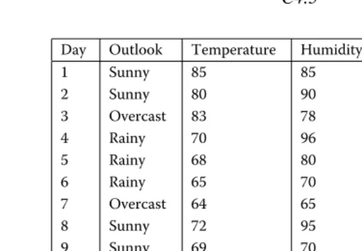
Figure 1.1 Example dataset input to C4.5.
(also continuous-valued), and Windy (binary), and the class is the Boolean PlayGolf? class variable. All of the data in Figure 1.1 constitutes “training data,” so that the intent is to learn a mapping using this dataset and apply it on other, new instances that present values for only the attributes to predict the value for the class random variable.
1.2 Algorithm Description 3
of ID3 and C4.5. Today, C4.5 is superseded by the See5/C5.0 system, a commercial product offered by Rulequest Research, Inc.
The fact that two of the top 10 algorithms are tree-based algorithms attests to the widespread popularity of such methods in data mining. Original applications of decision trees were in domains with nominal valued or categorical data but today they span a multitude of domains with numeric, symbolic, and mixed-type attributes. Examples include clinical decision making, manufacturing, document analysis, bio-informatics, spatial data modeling (geographic information systems), and practically any domain where decision boundaries between classes can be captured in terms of tree-like decompositions or regions identified by rules.
1.2
Algorithm Description
C4.5 is not one algorithm but rather a suite of algorithms—C4.5, C4.5-no-pruning, and C4.5-rules—with many features. We present the basic C4.5 algorithm first and the special features later.
The generic description of how C4.5 works is shown in Algorithm 1.1. All tree induction methods begin with a root node that represents the entire, given dataset and recursively split the data into smaller subsets by testing for a given attribute at each node. The subtrees denote the partitions of the original dataset that satisfy specified attribute value tests. This process typically continues until the subsets are “pure,” that is, all instances in the subset fall in the same class, at which time the tree growing is terminated.
Algorithm 1.1 C4.5(D)
Input: an attribute-valued dataset D
1: Tree ={}
2: if D is “pure” OR other stopping criteria met then
3: terminate
4: end if
5: for all attribute a∈ D do
6: Compute information-theoretic criteria if we split on a
7: end for
8: abest= Best attribute according to above computed criteria
9: Tree = Create a decision node that tests abestin the root
10: Dv= Induced sub-datasets from D based on abest
11: for all Dvdo
12: Treev= C4.5(Dv)
13: Attach Treevto the corresponding branch of Tree
14: end for
Yes
Yes
Yes
No No
Outlook
Humidity Windy
Sunny Rainy
Overcast
>75
[image:4.612.121.330.42.245.2]<=75 True False
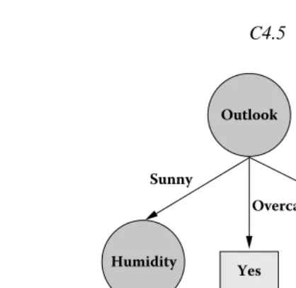
Figure 1.2 Decision tree induced by C4.5 for the dataset of Figure 1.1.
Figure 1.1 presents the classical “golf” dataset, which is bundled with the C4.5 installation. As stated earlier, the goal is to predict whether the weather conditions on a particular day are conducive to playing golf. Recall that some of the features are continuous-valued while others are categorical.
Figure 1.2 illustrates the tree induced by C4.5 using Figure 1.1 as training data (and the default options). Let us look at the various choices involved in inducing such trees from the data.
r What types of tests are possible? As Figure 1.2 shows, C4.5 is not restricted
to considering binary tests, and allows tests with two or more outcomes. If the attribute is Boolean, the test induces two branches. If the attribute is categorical, the test is multivalued, but different values can be grouped into a smaller set of options with one class predicted for each option. If the attribute is numerical,
then the tests are again binary-valued, and of the form{≤θ?, > θ?}, whereθ
is a suitably determined threshold for that attribute.
r How are tests chosen? C4.5 uses information-theoretic criteria such as gain
(reduction in entropy of the class distribution due to applying a test) and gain ratio (a way to correct for the tendency of gain to favor tests with many outcomes). The default criterion is gain ratio. At each point in the tree-growing, the test with the best criteria is greedily chosen.
r How are test thresholds chosen? As stated earlier, for Boolean and categorical
attributes, the test values are simply the different possible instantiations of that attribute. For numerical attributes, the threshold is obtained by sorting on that attribute and choosing the split between successive values that maximize the criteria above. Fayyad and Irani [10] showed that not all successive values need
1.2 Algorithm Description 5
attribute, if all instances involvingviand all instances involvingvi+1belong to
the same class, then splitting between them cannot possibly improve informa-tion gain (or gain ratio).
r How is tree-growing terminated? A branch from a node is declared to lead
to a leaf if all instances that are covered by that branch are pure. Another way in which tree-growing is terminated is if the number of instances falls below a specified threshold.
r How are class labels assigned to the leaves? The majority class of the instances
assigned to the leaf is taken to be the class prediction of that subbranch of the tree.
The above questions are faced by any classification approach modeled after trees and similar, or other reasonable, decisions are made by most tree induction algorithms. The practical utility of C4.5, however, comes from the next set of features that build upon the basic tree induction algorithm above. But before we present these features, it is instructive to instantiate Algorithm 1.1 for a simple dataset such as shown in Figure 1.1.
We will work out in some detail how the tree of Figure 1.2 is induced from Figure 1.1. Observe how the first attribute chosen for a decision test is the Outlook attribute. To see why, let us first estimate the entropy of the class random variable (PlayGolf?). This variable takes two values with probability 9/14 (for “Yes”) and 5/14 (for “No”). The entropy of a class random variable that takes on c values with probabilities p1,p2, . . . ,pcis given by:
c
i=1
−pilog2pi
The entropy of PlayGolf? is thus
−(9/14) log2(9/14)−(5/14) log2(5/14)
or 0.940. This means that on average 0.940 bits must be transmitted to communicate information about the PlayGolf? random variable. The goal of C4.5 tree induction is to ask the right questions so that this entropy is reduced. We consider each attribute in turn to assess the improvement in entropy that it affords. For a given random variable, say Outlook, the improvement in entropy, represented as Gain(Outlook), is calculated as:
Entropy(PlayGolf? in D)−
v
|Dv|
|D|Entropy(PlayGolf? in Dv)
wherevis the set of possible values (in this case, three values for Outlook), D denotes
the entire dataset, Dvis the subset of the dataset for which attribute Outlook has that
value, and the notation| · |denotes the size of a dataset (in the number of instances).
This calculation will show that Gain(Outlook) is 0.940−0.694=0.246. Similarly,
we can calculate that Gain(Windy) is 0.940−0.892=0.048. Working out the above
the best attribute to branch on. Observe that this is a greedy choice and does not take into account the effect of future decisions. As stated earlier, the tree-growing continues till termination criteria such as purity of subdatasets are met. In the above example, branching on the value “Overcast” for Outlook results in a pure dataset, that is, all instances having this value for Outlook have the value “Yes” for the class variable PlayGolf?; hence, the tree is not grown further in that direction. However, the other two values for Outlook still induce impure datasets. Therefore the algorithm recurses, but observe that Outlook cannot be chosen again (why?). For different branches, different test criteria and splits are chosen, although, in general, duplication of subtrees can possibly occur for other datasets.
We mentioned earlier that the default splitting criterion is actually the gain ratio, not the gain. To understand the difference, assume we treated the Day column in Figure 1.1 as if it were a “real” feature. Furthermore, assume that we treat it as a nominal valued attribute. Of course, each day is unique, so Day is really not a useful attribute to branch on. Nevertheless, because there are 14 distinct values for Day and each of them induces a “pure” dataset (a trivial dataset involving only one instance), Day would be unfairly selected as the best attribute to branch on. Because information gain favors attributes that contain a large number of values, Quinlan proposed the gain ratio as a correction to account for this effect. The gain ratio for an attribute a is defined as:
GainRatio(a)= Gain(a)
Entropy(a)
Observe that entropy(a) does not depend on the class information and simply takes into account the distribution of possible values for attribute a, whereas gain(a) does take into account the class information. (Also, recall that all calculations here are dependent on the dataset used, although we haven’t made this explicit in the notation.)
For instance, GainRatio(Outlook)=0.246/1.577=0.156. Similarly, the gain ratio
for the other attributes can be calculated. We leave it as an exercise to the reader to see if Outlook will again be chosen to form the root decision test.
1.3 C4.5 Features 7
1.3
C4.5 Features
1.3.1
Tree Pruning
Tree pruning is necessary to avoid overfitting the data. To drive this point, Quinlan gives a dramatic example in [30] of a dataset with 10 Boolean attributes, each of which assumes values 0 or 1 with equal accuracy. The class values were also binary: “yes” with probability 0.25 and “no” with probability 0.75. From a starting set of 1,000 instances, 500 were used for training and the remaining 500 were used for testing. Quinlan observes that C4.5 produces a tree involving 119 nodes (!) with an error rate of more than 35% when a simpler tree would have sufficed to achieve a greater accuracy. Tree pruning is hence critical to improve accuracy of the classifier on unseen instances. It is typically carried out after the tree is fully grown, and in a bottom-up manner.
The 1986 MIT AI lab memo authored by Quinlan [26] outlines the various choices available for tree pruning in the context of past research. The CART algorithm uses what is known as cost-complexity pruning where a series of trees are grown, each obtained from the previous by replacing one or more subtrees with a leaf. The last tree in the series comprises just a single leaf that predicts a specific class. The cost-complexity is a metric that decides which subtrees should be replaced by a leaf predicting the best class value. Each of the trees are then evaluated on a separate test dataset, and based on reliability measures derived from performance on the test dataset, a “best” tree is selected.
Reduced error pruning is a simplification of this approach. As before, it uses a separate test dataset but it directly uses the fully induced tree to classify instances in the test dataset. For every nonleaf subtree in the induced tree, this strategy evaluates whether it is beneficial to replace the subtree by the best possible leaf. If the pruned tree would indeed give an equal or smaller number of errors than the unpruned tree and the replaced subtree does not itself contain another subtree with the same property, then the subtree is replaced. This process is continued until further replacements actually increase the error over the test dataset.
Pessimistic pruning is an innovation in C4.5 that does not require a separate test set. Rather it estimates the error that might occur based on the amount of misclassifications in the training set. This approach recursively estimates the error rate associated with a node based on the estimated error rates of its branches. For a leaf with N instances and E errors (i.e., the number of instances that do not belong to the class predicted by that leaf), pessimistic pruning first determines the empirical error rate at the leaf
as the ratio (E+0.5)/N . For a subtree with L leaves andE andN corresponding
errors and number of instances over these leaves, the error rate for the entire subtree
is estimated to be (E+0.5∗L)/N . Now, assume that the subtree is replaced by
its best leaf and that J is the number of cases from the training set that it misclassifies.
Pessimistic pruning replaces the subtree with this best leaf if ( J+0.5) is within one
standard deviation of (E+0.5∗L).
Leaf predicting most likely class X1 X2 X3
T1 T2 T3
X
X1 X2 X3
T1 T2
T2
[image:8.612.137.313.58.210.2]T3 X
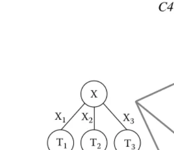
Figure 1.3 Different choices in pruning decision trees. The tree on the left can be retained as it is or replaced by just one of its subtrees or by a single leaf.
a given confidence threshold C I , an upper bound emaxcan be determined such that
e<emaxwith probability 1−C I . (C4.5 uses a default CI of 0.25.) We can go even
further and approximate e by the normal distribution (for large N ), in which case C4.5 determines an upper bound on the expected error as:
e+2Nz2 +z
e
N −
e2
N +
z2
4N2
1+zN2 (1.1)
where z is chosen based on the desired confidence interval for the estimation, assuming
a normal random variable with zero mean and unit variance, that is,N(0,1)).
What remains to be presented is the exact way in which the pruning is performed. A single bottom-up pass is performed. Consider Figure 1.3, which depicts the pruning
process midway so that pruning has already been performed on subtrees T1, T2, and
T3. The error rates are estimated for three cases as shown in Figure 1.3 (right). The
first case is to keep the tree as it is. The second case is to retain only the subtree corresponding to the most frequent outcome of X (in this case, the middle branch). The third case is to just have a leaf labeled with the most frequent class in the training dataset. These considerations are continued bottom-up till we reach the root of the tree.
1.3.2
Improved Use of Continuous Attributes
1.3 C4.5 Features 9
instances nearly equally, then the gain ratio is minimal (since the entropy of the vari-able falls in the denominator). Therefore, Quinlan advocates going back to the regular information gain for choosing a threshold but continuing the use of the gain ratio for choosing the attribute in the first place. A second approach is based on Risannen’s MDL (minimum description length) principle. By viewing trees as theories, Quinlan proposes trading off the complexity of a tree versus its performance. In particular, the complexity is calculated as both the cost of encoding the tree plus the exceptions to the tree (i.e., the training instances that are not supported by the tree). Empirical tests show that this approach does not unduly favor continuous-valued attributes.
1.3.3
Handling Missing Values
Missing attribute values require special accommodations both in the learning phase and in subsequent classification of new instances. Quinlan [28] offers a comprehen-sive overview of the variety of issues that must be considered. As stated therein, there are three main issues: (i) When comparing attributes to branch on, some of which have missing values for some instances, how should we choose an appropriate split-ting attribute? (ii) After a splitsplit-ting attribute for the decision test is selected, training instances with missing values cannot be associated with any outcome of the decision test. This association is necessary in order to continue the tree-growing procedure. Therefore, the second question is: How should such instances be treated when dividing the dataset into subdatasets? (iii) Finally, when the tree is used to classify a new in-stance, how do we proceed down a tree when the tree tests on an attribute whose value is missing for this new instance? Observe that the first two issues involve learning/ inducing the tree whereas the third issue involves applying the learned tree on new instances. As can be expected, there are several possibilities for each of these ques-tions. In [28], Quinlan presents a multitude of choices for each of the above three issues so that an integrated approach to handle missing values can be obtained by specific instantiations of solutions to each of the above issues. Quinlan presents a coding scheme in [28] to design a combinatorial strategy for handling missing values. For the first issue of evaluating decision tree criteria based on an attribute a, we can: (I) ignore cases in the training data that have a missing value for a; (C) substitute the most common value (for binary and categorical attributes) or by the mean of the known values (for numeric attributes); (R) discount the gain/gain ratio for attribute a by the proportion of instances that have missing values for a; or (S) “fill in” the missing value in the training data. This can be done either by treating them as a distinct, new value, or by methods that attempt to determine the missing value based on the values of other known attributes [28]. The idea of surrogate splits in CART (see Chapter 10) can be viewed as one way to implement this last idea.
the tree for cases with missing values for a; or (S) determine the most likely value of a (as before, using methods referenced in [28]) and assign it to the corresponding subdataset. In [28], Quinlan offers a variation on (F) as well, where the instance is assigned to only one subdataset but again proportionally to the number of instances with known values in that subdataset.
Finally, when classifying instances with missing values for attribute a, the options are: (U) if there is a separate branch for unknown values for a, follow the branch; (C) branch on the most common value for a; (S) apply the test as before from [28] to determine the most likely value of a and branch on it; (F) explore all branchs simul-taneously, combining their results to denote the relative probabilities of the different outcomes [27]; or (H) terminate and assign the instance to the most likely class.
As the reader might have guessed, some combinations are more natural, and other combinations do not make sense. For the proportional assignment options, as long as the weights add up to 1, there is a natural way to generalize the calculations of information gain and gain ratio.
1.3.4
Inducing Rulesets
A distinctive feature of C4.5 is its ability to prune based on rules derived from the induced tree. We can model a tree as a disjunctive combination of conjunctive rules, where each rule corresponds to a path in the tree from the root to a leaf. The antecedents in the rule are the decision conditions along the path and the consequent is the predicted class label. For each class in the dataset, C4.5 first forms rulesets from the (unpruned) tree. Then, for each rule, it performs a hill-climbing search to see if any of the antecedents can be removed. Since the removal of antecedents is akin to “knocking out” nodes in an induced decision tree, C4.5’s pessimistic pruning methods are used here. A subset of the simplified rules is selected for each class. Here the minimum description length (MDL) principle is used to codify the cost of the theory involved in encoding the rules and to rank the potential rules. The number of resulting rules is typically much smaller than the number of leaves (paths) in the original tree. Also observe that because all antecedents are considered for removal, even nodes near the top of the tree might be pruned away and the resulting rules may not be compressible back into one compact tree. One disadvantage of C4.5 rulesets is that they are known to cause rapid increases in learning time with increases in the size of the dataset.
1.4
Discussion on Available Software Implementations
1.5 Two Illustrative Examples 11
part of SGI’s Mineset data mining suite, and the Weka [35] data mining suite from the University of Waikato, New Zealand (http://www.cs.waikato.ac.nz/ml/weka/). The (Java) implementation of C4.5 in Weka is referred to as J48. Commercial implemen-tations of C4.5 include ODBCMINE from Intelligent Systems Research, LLC, which interfaces with ODBC databases and Rulequest’s See5/C5.0, which improves upon C4.5 in many ways and which also comes with support for ODBC connectivity.
1.5
Two Illustrative Examples
1.5.1
Golf Dataset
We describe in detail the function of C4.5 on the golf dataset. When run with the default options, that is:
>c4.5 -f golf
C4.5 produces the following output:
C4.5 [release 8] decision tree generator Wed Apr 16 09:33:21 2008
---Options:
File stem <golf>
Read 14 cases (4 attributes) from golf.data
Decision Tree:
outlook = overcast: Play (4.0) outlook = sunny:
| humidity <= 75 : Play (2.0)
| humidity > 75 : Don't Play (3.0)
outlook = rain:
| windy = true: Don't Play (2.0)
| windy = false: Play (3.0)
Tree saved
Evaluation on training data (14 items):
Before Pruning After Pruning
---
---Size Errors Size Errors Estimate
Referring back to the output from C4.5, observe the statistics presented toward the end of the run. They show the size of the tree (in terms of the number of nodes, where both internal nodes and leaves are counted) before and after pruning. The error over the training dataset is shown for both the unpruned and pruned trees as is the estimated error after pruning. In this case, as is observed, no pruning is performed.
The-voption for C4.5 increases the verbosity level and provides detailed,
step-by-step information about the gain calculations. Thec4.5rulessoftware uses similar
options but generates rules with possible postpruning, as described earlier. For the golf dataset, no pruning happens with the default options and hence four rules are output (corresponding to all but one of the paths of Figure 1.2) along with a default rule.
The induced trees and rules must then be applied on an unseen “test” dataset to
assess its generalization performance. The-uoption of C4.5 allows the provision of
test data to evaluate the performance of the induced trees/rules.
1.5.2
Soybean Dataset
Michalski’s Soybean dataset is a classical machine learning test dataset from the UCI Machine Learning Repository [3]. There are 307 instances with 35 attributes and many missing values. From the description in the UCI site:
There are 19 classes, only the first 15 of which have been used in prior work. The folklore seems to be that the last four classes are unjustified by the data since they have so few examples. There are 35 categorical attributes, some nominal and some ordered. The value “dna” means does not apply. The values for attributes are encoded numerically, with the first value encoded as “0,” the second as “1,” and so forth. An unknown value is encoded as “?.”
The goal of learning from this dataset is to aid soybean disease diagnosis based on observed morphological features.
The induced tree is too complex to be illustrated here; hence, we depict the evalu-ation of the tree size and performance before and after pruning:
Before Pruning After Pruning
--- ---Size Errors Size Errors Estimate
177 15( 2.2%) 105 26( 3.8%) (15.5%) <<
1.6 Advanced Topics 13
1.6
Advanced Topics
With the massive data emphasis of modern data mining, many interesting research issues in mining tree/rule-based classifiers have come to the forefront. Some are covered here and some are described in the exercises. Proceedings of conferences such as KDD, ICDM, ICML, and SDM showcase the latest in many of these areas.
1.6.1
Mining from Secondary Storage
Modern datasets studied in the KDD community do not fit into main memory and hence implementations of machine learning algorithms have to be completely rethought in order to be able to process data from secondary storage. In particular, algorithms are designed to minimize the number of passes necessary for inducing a classifer. The BOAT algorithm [14] is based on bootstrapping. Beginning from a small in-memory subset of the original dataset, it uses sampling to create many trees, which are then overlaid on top of each other to obtain a tree with “coarse” splitting criteria. This tree is then refined into the final classifier by conducting one complete scan over the dataset. The Rainforest framework [15] is an integrated approach to instantiate various choices of decision tree construction and apply them in a scalable manner to massive datasets. Other algorithms aimed at mining from secondary storage are SLIQ [21], SPRINT [34], and PUBLIC [33].
1.6.2
Oblique Decision Trees
An oblique decision tree, suitable for continuous-valued data, is so named because its decision boundaries can be arbitrarily positioned and angled with respect to the coordinate axes (see also Exercise 2 later). For instance, instead of a decision criterion
such as a1≤6? on attribute a1, we might utilize a criterion based on two attributes in
a single node, such as 3a1−2a2 ≤6? A classic reference on decision trees that use
linear combinations of attributes is the OC1 system described in Murthy, Kasif, and Salzberg [22], which acknowledges CART as an important basis for OC1. The basic idea is to begin with an axis-parallel split and then “perturb” it in order to arrive at a better split. This is done by first casting the axis-parallel split as a linear combination of attribute values and then iteratively adjusting the coefficients of the linear combination to arrive at a better decision criterion. Needless to say, issues such as error estimation, pruning, and handling missing values have to be revisited in this context. OC1 is a careful combination of hill climbing and randomization to tweaking the coefficients. Other approaches to inducing oblique decision trees are covered in, for instance, [5].
1.6.3
Feature Selection
irrelevant to predicting the given class and still other features could be redundant given other features. Feature selection is the idea of narrowing down on a smaller set of features for use in induction. Some feature selection methods work in concert with specific learning algorithms whereas methods such as described in Koller and Sahami [18] are learning algorithm-agnostic.
1.6.4
Ensemble Methods
Ensemble methods have become a mainstay in the machine learning and data mining literature. Bagging and boosting (see Chapter 7) are popular choices. Bagging is based on random resampling, with replacement, from the training data, and inducing one tree from each sample. The predictions of the trees are then combined into one output, for example, by voting. In boosting [12], as studied in Chapter 7, we generate a series of classifiers, where the training data for one is dependent on the classifier from the pre-vious step. In particular, instances incorrectly predicted by the classifier in a given step are weighted more in the next step. The final prediction is again derived from an aggre-gate of the predictions of the individual classifiers. The C5.0 system supports a variant of boosting, where an ensemble of classifiers is constructed and which then vote to yield the final classification. Opitz and Maclin [23] present a comparison of ensemble methods for decision trees as well as neural networks. Dietterich [8] presents a com-parison of these methods with each other and with “randomization,” where the internal decisions made by the learning algorithm are themselves randomized. The alternating decision tree algorithm [11] couples tree-growing and boosting in a tighter manner: In addition to the nodes that test for conditions, an alternating decision tree introduces “prediction nodes” that add to a score that is computed alongside the path from the root to a leaf. Experimental results show that it is as robust as boosted decision trees.
1.6.5
Classification Rules
1.7 Exercises 15
The descriptive line of research originates from association rules, a popular tech-nique in the KDD community [1, 2] (see Chapter 4). Traditionally, associations are
between two sets, X and Y , of items, denoted by X →Y , and evaluated by measures
such as support (the fraction of instances in the dataset that have both X and Y ) and confidence (the fraction of instances with X that also have Y ). The goal of associ-ation rule mining is to find all associassoci-ations satisfying given support and confidence thresholds. CBA (Classification based on Association Rules) [20] is an adaptation of association rules to classification, where the goal is to determine all association rules that have a certain class label in the consequent. These rules are then used to build a classifier. Pruning is done similarly to error estimation methods in C4.5. The key difference between CBA and C4.5 is the exhaustive search for all possible rules and efficient algorithms adapted from association rule mining to mine rules. This thread of research is now an active one in the KDD community with new variants and applications.
1.6.6
Redescriptions
Redescriptions are a generalization of rules to equivalences, introduced in [32]. As the name indicates, to redescribe something is to describe anew or to express the same concept in a different vocabulary. Given a vocabulary of descriptors, the goal of redescription mining is to construct two expressions from the vocabulary that induce the same subset of objects. The underlying premise is that sets that can indeed be defined in (at least) two ways are likely to exhibit concerted behavior and are, hence, interesting. The CARTwheels algorithm for mining redescriptions grows two C4.5-like trees in opposite directions such that they are matched at the leaves. Essentially, one tree exposes a partition of objects via its choice of subsets and the other tree tries to grow to match this partition using a different choice of subsets. If partition correspondence is established, then paths that join can be read off as redescriptions. CARTwheels explores the space of possible tree matchings via an alternation process whereby trees are repeatedly regrown to match the partitions exposed by the other tree. Redescription mining has since been generalized in many directions [19, 24, 37].
1.7
Exercises
1. Carefully quantify the big-Oh time complexity of decision tree induction with C4.5. Describe the complexity in terms of the number of attributes and the number of training instances. First, bound the depth of the tree and then cast the time required to build the tree in terms of this bound. Assess the cost of pruning as well.
axes. Apply C4.5 on this dataset and comment on the quality of the induced trees. Take factors such as accuracy, size of the tree, and comprehensibility into account.
3. An alternative way to avoid overfitting is to restrict the growth of the tree rather than pruning back a fully grown tree down to a reduced size. Explain why such prepruning may not be a good idea.
4. Prove that the impurity measure used by C45 (i.e., entropy) is concave. Why is it important that it be concave?
5. Derive Equation (1.1). As stated in the text, use the normal approximation to the Bernoulli random variable modeling the error rate.
6. Instead of using information gain, study how decision tree induction would be affected if we directly selected the attribute with the highest prediction accuracy. Furthermore, what if we induced rules with only one antecedent? Hint: You are retracing the experiments of Robert Holte as described in R. Holte, Very Simple Classification Rules Perform Well on Most Commonly Used Datasets, Machine Learning, vol. 11, pp. 63–91, 1993.
7. In some machine learning applications, attributes are set-valued, for example, an object can have multiple colors and to classify the object it might be important to model color as a set-valued attribute rather than as an instance-valued attribute. Identify decision tests that can be performed on set-valued attributes and explain which can be readily incorporated into the C4.5 system for growing decision trees.
8. Instead of classifying an instance into a single class, assume our goal is to obtain a ranking of classes according to the (posterior) probability of membership of the instance in various classes. Read F. Provost and P. Domingos, Tree Induction for Probability Based Ranking, Machine Learning, vol. 52, no. 3, pp. 199–215, 2003, who explain why the trees induced by C4.5 are not suited to providing reliable probability estimates; they also suggest some ways to fix this problem using probability smoothing methods. Do these same objections and solution strategy apply to C4.5 rules as well? Experiment with datasets from the UCI repository.
9. (Adapted from S. Nijssen and E. Fromont, Mining Optimal Decision Trees from Itemset Lattices, Proceedings of the 13th ACM SIGKDD International Conference on Knowledge Discovery and Data Mining, pp. 530–539, 2007.) The trees induced by C4.5 are driven by heuristic choices but assume that our goal is to identify an optimal tree. Optimality can be posed in terms of various considerations; two such considerations are the most accurate tree up to a certain maximum depth and the smallest tree in which each leaf covers at least k instances and the expected accuracy is maximized over unseen examples. Describe an efficient algorithm to induce such optimal trees.
References 17
first-order features. Your solution must allow the induction of trees or rules of the form:
grandparent(X,Z) :- parent(X,Y), parent(Y,Z).
that is, Xis a grandparent ofZif there existsYsuch thatYis the parent of
XandZis the parent ofY. Several new issues result from the choice of
first-order logic as the representational language. First, unlike the attribute value
situation, first-order features (such asparent(X,Y)) are not readily given
and must be generalized from the specific instances. Second, it is possible to obtain nonsensical trees or rules if the variables participate in the head of a rule but not the body, for example:
grandparent(X,Y) :- parent(X,Z).
Describe how you can place checks and balances into the induction process so that a complete first-order theory can be induced from data. Hint: You are exploring the field of inductive logic programming [9], specifically, algorithms such as FOIL [29].
References
[1] R. Agrawal, T. Imielinski, and A. N. Swami. Mining association rules between
sets of items in large databases. In Proceedings of the ACM SIGMOD Interna-tional Conference on Management of Data (SIGMOD’93), pp. 207–216, May 1993.
[2] R. Agrawal and R. Srikant. Fast algorithms for mining association rules in large
databases. In Proceedings of the 20th International Conference on Very Large Databases (VLDB’94), pp. 487–499, Sep. 1994.
[3] A. Asuncion and D. J. Newman. UCI Machine Learning Repository, 2007.
http://www.ics.uci.edu/∼mlearn/MLRepository.html. University of California, Irvine, School of Information and Computer Sciences.
[4] L. Breiman, J. Friedman, C. J. Stone, and R. A. Olshen. Classification and
Regression Trees. Chapman & Hall/CRC, Jan. 1984.
[5] C. E. Brodely and P. E. Utgoff. Multivariate Decision Trees. Machine Learning,
19:45–77, 1995.
[6] P. Clark and T. Niblett. The CN2 Induction Algorithm. Machine Learning,
3(4):261–283, 1999.
[7] W. Cohen. Fast Efficient Rule Induction. In Proceedings of the Twelfth
[8] T. G. Dietterich. An Experimental Comparison of Three Methods for Con-structing Ensembles of Decision Trees: Bagging, Boosting, and Randomiza-tion. Machine Learning, 40(2):139–157, 2000.
[9] S. Dzeroski and N. Lavrac, eds. Relational Data Mining. Springer, Berlin, 2001.
[10] U. M. Fayyad and K. B. Irani. On the Handling of Continuous-Valued Attributes
in Decision Tree Generation. Machine Learning, 8(1):87–102, Jan. 1992.
[11] Y. Freund and L. Mason. The Alternating Decision Tree Learning Algorithm.
In Proceedings of the Sixteenth International Conference on Machine Learning (ICML 1999), pp. 124–133, 1999.
[12] Y. Freund and R. E. Schapire. A Short Introduction to Boosting. Journal of the
Japanese Society for Artificial Intelligence, 14(5):771–780, Sep. 1999.
[13] J. H. Friedman. A Recursive Partitioning Decision Rule for Nonparametric
Classification. IEEE Transactions on Computers, 26(4):404–408, Apr. 1977.
[14] J. Gehrke, V. Ganti, R. Ramakrishnan, and W.-H. Loh. BOAT: Optimistic
De-cision Tree Construction. In Proceedings of the ACM SIGMOD International Conference on Management of Data (SIGMOD’99), pp. 169–180, 1999.
[15] J. Gehrke, R. Ramakrishnan, and V. Ganti. RainForest: A Framework for Fast
Decision Tree Construction of Large Datasets. Data Mining and Knowledge Discovery, 4(2/3):127–162, 2000.
[16] E. B. Hunt, J. Marin, and P. J. Stone. Experiments in Induction. Academic Press,
New York, 1966.
[17] R. Kohavi, D. Sommerfield, and J. Dougherty. Data Mining Using MLC++: A
Machine Learning Library in C++. In Proceedings of the Eighth International Conference on Tools with Artificial Intelligence (ICTAI ’96), pp. 234–245, 1996.
[18] D. Koller and M. Sahami. Toward Optimal Feature Selection. In Proceedings
of the Thirteenth International Conference on Machine Learning (ICML’96), pp. 284–292, 1996.
[19] D. Kumar, N. Ramakrishnan, R. F. Helm, and M. Potts. Algorithms for
Sto-rytelling. In Proceedings of the Twelfth ACM SIGKDD International Con-ference on Knowledge Discovery and Data Mining (KDD’06), pp. 604–610, Aug. 2006.
[20] B. Liu, W. Hsu, and Y. Ma. Integrating Classification and Association Rule
Mining. In Proceedings of the Fourth International Conference on Knowledge Discovery and Data Mining (KDD’98), pp. 80–86, Aug. 1998.
[21] M. Mehta, R. Agrawal, and J. Rissanen. SLIQ: A Fast Scalable Classifier for
Data Mining. In Proceedings of the 5th International Conference on Extending Database Technology (EDBT’96), pp. 18–32, Mar. 1996.
[22] S. K. Murthy, S. Kasif, and S. Salzberg. A System for Induction of Oblique
References 19
[23] D.W. Opitz and R. Maclin. Popular Ensemble Methods: An Empirical Study.
Journal of Artificial Intelligence Research, 11:169–198, 1999.
[24] L. Parida and N. Ramakrishnan. Redescription Mining: Structure Theory and
Algorithms. In Proceedings of the Twentieth National Conference on Artificial Intelligence (AAAI’05), pp. 837–844, July 2005.
[25] J. R. Quinlan. Induction of Decision Trees. Machine Learning, 1(1):81–106,
1986.
[26] J. R. Quinlan. Simplifying Decision Trees. Technical Report 930, MIT AI Lab
Memo, Dec. 1986.
[27] J. R. Quinlan. Decision Trees as Probabilistic Classifiers. In P. Langley, ed.,
Proceedings of the Fourth International Workshop on Machine Learning. Mor-gan Kaufmann, CA, 1987.
[28] J. R. Quinlan. Unknown Attribute Values in Induction. Technical report, Basser
Department of Computer Science, University of Sydney, 1989.
[29] J. R. Quinlan. Learning Logical Definitions from Relations. Machine Learning,
5:239–266, 1990.
[30] J. R. Quinlan. C4.5: Programs for Machine Learning. Morgan Kaufmann, 1993.
[31] J. R. Quinlan. Improved Use of Continuous Attributes in C4.5. Journal of
Artificial Intelligence Research, 4:77–90, 1996.
[32] N. Ramakrishnan, D. Kumar, B. Mishra, M. Potts, and R. F. Helm. Turning
CARTwheels: An Alternating Algorithm for Mining Redescriptions. In Pro-ceedings of the Tenth ACM SIGKDD International Conference on Knowledge Discovery and Data Mining (KDD’04), pp. 266–275, Aug. 2004.
[33] R. Rastogi and K. Shim. PUBLIC: A Decision Tree Classifier that Integrates
Building and Pruning. In Proceedings of the 24th International Conference on Very Large Data Bases (VLDB’98), pp. 404–415, Aug. 1998.
[34] J. C. Shafer, R. Agrawal, and M. Mehta. SPRINT: A Scalable Parallel Classifier
for Data Mining. In Proceedings of the 22th International Conference on Very Large Data Bases (VLDB’96), pp. 544–555, Sep. 1996.
[35] I. H. Witten and E. Frank. Data Mining: Practical Machine Learning Tools and
Techniques. Morgan Kaufmann, 2005.
[36] X. Wu, V. Kumar, J. R. Quinlan, J. Ghosh, Q. Yang, H. Motoda, G. J. McLachlan,
A. Ng, B. Liu, P. S. Yu, Z.-H. Zhou, M. Steinbach, D. J. Hand, and D. Steinberg. Top 10 Algorithms in Data Mining. Knowledge and Information Systems, 14:1–37, 2008.
[37] L. Zhao, M. Zaki, and N. Ramakrishnan. BLOSOM: A Framework for Mining