A simple test for the presence of multidomain behavior during paleointensity experiments

A simple test for the presence of multidomain

behavior during paleointensity experiments

Greig A. Paterson

Received 16 March 2011; revised 16 July 2011; accepted 21 July 2011; published 19 October 2011.

[1]

Detecting and excluding non

‐

ideal behavior during paleointensity experiments is

critical to asserting the reliability of data. Our knowledge of detecting non

‐

ideal behavior,

in particular the influence of multidomain (MD) grains, has expanded considerably

over the past decade and experimental procedures now commonly incorporate checks

to detect the effects of MD behavior. However, many older studies were carried out

before these checks were devised and provide no quantifiable means of testing for the

presence of MD grains. An estimated one third of all entries in the most recent

paleointensity database do not include some form of check for MD behavior. The

reliability of these results is therefore questionable and can only hinder efforts to

understand the evolution of the geomagnetic field and the geodynamo. I propose a simple

phenomenological check that can be applied to previous studies, provided that the raw data

are available, that will allow the exclusion of MD behavior and provide a means of

identifying reliable data. The check is a quantification of the curvature,

k

, of data points

on an Arai plot, a feature commonly associated with MD behavior. Analysis of

paleointensity data from samples with known grain size indicates that this new parameter

is significantly correlated with grain size and with the accuracy of the paleointensity

estimates made from both limbs of the curved data. Analysis of 181 samples from five

historical data sets indicates that

k

is significantly correlated with experimentally obtained

MD and alteration check parameters, and the accuracy of the paleointensity estimate.

A threshold selection value of

k

≤

0.164 can be defined using the samples with known

grain sizes. Applying this cut

‐

off value, combined with a threshold on the quality of

the circle fit and a commonly used alteration check, to the historical data yields an accurate

result with low scatter. When compared with previously published selection criteria

that incorporate experimental checks for non

‐

ideal behavior, the result of applying the

criteria proposed here is an improvement. The application of these three criteria rejects

over 65% of all inaccurate results and has the highest concentration of accurate results

when compared with the other criteria sets tested. Other selection criteria can be

subsequently used to improve on this result. While modern studies should always include

experimental checks to identify MD behavior, this new criterion will provide a useful tool

for future studies and, importantly, a method to assess the reliability of previously

published data.

Citation: Paterson, G. A. (2011), A simple test for the presence of multidomain behavior during paleointensity experiments,

J. Geophys. Res.,116, B10104, doi:10.1029/2011JB008369.

1.

Introduction

[2] Determining the strength of the paleomagnetic field from

geological materials can provide important constraints on our understanding of the evolution of the geodynamo, Earth’s core, and core‐mantle interactions. However, absolute

paleointen-sity experiments can be time consuming, difficult, and prone to high failure rates [e.g.,Riisager et al., 2002;Pan et al., 2005; Paterson et al., 2010b]. In the past decade or so, a number of advances have expanded our knowledge of the causes and effects of non‐ideal paleointensity behavior [McClelland and Briden, 1996;Valet et al., 1996;Riisager and Riisager, 2001;Selkin et al., 2000;Krása et al., 2003;Draeger et al., 2006; Yamamoto, 2006; Selkin et al., 2007; Fabian, 2009]. Some of these advances suggest the inclusion of additional experimental steps that allow the quantification, and some-times the correction of, non‐ideal behavior [e.g.,McClelland and Briden, 1996; Selkin et al., 2000; Krása et al., 2003].

1_{Paleomagnetism and Geochronology Laboratory, Key Laboratory of} Earth’s Deep Interior, Institute of Geology and Geophysics, Chinese Academy of Sciences, Beijing, China.

One result of the recent efforts to identify non‐ideal paleoin-tensity behavior is that, due to a lack of what are now becoming standard tests, many older data sets are deemed as unreliable and often discarded, or given a lower rank during meta‐analyses [e.g.,Selkin and Tauxe, 2000;Ziegler et al., 2008]. While some non‐ideal behavior can be tested for post‐experiment, with additional measurements (e.g., remanence anisotropy), others, such as the influence of multidomain (MD) grains and alteration during laboratory heating, cannot be directly tested.

[3] It is difficult to assess the number of studies that do

not include tests for MD behavior: To date no paleointensity database records this information. However, nearly one third of the entries in the current PINT database [Biggin, 2010] are from studies using Thellier‐type methods [Thellier and Thellier, 1959; Coe, 1967] published before the first sug-gestion of an experimental procedure that could test for MD effects [McClelland and Briden, 1996]. This is likely to be a minimum estimate as more than half of the entries were published before it was established that such a procedure could be used to detect MD effects [Riisager and Riisager, 2001]. The large proportion of paleointensity data that may be influenced by non‐ideal effects will undoubtedly hinder efforts to understand the long‐term variation of the geo-magnetic field. It is therefore essential to develop new analyses and criteria to assess the fidelity of paleointensity data from previously published studies.

[4] In this paper I propose a new phenomenological

cri-terion that quantifies curvature on an Arai plot and inves-tigates the manifestation of curvature due to the effects of MD grains. This new criterion does not require any addi-tional measurements and can be applied to Thellier‐type studies that use the Coe protocol, provided that the data required to construct an Arai plot [Nagata et al., 1963] are available. The criterion makes use of the well documented feature that pseudo‐single domain (PSD) and MD grains produce a curved sequence of points when plotted for analysis on an Arai plot [e.g.,Levi, 1977;Shcherbakov and Shcherbakova, 2001]. The source of this curvature can be attributed to magnetizations that are unblocked (demagne-tized) at temperatures below their respective blocking tem-peratures, which leads to an excess loss of remanence at

lower temperatures compared to remanence gained [Fabian, 2001; Leonhardt et al., 2004b] and due to the progressive stabilization of domain structures during the repeated heat-ings required during a Thellier‐type paleointensity experi-ment [Shcherbakov and Shcherbakova, 2001;Yu and Tauxe, 2006].

2.

Methods

2.1. Quantifying Curvature

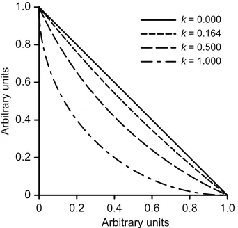
[5] Curvature is defined as the degree to which an object

(e.g., a line or a plane) deviates from being perfectly flat. In the case of a line, curvature is the reciprocal of the radius of curvature. To quantify the curvature of data on an Arai plot, a best‐fit circle of the form (x−a)2+ (y−b)2=r2is fitted to the data using a least squares approach [Taubin, 1991; Chernov and Lesort, 2005], where x represents the ther-moremanent magnetization (TRM) gained, andyrepresents the natural remanent magnetization (NRM) remaining. The best‐fit circle is not anchored to any point on the Arai plot. With this approach the data on an Arai plot represent an arc of a much larger circle. The curvature (k) of the circle can then be simply calculated as1_r. The higher the value ofkthe more curved the arc is (i.e., the smaller the circle), the lower the value ofkthe closer the arc is to being a straight line. For a perfectly straight line k ≡ 0. The quality of the best‐fit circle to the data can be assessed by determining the sum of the squares of the errors (SSE):

SSE¼X n

i¼1

ffiffiffiffiffiffiffiffiffiffiffiffiffiffiffiffiffiffiffiffiffiffiffiffiffiffiffiffiffiffiffiffiffiffiffiffiffiffiffiffiffiffi xia

ð Þ2þðyibÞ2

q

r

2

: ð1Þ

[6] Examples of arcs with different values ofkare shown

in Figure 1. In Figure 1 the segments of the circles that fall within the coordinate region of an Arai plot have been selected to illustrate the similarity between these circles and real paleointensity data. The appropriateness of fitting circle to paleointensity data is discussed in more detail in the auxiliary material.1

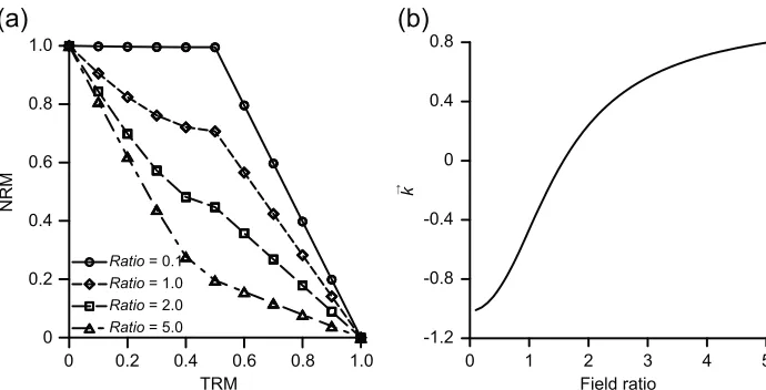
[7] To ensure an equal comparison of different samples

the data must be appropriately scaled. While normalizing both axes by the same constant, be it the maximum NRM or TRM, preserves the relative relationship for the calculation of the best linear fit, this type of normalization produces different values of k, which depend on the value of the normalization parameter. For example, if two identical and ideal samples recording the same paleointensity were sub-jected to identical intensity experiments, but with differing laboratory fields, normalization by the initial NRM would produce different TRM coordinates for each sample. This would result in different values ofkdespite the linearity of the data being identical. To ensure consistency each axis is normalized by the maximum value of the data on that axis such that 0≤ TRM≤1, and 0≤NRM≤1. For the calcu-lation ofkall data points on the Arai plot are used, not just those used to obtain the best linear fit. The implications of this are discussed further in section 6.

Figure 1. Schematic examples of the appearance of arcs with varying curvature (k).

1

2.2. Directionality of Curvature

[8] It should be noted that the definition ofkgiven above

only yields the absolute value ofk, that isk=1_r, wherer> 0. This does not, therefore, distinguish between curved data facing either up or down. When a best‐fit linear line is fitted to data, the best‐fit line passes through the centroid of the data (C= (x,y)). In the case of perfectly linear data the best‐

fit circle will also pass through Cwith r≡ ∞. As the data become more curved, in a concave‐up fashion, the centroid of the data will move above the data. For small degrees of curvature the center point of the circle (CP= (a,b)) will lie well aboveC, i.e.,x<aandy<b. For concave‐down data, the converse is true,a <xand b< y. In both cases, as the curvature increasesC will tend toCP, and for a circle that falls entirely within the plot C ≡ CP. Therefore, k can be

given a sign of direction to specify if the curvature is con-cave‐up or concave‐down based on the position of the center point of the best‐fit circle relative to the centroid of the data:

~k¼ 1

r if ðx<aÞand yð <bÞ

1

r if ða<xÞand bð <yÞ 0 ifða¼xÞand bð ¼yÞ 8

> > > > > < > > > > > :

ð2Þ

[9] Strictly, there are four possible directions of curvature,

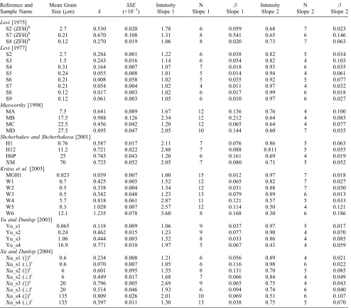
but the physical constraints of paleointensity data and analysis preclude the other two (i.e., all magnetizations must be greater than or equal to zero). Most Arai plots exhibit-ing MD‐like behavior data have concave‐up, or positive Table 1. Summary of the Grain Sizes and Analysis of the Synthetic Samplesa

Reference and Sample Name

Mean Grain

Size (mm) k

SSE

(×10−1₎ Intensity_{Slope 1 Slope 1}N _{Slope 1}b Intensity_{Slope 2 Slope 2}N _{Slope 2}b

Levi[1975]

S2 (ZFH)b 2.7 0.530 0.020 1.78 6 0.059 0.68 7 0.023

S7 (ZFH)b _{0.21 0.670 0.108 1.31 8 0.541 0.65 6 0.146}

S8 (ZFH)b 0.12 0.270 0.019 1.06 8 0.020 0.73 7 0.063

Levi[1977]

S2 2.7 0.284 0.001 1.22 6 0.038 0.82 5 0.034

S3 1.5 0.243 0.016 1.14 6 0.054 0.82 4 0.103

S4 0.31 0.164 0.007 1.07 7 0.018 0.93 6 0.035

S5 0.24 0.055 0.008 1.01 5 0.014 0.94 4 0.061

S6 0.21 0.008 0.058 1.02 5 0.035 0.92 5 0.077

S7 0.21 0.054 0.004 1.02 4 0.011 0.97 4 0.032

S8 0.12 0.017 0.003 1.02 6 0.017 0.99 6 0.018

S9 0.12 0.061 0.003 1.05 6 0.010 0.97 6 0.027

Muxworthy[1998]

MA 7.5 0.641 0.089 1.67 12 0.136 0.76 4 0.100

MB 17.5 0.988 0.126 2.34 12 0.212 0.64 4 0.085

MC 22.5 0.456 0.042 1.20 12 0.065 0.64 4 0.077

MD 27.5 0.895 0.047 2.05 10 0.144 0.60 7 0.035

Shcherbakov and Shcherbakova[2001]

H1 0.76 0.587 0.017 2.11 7 0.076 0.86 5 0.063

H12 11.2 0.721 0.022 2.88 7 0.088 0.811 5 0.055

H6P 25 0.743 0.043 1.20 6 0.161 0.69 4 0.019

XM 70 0.725 0.052 2.05 7 0.080 0.71 5 0.052

Krása et al.[2003]

MGH1 0.023 0.039 0.007 1.00 15 0.012 0.97 7 0.018

W1 0.7 0.425 0.005 1.52 12 0.065 0.82 7 0.027

W2 0.5 0.338 0.004 1.34 12 0.031 0.88 7 0.030

W3 0.5 0.342 0.048 1.23 13 0.079 0.89 6 0.013

W4 5.7 0.818 0.061 2.87 11 0.121 0.57 5 0.033

W5 8.3 1.028 0.007 2.57 12 0.114 0.50 4 0.121

W6 12.1 1.235 0.078 3.60 8 0.168 0.30 6 0.186

Yu and Dunlop[2003]

Yu_s1 0.065 0.118 0.009 1.06 9 0.037 0.97 5 0.017

Yu_s2 0.24 0.462 0.015 1.23 9 0.077 0.90 4 0.070

Yu_s3 1.06 0.444 0.003 1.52 8 0.033 0.86 4 0.085

Yu_s4 16.9 0.771 0.010 1.97 5 0.067 0.43 4 0.059

Xu and Dunlop[2004]

Xu_s1 (k)c 0.6 0.234 0.008 1.21 6 0.056 0.89 4 0.021

Xu_s1 (?)c _{0.6 0.070 0.007 1.05 6 0.116 0.98 6 0.022}

Xu_s2 (k)c 6 0.601 0.095 1.55 8 0.131 0.70 5 0.085

Xu_s2 (?)c _{6 0.449 0.017 1.68 7 0.066 0.84 4 0.049}

Xu_s3 (k)c 20 0.796 0.005 2.69 9 0.065 0.75 4 0.043

Xu_s3 (?)c _{20 0.514 0.046 1.93 6 0.094 0.74 6 0.040}

Xu_s4 (k)c 135 0.809 0.026 2.01 10 0.069 0.51 6 0.107

Xu_s4 (?)c 135 0.397 0.011 1.30 13 0.038 0.75 5 0.070

a_{Slope 1 and slope 2 refer to the low‐and high‐temperature segments, respectively. N refers to the number of points used to determine the best linear fit.} b

curvature [e.g.,Levi, 1977]. There are a number of reasons why data may have negative curvature, for example, small deviations from near perfectly linear data can produce low values of~k that are negative. Other causes, such as multi-component magnetizations, high‐temperature alteration, or generally noisy data are discussed in section 6. When dis-criminating against the effects of MD grains, or non‐linear

data in general, the magnitude of curvature, k= |~kj, is the important parameter; the direction of curvature can give some indication as to the cause of the non‐linear behavior.

3.

Application to Synthetic Samples

[10] Paleointensity data from various studies using

extracted natural and synthetic magnetite with known grain sizes have been compiled for this study and a summary of the samples used is given in Table 1. Although these sam-ples contain both natural and synthetic magnetite, for this study these samples will be collectively referred to as syn-thetic samples. Detailed descriptions of the samples and the experimental procedures are given in the respective refer-ences [Levi, 1975, 1977;Muxworthy, 1998;Shcherbakov and Shcherbakova, 2001;Krása et al., 2003;Yu and Dunlop, 2003;Xu and Dunlop, 2004, and references therein]. Prior to the paleointensity experiments all of the samples under-went thermal stabilization, typically being heated and held at high temperature (∼700°C) for a period of time (3+ h) to reduce the degree of stress within individual grains and to ensure no or little alteration during the proceeding expe-riments. All samples have be characterized as low‐Ti tita-nomagnetite (Ti ≈ 0–0.1%) based on Curie temperatures (565–586°C). BothMuxworthy[1998] andKrása et al.[2003] noted that the samples used in their studies may have a small degree of maghemitization. Examples of the Arai plots from these samples are shown in Figure 2 and all of the Arai plots are given in the auxiliary material. The paleo-intensity experiments performed on these samples were var-iants of the Coe double heating protocol [Coe, 1967]. In most experiments the laboratory field was applied parallel to the NRM, however, Xu and Dunlop [2004] also carried out experiments in which the applied the field was perpendicular to the NRM. Levi [1975] compared the effects of heating in zero field (zero field heating, ZFH) and heating in‐field (field heating, FH) during the partial TRM (pTRM) acquisition steps. The data therefore represent a wide variety of experi-mental conditions. Sample S11 fromLevi[1977] has not been included in this study due to the highly elongated shape of the magnetite crystals, which makes it difficult to compare with other grain sizes.

[11] Visually (Figure 2 and Figures S1–S7 in the auxiliary

material) and quantitatively (using the SSE, Table 1) the best‐fit arcs shown in Figure 2 fit the data well, with all values of theSSE≤0.0126 (Table 1). This is an indication that least squares circle fitting is appropriate for Arai plot data. All of the samples have positive curvature with k ranging from 0.008 to 1.235 (Table 1).

[12] To assess the accuracy of these samples at recording

paleointensities, best‐fit linear lines were fitted through two segments of the unnormalized data, one through the first several points and another through the last several points. These fits are referred to as the low‐temperature and high‐ temperature fits, respectively, after the experimental tem-peratures from which the data are obtained. Each fit consists of at least four consecutive data points and is fitted to the best linear section irrespective of the quality of fit, that is, for some fits the ratio of the standard error of the slope to the value of the slope (b) is higher than is typically accepted in many paleointensity studies (i.e.,b > 0.1). For a consis-tent comparison of the results from different samples the Figure 2. Example Arai plots from (a)Levi[1975], (b)Levi

paleointensity estimates are normalized by the expected values; hereafter simply referred to as the intensity estimate. To assess the accuracy of the intensity estimate the loga-rithm of the estimate was used in the analysis. When accuracy values are zeros the intensity estimate is exactly the expected value; positive and negative values represent over‐and underestimates, respectively. Results of the linear fitting are summarized in Table 1 and samples are consi-dered to yield an accurate estimate if the intensity estimate is within a factor 1.1 (10%) of the expected value (i.e., log (1/1.1)≤ log(Intensity)≤ log(1.1)). The paleointensity esti-mates from the synthetic samples are asymmetric in that the low‐temperature segments typically overestimate the expected intensity more than the high‐temperature segments underes-timate the intensity. Despite the asymmetry of the paleoin-tensity estimates made from the low‐ and high‐temperature segments, the curvature on the Arai plots is symmetric as is evident from the goodness‐of‐fit of the circles, which are inherently symmetric. A full discussion reconciling these different symmetries is given in the auxiliary material.

[13] Three studies incorporated experimental checks for

MD behavior [Muxworthy, 1998;Krása et al., 2003;Yu and Dunlop, 2003]. Due to the laboratory field being parallel to the NRM the check values are generally low [cf. Yu and Tauxe, 2005], except where the data suffer from noise (e.g., sample MB). The additivity check ofKrása et al.[2003] is the only MD check parameter that is consistently correlated with the logarithm of grain size (inmm). With data from only 15 samples it is difficult to assess the efficacy of pTRM tail checks; additional data are required, measured with various angles of laboratory field, to adequately asses these com-monly used MD checks.

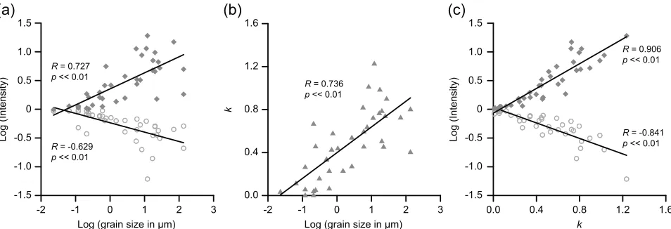
[14] As is expected, and commonly reported [e.g.,Chauvin

et al., 2005], paleointensity estimates from the low‐temperature segments overestimate the true intensity and estimates from the high‐temperature segments are underestimates (Table 1, Figure 3). A comparison between the accuracy of both segments and grain size indicates that the accuracies of both segments are significantly correlated with grain size (Figure 3a; unless otherwise stated correlations with grain size refer to

correla-tions with the logarithm of grain size). A comparison between curvature and grain size also yields a significant correlation (R= 0.736,p0.01), which confirms curved Arai plots are associated with large grains of magnetite (Figure 3b). Not only iskcorrelated with grain size, but it is also significantly correlated with the accuracy of the low‐temperature segment (R= 0.906, p 0.01) and with the accuracy of the high‐ temperature segment (R=−0.841,p0.01; Figure 3c). For a sample with constrained grain size kis a good proxy for grain size and the inaccuracies that larger grains can produce during a paleointensity experiment.

4.

Defining a Threshold for Data Selection

[15] Given the good correlations ofkwith grain size and

accuracy, can a threshold value be defined to exclude the effects of MD grains? Only two samples (MGH1 and Yu_s1) fall within the SD grain size range for magnetite (∼0.03 – ∼0.08 mm) [Dunlop and Özdemir, 1997]. These two samples have a maximum curvature of 0.118 (Table 1) and this may provide a suitable threshold value. It has been noted, however, that small PSD grains are capable of pro-ducing accurate results [Shcherbakov and Shcherbakova, 2001] and this is reaffirmed here (e.g., samples S4–9 and Xu_s1 (?), Table 1). Nine samples yield accurate intensity estimates from both segments and suggest a threshold value of k ≤ 0.164. One sample (S8 (ZFH)) yields an accurate estimate from one segment, but not both. This may suggest an upper maximum of k ∼ 0.270, but two samples yield inaccurate results with values ofkin this range (i.e., S3 and Xu_s3 (k)). Therefore a threshold value of k ≤ 0.164 is suggested to exclude inaccuracies produced by the effects of MD and large PSD grains. An example of the an arc with k= 0.164 is shown in Figure 1. The maximum grain size that passes this criterion is 0.6mm (Xu_s1 (?), Table 1).

5.

Application to Real Data

[16] To test the effectiveness ofkat excluding MD behavior

a paleointensity data set comprised of 181 estimates from five Figure 3. Paleointensity data from the synthetic samples. (a) Accuracy of the paleointensity estimates

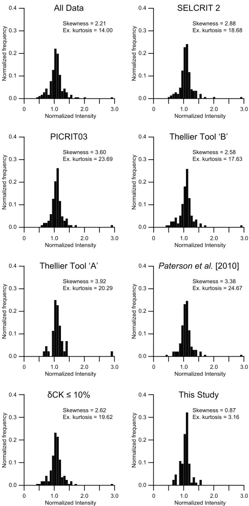
historical volcanoes, where the expected intensity of the geo-magnetic field is known from direct observations, was com-piled. The data set includes 18 data from the 1950, 1979, and 1983 eruption of Mt. Etna, Italy [Biggin et al., 2007], 52 data from the 1914 and 18 data from the 1946 eruption of Sakur-ajima, Japan [Yamamoto and Hoshi, 2008], 46 data from the 1993 eruption of Láscar, Chile [Paterson et al., 2010b], 29 data from the 1943 eruption of Parícutin, Mexico, and 18 data from the 1944 eruption of Vesuvius, Italy [Muxworthy et al., 2011]. These studies used the Coe paleointensity pro-tocol [Coe, 1967] and incorporated pTRM and pTRM tail checks. Full details are reported by Biggin et al. [2007], Yamamoto and Hoshi [2008], Paterson et al. [2010b], and Muxworthy et al. [2011]. A number of samples reported by Muxworthy et al.[2011] had multiple components of magne-tization with overlapping blocking spectra as evidenced on the vector component diagrams of the NRM; these were not included in the data set. All remaining samples have single components of magnetization. Using the best‐fits reported, the effects of applying several previously published selection cri-teria have been investigated. Five sets of selection cricri-teria were tested on this data set: SELCRIT2 fromBiggin et al.[2007] is a modification of the criteria proposed bySelkin and Tauxe [2000]; PICRIT03 fromKissel and Laj[2004]; ThellierTool ‘B’and ThellierTool‘A’are the default criteria of the Thel-lierTool v4.2 software fromLeonhardt et al.[2004a]; and the selection criteria for pyroclastic lithic clasts proposed by Paterson et al.[2010b]. The definitions and threshold values used by these criteria sets are presented in the respective references along with the details of the selected fits, but sum-mary tables of the criteria definitions, the threshold values used, and the best linear fit data are given in the auxiliary material; the results of applying these criteria are given in Table 2. Histograms of the intensity estimates of the unselected data and the tested criteria sets are shown in Figure 4.

[17] The unselected data yield an accurate average, but

with a large scatter dBn > 26% (dBn (%) is the sample

size adjusted within‐site scatter ofPaterson et al.[2010a], which represent the maximum within‐site scatter at the 95% confidence level; details of the calculation of dBn(%) are

given in the auxiliary material). With the exception of the ThellierTool ‘A’ criteria, applying any of the criteria sets maintains the accuracy of the mean estimate, but all criteria sets fail to appreciably reduce the scatter of the estimates. This is largely due all criteria sets failing to exclude the most

deviant sample, VM1F (Intensity = 2.92, Figure 5a). The histograms in Figure 4 indicate that the intensity estimates have a wide distribution that is skewed by the overesti-mate of sample VM1F. This sample exhibits obvious cur-vature, but the best linear fit passes selection and none of the previously published selection can exclude this sample. Many investigators may exclude this sample based on visual inspection; however, a more objective reasoning for excluding samples such as this is required.

[18] The investigated criteria sets variably exclude

accu-rate results and accept inaccuaccu-rate results: As many as 78% of all accurate results are rejected (ThellierTool ‘A’) and as many as 80% of all inaccurate results are accepted (SELCRIT2; Table 2). The selection criteria ofPaterson et al. [2010b] yield the highest concentration of accurate results (Accurate‐to‐inaccurate, Table 2). These selection criteria were defined using the data from Láscar, which constitutes ∼25% of the data set. The best of the previously published criteria sets yield accurate, but imprecise mean estimates with relatively low concentrations of accurate results.

[19] The calculation of curvature for the 181 samples

indicates thatkis weakly, but significantly correlated with accuracy,b, pTRM checksdCK, DRAT, and CDRAT, and with all of the pTRM tail checks tested (at the 0.05 signif-icance level). The correlation ofkandbis not surprising, to some extent both are a measure of non‐linearity. The quality factor (q) is correlated withkthrough b (q /1). The fact that k is correlated with pTRM checks may indicate that progressive alteration is producing curved Arai plots [e.g., Kosterov and Prévot, 1998], or that MD effects are mani-festing in pTRM checks [e.g., Biggin and Thomas, 2003; Leonhardt et al., 2004b]. Two of three pTRM checks tested (dTRand dt*) are weakly, but significantly correlated with the accuracy of the paleointensity estimate. Despite these correlations extremely low threshold values (dTR< 2.35 and dt* < 2.9) are required to exclude sample VM1F, which as noted previously passes all selection criteria. This highlights the necessity of an objective means of discriminating against non‐linear behavior.

[20] Before assessing the effectiveness ofk, a criterion to

remove the possible influence of chemical alteration during the experiment,dCK≤10, is applied. This is the selection criterion used byPaterson et al. [2010b] and is less strict than used by other criteria sets (e.g., ThellierTool). This criterion removes 14 samples (3 accurate results) and only Table 2. The Results of Applying Various Selection Criteria to the Historical Data Set

Criterion All Data SELCRIT2 PICRIT03 ThellierTool‘B’ ThellierTool‘A’ Paterson et al.[2010b] dCK≤10 This Studya

Mean 1.07 1.09 1.10 1.08 1.13 1.09 1.07 1.09

dB (%) 24.36 23.06 23.23 25.09 28.49 21.76 22.57 12.72

n 181 145 103 116 44 138 168 74

dBn(%) 26.60 25.41 26.05 27.98 33.98 24.02 24.70 14.46

Most deviant intensity 2.92 2.92 2.92 2.92 2.92 2.92 2.92 1.56

naccurate 81 65 45 44 18 66 78 37

ninaccurate 100 80 58 72 26 72 90 37

% of accurate acceptedb 100 80 56 54 22 81 96 46

% of inaccurate acceptedb _{100 80 58 72 26 72 90 37}

Accurate‐to‐inaccurate 0.81 0.81 0.78 0.61 0.69 0.92 0.87 1.00

a

k≤0.164,SSE≤0.0126, anddCK≤10.dB (%) is the within‐site scatter determined by the ratio of the estimated standard deviation to the estimated mean of the data;nis the number of accepted paleointensity estimates;dBn(%) is the sample size adjusted within‐site scatter (i.e., the maximum scatter at the 95% confidence level) [Paterson et al., 2010a].

slightly improves the result (Figure 4, Table 2). Subse-quently applying the k ≤ 0.164 criterion maintains an accurate result, but reduces the scatter by several percent (Mean = 1.08, n = 79, dBn(%) = 15.41, n accurate = 39,

Most deviant intensity = 1.57).

[21] TheSSEmay be used as a selection criterion to define

the minimum quality of the best‐fit circle. It should be emphasized that although the method proposed in this study is based on circle fitting, circles with large radii approximate linear lines and both data that are curved or data that are close to perfectly linear will have small values of theSSE.

Data that have largeSSEare either too noisy or highly non‐ linear and cannot be approximated by a circle or a straight line. The quality of circle fits is more variable for the his-torical data set than for the synthetic samples, which is likely due to a reduced influence of alteration, chemical remag-netizations, and other non‐ideal influences in the latter data set. For the historical data set, the SSE varies from 4.0 × 10−4 to 0.120, with 146 samples having SSE ≤ 0.0126 (auxiliary material). As is the case withk, the well controlled conditions used to measure the synthetic samples may also reduce the variability of theSSE; although the maximumSSE from the synthetic samples is 0.0126 this may be too strict a criterion for natural samples. After the application of thekand dCK criteria five samples that haveSSE > 0.0126 remain; three of these are inaccurate. Selecting only data withSSE≤ 0.0126 further improves the final result (Table 2). The sample size adjusted within‐site scatter is less than 25% and this criteria set accepts the highest concentration of accurate results: a ratio of 1.00. The histogram of intensity estimates (Figure 4) indicates a reduced spread of results with a higher concentration of results close to the expected value. These selection criteria are the only ones that yield an accurate mean estimate with a high precision around the corrected result. If the no dCKcriterion is applied a similar result is achieved (Mean = 1.10,n= 77,dBn(%) = 19.59,naccurate = 38, Most

deviant intensity = 1.98). The criteria set proposed here includes only three parameters (k≤0.164,SSE≤0.0126, and dCK≤10), the other criteria sets include as many as 10 teria. Other selection criteria can applied after the three cri-teria used here to improve the overall result (e.g.,f ≥0.4,q≥ 5.5, and CDRAT≤14.5; Mean = 1.07, n = 59, dBn(%) =

13.77,naccurate = 33, Most deviant intensity = 1.56, accu-rate‐to‐inaccurate = 1.27). The efficacy of these parameters will not be fully explored here, but this illustrates how the use ofkcan complement existing selection criteria.

[22] The final criteria set used in this study excludes 63%

of all inaccurate results. Only one other set of selection criteria excludes more inaccurate results (ThellierTool‘A’), but this set yields an inaccurate mean with an unacceptably large scatter of results. Although the criteria used here have the second highest rejection rate of accurate results (Table 2) the relative proportion of accurate‐to‐inaccurate results is increased, which maintains the accurate and well con-strained mean result (Table 2, Figure 4). The accurate mean, reduced scatter of data, high rejection rate of inac-curate data, and the concentration of acinac-curate data are a strong demonstration that parameters based on curvature are suitable for improving paleointensity results.

6.

Discussion

6.1. Common MD Features

[23] There are a number of experimental procedures that

have been qualitatively demonstrated to enhance or reduce curvature of Arai plot data, such as the orientation of the laboratory field.kprovides a quantitative means of assessing these effects.

6.1.1. Orientation of the Laboratory Field

[24] It has been frequently noted that the magnitude of

pTRM tail checks (e.g.,dTR,DRATTail) depends on the

ori-entation of the laboratory field with respect to the NRM [e.g., Leonhardt et al., 2004b;Yu and Tauxe, 2005;Biggin, 2006]. Figure 4. Histograms of the paleointensity estimates from

Xu and Dunlop[2004] compared the effects of applying the laboratory field both parallel and perpendicular to the NRM. They noted that curvature was qualitatively enhanced when the laboratory field was parallel to the NRM. This finding is quantitatively confirmed byk(Table 1), which is at least 33% larger when the laboratory field is parallel to the NRM. The difference in curvature (kk−k?) may be correlated with grain size (R= 0.891,p= 0.109), but there is insufficient data to prove the significance of this correlation.

[25] k will be a useful addition to modern paleointensity

studies: In a Coe paleointensity experiment, when the field is applied perpendicular to the NRM, pTRM tail checks are enhanced, but curvature is reduced, conversely if the field is applied parallel to the NRM, curvature is enhanced and pTRM tail checks are reduced. Therefore failure of one or both checks is a strong indication of the presence of MD grains. This implies that using both pTRM tail checks and curvature criteria should provide a more robust means of discriminating against MD behavior than using only one of these checks. A fuller analysis, involving more than four samples is required to further characterize the dependence of kon the orientation of the laboratory field.

6.1.2. Field Heating Versus Zero‐Field Heating [26] Levi [1975] compared two versions of the Coe

pro-tocol on three synthetic samples (S2, S7, and S8). The first method was that ofCoe[1967] in which pTRM acquisition

involved heating to the desired temperature in an applied field (field heating, FH). In the second method the pTRMs were acquire by first heating to temperature in zero magnetic field and cooling to room temperature in an applied field (zero‐field heating, ZFH). The initial assumption ofLevi [1975] was that the ZFH method would reduce the effect of high temperature viscous magnetization. His results, however, indicated that ZFH enhanced the curvature seen on the Arai plots. The Arai plots for sample S8 are shown in Figures 2a and 2b. The remaining Arai plots are given in the auxiliary material. Quantitatively, ZFH does enhance cur-vature:kincreases from 0.284 to 0.530, from 0.054 to 0.670, and from 0.017 to 0.270, for samples S2, S7, and S8, respectively.Biggin[2006] also noted this effect and made the recommendation that all intensity experiments should use FH. Although the ratio of the curvatures from the two types of experiments

(

kZFH

)

size, the correlation is not significant (R= 0.991,p= 0.087). This is largely due to a insufficient number of data (n= 3); further experiments are required to confirm this relationship.

6.2. Refining the Threshold for Data Selection

[27] Most paleointensity studies choose criteria thresholds

values in an arbitrary fashion [e.g., Tarduno and Cottrell, 2005; Hill et al., 2008] or define/optimize the thresholds using the data to which they are then applied [e.g.,Ben‐Yosef

et al., 2008; Gee et al., 2010; Paterson et al., 2010b]. Although each of these studies intuitively aims for appro-priate values (i.e., low values of MD and alteration checks, low scatter about the best linear fit and large fractions), each study uses unique threshold values. A distinct advantage of the approach used in this study is that khas been defined independently of the data to which it is applied and is a step toward a universal set of selection criteria for paleointensity studies that use the Coe protocol. Additional data will further constrain the threshold value suggested here, with grain sizes <∼2mm being of most interest to refinek. Further influences such as the orientation of the laboratory field and experi-mental protocol should also be fully investigated.

[28] The threshold value for kdetermined from the

syn-thetic samples may be too strict for natural samples, as sug-gested by synthetic samples S8 (ZFH) and Yu_s2 (Table 1, section 4). Twenty‐five samples from the historical data set have 0.164 <k< 0.230, 14 of which yield accurate paleoin-tensity estimates. An example of an accurate result from a sample with largekis given in Figure 5b. This sample has a noticeable degree of curvature, but yields an accurate esti-mate. This suggests that samples with a relatively high degree of curvature, likely produced by PSD‐sized grains, can still produce accurate results. The accuracy of these samples is likely to depend on the fraction of NRM used to calculate the best linear fit [e.g.,Biggin and Thomas, 2003;Chauvin et al., 2005]. A more detailed study of samples with grains in the small PSD‐size range (0.1–2 mm) is needed to investigate these effects and to refine the threshold value ofk.

6.3. Other Methods of Calculating Curvature

[29] Attempts have been made to quantify the curvature of

data on an Arai plot, but with varying or limited success. Both Coe et al.[1978] andBiggin and Thomas[2003] defined the curvature of data as the maximum percentage deviation of the slope of any segment of the best linear fit, spanning greater than 50% of the length of the fitted line. Using this method to estimate curvature, for all the data points from the synthetic data yields a low correlation between grain size and curvature (R= 0.355,p= 0.029). The weak correlation is largely due to sample W6, which has a value 3.5 times larger than the next largest value. Removing W6 improves the correlation (R = 0.684, p0.01), but it remains lower than the correlation between grain size and kfor all the data. This method of quantifying curvature is sensitive to extremely curved data and data with large amounts of noise; these effects are reduced in the calculation of k, which makes it a more appropriate parameter for quantifying curvature.

[30] Recently, Fabian and Leonhardt [2010] also

pro-posed a method of quantifying curvature as a domain state proxy. Their proposed proxy equates to

PDS ¼

jFlowFexpj þ jFhighFexpj

2F_exp ; ð3Þ

where Flow and Fhighare the paleointensity estimates from

the low‐temperature and high‐temperature portions of the Arai plot data, respectively, and Fexp is the expected intensity. The correlation betweenPDSand grain size is high

(R= 0.709,p0.01), but not as high as withk. It should be noted, however, that PDS can only be used is controlled

situations where the expected paleointensity is known. This

is not the case with k, which is a generally applicable parameter. All methods of estimating curvature based on the slopes of both limbs of the data are subject to a number of pitfalls: the subjective nature of choosing the segments; the effects of poor data distribution; and the inherent difficulty in fully describing curved data with a straight line.

6.4. Multidomain or Multicomponent?

[31] Both Yu and Dunlop[2002] andShcherbakov and

Zhidkov [2006] illustrated that an Arai plot for a sample with two components of magnetization can exhibit curvature. Examples of this are shown in Figure 6a. In these examples, an original NRM has been partially overprinted in a field perpendicular to the NRM with varying strengths. As the strength of the overprinting field increases, relative to the original field strength, the curvature progresses from con-cave‐down to concave‐up (Figures 6a and 6b). A viscous remanent magnetization may also manifest on an Arai plot in a similar fashion, but is likely to affect lower temperatures. The normalization of Figure 6a has been chosen for the cal-culation ofk, but distorts the appearance of the slopes; all high temperature components have the same slope. In the absence of directional data confirming the presence of multiple components of magnetization, which may be the case when working with older data sets, it is recommended to err on the side of caution and exclude any data with an unacceptably large degree of curvature.

6.5. Multidomain or Alteration?

[32] Curvature on an Arai plot may not be due to MD

effects, but may arise from the effects of laboratory induced alteration [e.g., Kosterov and Prévot, 1998]. Alteration, however, is a poorly understood aspect of paleointensity determinations and at present there are no control experi-ments from which to estimate variations of curvature due to alteration. Therefore a rigorous assessment of the effects of alteration cannot be made in the same fashion as is the case for assessing the influence of MD grains. Qualitatively speaking, however, alteration has the potential to produce both positive and negative curvature. It would be expected that alteration where remanence carrying phases are pref-erentially destroyed would produce concave‐up (~k > 0) curvature due to a relatively rapid loss of NRM compared with TRM gained. In the case where new remanence carriers are formed in addition to the pre‐existing magnetic phases, relatively more TRM would be gained compared with NRM lost, which would produce concave‐down (~k< 0) curvature. [33] Forty‐seven samples from the historical data set

[34] A number of samples analyzed in section 5 have

accurate linear low‐temperature segments, but suffer from alteration at higher temperatures (e.g., LV15B1, Figure 5c), which produces a high degree of curvature. Sample LV15B1 is an example of a sample that has undergone progressive alteration producing a curved Arai plot (Figure 5c). The last three pTRM checks increasingly fail, but are acceptable at low‐temperatures. Removing the last two data points redu-ces the curvature to an acceptable degree (k = 0.088), removing all three points affected by alteration further reduces the curvature (k= 0.045). Similarly, pTRM checks for sample LV30D1 (Figure 5d) fail at high temperatures. In this case ∼15% of the NRM is lost with nearly zero pTRM acquisition. The result of this alteration is to produce a high degree of curvature in a negative direction. If the last three points are removed the curvature is reduced to−0.112.

[35] A careful and detailed consideration of each

indi-vidual sample may therefore improve the overall result of usingkas a selection criterion. This analysis would require pTRM checks to test for alteration, and where alteration is evident at high‐temperatures kcould be recalculated. After the application of the dCK and SSE criteria, of the 41 accurate results rejected byk24 would be included after a careful analysis, however 22 of the 53 inaccurate results rejected would also be included. The overall effect is a slight improvement to the result (Mean = 1.07,n= 120,dBn(%) =

15.06, n accurate = 61, Most deviant intensity = 1.57). Additional selection criteria can be subsequently applied to improve this result. This approach, however, may be sub-jectively applied and care must be taken not to accept results affected by unidentified progressive alteration. Therefore, although strict, the ease and less subjective nature of the blanket application of akthreshold may be preferred.

6.6. Curvature of the Best Linear Fit

[36] The analysis of curvature proposed in this study

involves all of the data points on the Arai plot and, as illus-trated above, a number of factors may give rise to curvature

from data with an accurate linear segment. An alternative approach would be to calculate the curvature of the best linear fit used to the estimate the paleointensity. Analysis of the synthetic sample data indicates that the curvature for the high‐ temperature segment is correlated with grain size and accu-racy, R = 0.347, p = 0.033, and R = −0.577, p 0.01, respectively. The curvature of the low‐temperature segment, however, is uncorrelated with grain size, but correlated with accuracy,R= 0.316,p= 0.054, and R= 0.409,p = 0.011, respectively. It may be expected that this poor correlation is related to noisy data in some samples (e.g., samples MD and W6, Figures 2c and 2e, respectively). If samples with poor linear fits (b > 0.1) are excluded, curvature for the low‐ temperature segment remains uncorrelated with grain size and the correlation with accuracy weakens (R= 0.349,p= 0.032). If the same criterion is applied to the high‐temperature linear fits the correlation of curvature with grain size increases (R= 0.480,p< 0.01), but the correlation with accuracy decreases (R=−0.445,p< 0.01). In both casesk, determined from all the data, remains significantly correlated with grain size (R≥ 0.736,p0.01) and accuracy of both segments (∣R∣ ≥0.786, p 0.01). The curvature determined from all data points therefore provides a better means of selecting paleointensity data. Applying akselection criterion based on all data points may be strict and exclude accurate results that are unaffected by MD influences (44 accurate results are rejected in the analysis in section 5). This is the case with most selection criteria (15–63 accurate results were rejected by the selection criteria investigated) and in the case of kthis approach is validated by the accuracy and low scatter of the result from the historical data set.

6.7. A MD Model Comparison

[37] A number of models exist that can replicate MD‐like

paleointensity behavior, including curved Arai plots [e.g., Fabian, 2001;Leonhardt et al., 2004b;Biggin, 2006]. Figure 7 is a comparison of curvature determined from the synthetic samples and that predicted by the phenomenological model of Figure 6. (a) Examples of model Arai plot data for samples with two orthogonal components of

Biggin [2006]. A full description of the model and model parameters is given byBiggin[2006] and will not be given here. Two models are compared to real data: Model 1 has a narrow blocking/unblocking range (a3 = 0.01) and the tem-perature steps are spaced to provide approximately evenly spaced NRM demagnetization steps, Model 2 has a slightly broader blocking/unblocking range (a3 = 0.02) and the perature steps are evenly spaced, both models use ten tem-perature steps and mimic progressively more MD‐like behavior by varying the lparameter from 0.01 to 0.5. The remaining model parameters area1 = 1,a2 = 0.8,a4 = 0, and in both cases the laboratory field was applied parallel to the NRM. All best linear fits were determined using the first six points for the low‐temperature segments and the last four points for the high‐temperature segments (the average number of points used for the low‐temperature fits for the synthetic samples is∼8, for the high‐temperature fits it is∼5, Table 1). These two models predict envelopes of accuracy and curvature that encompass most of the experimental data (Figure 7) and other variations of model parameters can be used to predict intermediate behavior. This confirms that this phenomeno-logical model can quantitatively predict some MD behavior.

7.

Conclusions

[38] Quantification of curvature on an Arai plot provides a

means of assessing the influence of MD behavior on a paleointensity estimate. Curvature of paleointensity data is correlated with both grain size and the accuracy of the paleointensity estimate and provides a new criterion with which to select data. This new criterion,k, presents a number of advantages over existing methods. Most notably, this check does not require additional experimental steps, which allows it to be applied to older data sets that may otherwise be discarded due to questionable reliability. A threshold value fork(≤0.164) is defined independently of real data sets using data from samples with known grain sizes. Whenkand two other selection criteria are applied to a real data set measured using the Coe paleointensity protocol the result is an improvement compared with that obtained from applying

typically used paleointensity selection criteria. The applica-tion of the proposed criteria in combinaapplica-tion with some previously used criteria can further improve the final result. As more data become available the threshold value forkcan be further refined and specific experiments can be under-taken to better characterize the possible variation ofkwith different experimental protocols. Modern paleointensity studies should always include experimental checks for MD behavior, but more data from samples with known grain sizes are required to adequately constrain suitable threshold values for data selection. Based on the analysis undertaken in this study the use of thekin modern paleointensity studies will prove beneficial and in situations where no other MD checks are availablekprovides the only means of assessing the reliability of the data.

[39] Acknowledgments. This study was funded by a Young Interna-tional Scientist Fellowship from the Chinese Academy of Sciences (grant 2009Y2BZ5) and NSFC grant 41050110132. A MATLAB code to determine Arai plot curvature is available on request or from http://www.paleomag.net/ members/Greig/index.htm. I am grateful to Roman Leonhardt, Adrian Muxworthy, and Yongjae Yu for providing data. I thank Yuhji Yamamoto for providing the Sakurajima data and Andrew Biggin for providing the Mt. Etna data and for providing code and assistance with his MD model. I thank Yongjae Yu, Stuart Gilder, and three anonymous reviewers for their comments and suggestions. I would also like to thank Yongxin Pan and my IGGCAS colleagues for helping me settle in China.

References

Ben‐Yosef, E., H. Ron, L. Tauxe, A. Agnon, A. Genevey, T. E. Levy, U. Avner, and M. Najjar (2008), Application of copper slag in geomagnetic archaeointensity research,J. Geophys. Res.,113, B08101, doi:10.1029/ 2007JB005235.

Biggin, A. J. (2006), First‐order symmetry of weak‐field partial thermo-remanence in multi‐domain (MD) ferromagnetic grains: 2. Implications for Thellier‐type palaeointensity determination,Earth Planet. Sci. Lett.,

245, 454–470, doi:10.1016/j.epsl.2006.02.034.

Biggin, A. J. (2010), Palaeointensity database updated and upgraded,Eos Trans. AGU,91(2), 15, doi:10.1029/2010EO020003.

Biggin, A. J., and D. N. Thomas (2003), The application of acceptance cri-teria to results of Thellier palaeointensity experiments performed on sam-ples with pseudo‐single‐domain‐like characteristics,Phys. Earth Planet. Inter.,138, 279–287, doi:10.1016/S0031-9201(03)00127-4.

Biggin, A. J., M. Perrin, and M. J. Dekkers (2007), A reliable absolute palaeointensity determination obtained from a non‐ideal recorder,Earth Planet. Sci. Lett.,257, 545–563, doi:10.1016/j.epsl.2007.03.017. Chauvin, A., P. Roperch, and S. Levi (2005), Reliability of geomagnetic

paleointensity data: The effects of the NRM fraction and concave‐up behavior on paleointensity determinations by the Thellier method,Phys. Earth Planet. Inter.,150, 265–286, doi:10.1016/j.pepi.2004.11.008. Chernov, N., and C. Lesort (2005), Least squares fitting of circles,J. Math.

Imaging Vision,23, 239–252, doi:10.1007/s10851-005-0482-8. Coe, R. S. (1967), Paleo‐intensities of the Earth’s magnetic field

deter-mined from Tertiary and Quaternary rocks,J. Geophys. Res.,72, 3247–3262, doi:10.1029/JZ072i012p03247.

Coe, R. S., S. Grommé, and E. A. Mankinen (1978), Geomagnetic paleoin-tensities from radiocarbon‐dated lava flows on Hawaii and the question of the Pacific nondipole low, J. Geophys. Res.,83, 1740–1756, doi:10.1029/JB083iB04p01740.

Draeger, U., M. Prévot, T. Poidras, and J. Riisager (2006), Single‐domain chemical, thermochemical and thermal remanences in a basaltic rock,

Geophys. J. Int.,166, 12–32, doi:10.1111/j.1365-246X.2006.02862.x. Dunlop, D. J., and O. Özdemir (1997),Rock Magnetism: Fundamentals

and Frontiers, Cambridge Stud. Magn., vol. 3, Cambridge Univ. Press, New York.

Fabian, K. (2001), A theoretical treatment of paleointensity determina-tion experiments on rocks containing pseudo‐single or multi domain magnetic particles,Earth Planet. Sci. Lett.,188, 45–58, doi:10.1016/ S0012-821X(01)00313-2.

Fabian, K. (2009), Thermochemical remanence acquisition in single‐ domain particle ensembles: A case for possible overestimation of the geomagnetic paleointensity,Geochem. Geophys. Geosyst.,10, Q06Z03, doi:10.1029/2009GC002420.

Fabian, K., and R. Leonhardt (2010), Multiple‐specimen absolute paleoin-tensity determination: An optimal protocol including pTRM normaliza-tion, domain‐state correction, and alteration test,Earth Planet. Sci. Lett.,297, 84–94, doi:10.1016/j.epsl.2010.06.006.

Gee, J. S., Y. Yu, and J. Bowles (2010), Paleointensity estimates from ignim-brites: An evaluation of the Bishop Tuff,Geochem. Geophys. Geosyst.,11, Q03010, doi:10.1029/2009GC002834.

Hill, M. J., Y. Pan, and C. J. Davies (2008), An assessment of the reliability of palaeointensity results obtained from the Cretaceous aged Suhongtu section, Inner Mongolia, China,Phys. Earth Planet. Inter.,169, 76–88, doi:10.1016/j.pepi.2008.07.023.

Kissel, C., and C. Laj (2004), Improvements in procedure and paleointen-sity selection criteria (PICRIT‐03) for Thellier and Thellier determina-tions: Application to Hawaiian basaltic long cores,Phys. Earth Planet. Inter.,147, 155–169, doi:10.1016/j.pepi.2004.06.010.

Kosterov, A. A., and M. Prévot (1998), Possible mechanisms causing fail-ure of Thellier palaeointensity experiments in some basalts,Geophys. J. Int.,134, 554–572, doi:10.1046/j.1365-246x.1998.00581.x. Krása, D., C. Heunemann, R. Leonhardt, and N. Petersen (2003),

Experi-mental procedure to detect multidomain remanence during Thellier‐ Thellier experiments,Phys. Chem. Earth,28, 681–687, doi:10.1016/ S1474-7065(03)00122-0.

Leonhardt, R., C. Heunemann, and D. Krása (2004a), Analyzing abso-lute paleointensity determinations: Acceptance criteria and the software ThellierTool4.0,Geochem. Geophys. Geosyst.,5, Q12016, doi:10.1029/ 2004GC000807.

Leonhardt, R., D. Krása, and R. S. Coe (2004b), Multidomain behavior dur-ing Thellier paleointensity experiments: A phenomenological model,

Phys. Earth Planet. Inter.,147, 127–140, doi:10.1016/j.pepi.2004.01.009. Levi, S. (1975), Comparison of two methods of performing the Thellier exper-iment (or, how the Thellier experexper-iment should not be done),J. Geomagn. Geoelectr.,27, 245–255.

Levi, S. (1977), Effect of magnetite particle‐size on paleointensity determi-nations of the geomagnetic‐field,Phys. Earth Planet. Inter.,13, 245–259, doi:10.1016/0031-9201(77)90107-8.

McClelland, E., and J. C. Briden (1996), An improved methodology for Thellier‐type paleointensity determination in igneous rocks and its use-fulness for verifying primary thermoremanence,J. Geophys. Res.,101, 21,995–22,013, doi:10.1029/96JB02113.

Muxworthy, A. R. (1998), Stability of magnetic remanence in multidomain magnetite, Ph.D. thesis, Univ. of Oxford, Oxford, U. K.

Muxworthy, A. R., D. Heslop, G. A. Paterson, and D. M. Michalk (2011), A Preisach method to estimate absolute paleofield intensity under the constraint of using only isothermal measurements: 2. Experimental test-ing,J. Geophys. Res.,116, B04103, doi:10.1029/2010JB007844. Nagata, T., Y. Arai, and K. Momose (1963), Secular variation of the

geo-magnetic total force during the last 5,000 years,J. Geophys. Res.,68, 5277–5281.

Pan, Y., M. J. Hill, and R. Zhu (2005), Paleomagnetic and paleointensity study of an Oligocene‐Miocene lava sequence from the Hannuoba Basalts in northern China,Phys. Earth Planet. Inter.,151, 21–35, doi:10.1016/j.pepi.2004.12.004.

Paterson, G. A., D. Heslop, and A. R. Muxworthy (2010a), Deriving con-fidence in paleointensity estimates,Geochem. Geophys. Geosyst.,11, Q07Z18, doi:10.1029/2010GC003071.

Paterson, G. A., A. R. Muxworthy, A. P. Roberts, and C. Mac Niocaill (2010b), Assessment of the usefulness of lithic clasts from pyroclastic deposits for paleointensity determination,J. Geophys. Res.,115, B03104, doi:10.1029/2009JB006475.

Riisager, P., and J. Riisager (2001), Detecting multidomain magnetic grains in Thellier palaeointensity experiments,Phys. Earth Planet. Inter.,125, 111–117, doi:10.1016/S0031-9201(01)00236-9.

Riisager, P., R. Waagstein, J. Riisager, and N. Abrahamsen (2002), Thellier palaeointensity experiments on Faroes flood basalts: Technical aspects

and geomagnetic implications,Phys. Earth Planet. Inter.,131, 91–100, doi:10.1016/S0031-9201(02)00031-6.

Selkin, P. A., and L. Tauxe (2000), Long‐term variations in palaeointensity,

Philos. Trans. R. Soc.,358, 1065–1088, doi:10.1098/rsta.2000.0574. Selkin, P. A., W. P. Meurer, A. J. Newell, J. S. Gee, and L. Tauxe (2000),

The effect of remanence anisotropy on paleointensity estimates: A case study from the Archean Stillwater Complex,Earth Planet. Sci. Lett.,

183, 403–416, doi:10.1016/S0012-821X(00)00292-2.

Selkin, P. A., J. S. Gee, and L. Tauxe (2007), Nonlinear thermoremanence acquisition and implications for paleointensity data,Earth Planet. Sci. Lett.,256, 81–89, doi:10.1016/j.epsl.2007.01.017.

Shcherbakov, V. P., and V. V. Shcherbakova (2001), On the suitability of the Thellier method of palaeointensity determinations on pseudo‐single‐ domain and multidomain grains,Geophys. J. Int.,146, 20–30, doi:10.1046/j.0956-540x.2001.01421.x.

Shcherbakov, V. P., and G. V. Zhidkov (2006), Multivectorial paleointen-sity determination by the Thellier method, J. Geophys. Res.,111, B12S32, doi:10.1029/2006JB004504.

Tarduno, J. A., and R. D. Cottrell (2005), Dipole strength and variation of the time‐averaged reversing and nonreversing geodynamo based on Thellier analyses of single plagioclase crystals,J. Geophys. Res.,110, B11101, doi:10.1029/2005JB003970.

Taubin, G. (1991), Estimation of planar curves, surfaces, and nonplanar space curves defined by implicit equations with applications to edge and range image segmentation,IEEE Trans. Pattern Anal. Mach. Intell.,

13, 1115–1138, doi:10.1109/34.103273.

Thellier, E., and O. Thellier (1959), Sur l’intensité du champ magnétique terrestre dans le passé historique et géologique,Ann. Géophys.,15, 285–376.

Valet, J.‐P., X. Quidelleur, E. Tric, P. Y. Gillot, J. Brassart, I. Le Meur, and V. Soler (1996), Absolute paleointensity and magnetomineralogical changes,J. Geophys. Res.,101, 25,029–25,044.

Xu, S., and D. J. Dunlop (2004), Thellier paleointensity theory and experi-ments for multidomain grains, J. Geophys. Res., 109, B07103, doi:10.1029/2004JB003024.

Yamamoto, Y. (2006), Possible TCRM acquisition of the Kilauea 1960 lava, Hawaii: Failure of the Thellier paleointensity determination inferred from equilibrium temperature of the Fe‐Ti oxide,Earth Planets Space,

58, 1033–1044.

Yamamoto, Y., and H. Hoshi (2008), Paleomagnetic and rock magnetic stud-ies of the Sakurajima 1914 and 1946 andesitic lavas from Japan: A com-parison of the LTD‐DHT Shaw and Thellier paleointensity methods,

Phys. Earth Planet. Inter.,167, 118–143, doi:10.1016/j.pepi.2008.03.006. Yu, Y., and D. J. Dunlop (2002), Multivectorial paleointensity determina-tion from the Cordova Gabbro, southern Ontario,Earth Planet. Sci. Lett.,

203, 983–998, doi:10.1016/S0012-821X(02)00900-7.

Yu, Y., and D. J. Dunlop (2003), On partial thermoremanent magnetization tail checks in Thellier paleointensity determination,J. Geophys. Res.,108(B11), 2523, doi:10.1029/2003JB002420.

Yu, Y. J., and L. Tauxe (2005), Testing the IZZI protocol of geomagnetic field intensity determination,Geochem. Geophys. Geosyst.,6, Q05H17, doi:10.1029/2004GC000840.

Yu, Y. J., and L. Tauxe (2006), Effect of multi‐cycle heat treatment and pre‐history dependence on partial thermoremanence (pTRM) and pTRM tails,Phys. Earth Planet. Inter.,157, 196–207, doi:10.1016/j.pepi.2006. 04.006.

Ziegler, L. B., C. G. Constable, and C. L. Johnson (2008), Testing the robustness and limitations of 0‐1 Ma absolute paleointensity data,Phys. Earth Planet. Inter.,170, 34–45, doi:10.1016/j.pepi.2008.07.027.