Mixed Zero Inflation Method and Probability Distribution in Fitting Daily Rainfall Data

Article

Mixed of Zero-inflation Method and Probability

Distribution in Fitting Daily Rainfall Data

Kwanchai Pakoksung

_*

_{and Masataka Takagi}

Kochi University of Technology, Tosayamada, Kami, Kochi, 782-0003, Japan

E-mail: a_{[email protected] (Corresponding author),} b_{[email protected]}

Abstract. In hydrological processes, rainfall is one of the important components of water supply for human life. We considered how well the statistical distribution simulates rainfall intensity. We propose an asymmetric statistical probability distribution joined by zero-inflated to fit the daily continuous record of rainfall data in Thailand. The candidate statistical probabilities are General Pareto, Exponential, Beta, Gamma, Generalize extreme value, Extreme Value, Normal, Lognormal, Weibull and Rayleigh distribution, to fit the daily data from 123 rain gauges in Thailand. The statistical distributions estimated on the statistical coefficient, using the maximum likelihood estimation (MLE) method and resulted in a cumulative density function (CDF). The CDF compared to the CDF of observed data that estimated, using Kaplan-Meier algorithm. The comparisons were evaluated by Goodness of fit (GOF) in 3 null hypothesis tests (Kolmogorov-Smirnov, Anderson-Darling and Chi-Square test). The best fit distribution was identified by minimum residual (R) index and maximum correlation (Cor) index based on difference value between the estimated and observed data. The Weibull distribution matched to the 118 rain gauges while 5 rain gauges were best fitted by the Gamma distribution.

Keywords: Thailand, rainfall statistical modelling, rainfall probability distribution, zero-inflation, goodness of fit Regional climate.

ENGINEERING JOURNAL Volume 21 Issue 2 Received 8 April 2016

1.

Introduction

In hydrology systems, rainfall is usually considered as the main part. Most research questions and considers the best statistical distributions to model rainfall intensity in a continuous record, while the earlier research has already analyzed only rainfall event (e.g. [1]; [2]; [3]). The distributions (Generalized-Pareto Exponential Beta, and Gamma) used to simulate hourly rainfall data from twelve stations in Peninsular Malaysia. The results suggested that the Generalized-Pareto is the best model to check from 3 Goodness-of-fit tests, Kolmogorov-Smirnov Anderson-Darling and Chi-Square [1]. The normal transform distribution, Lognormal Skew-normal and mixed Lognormal, modeled daily rainfall data. The mixed Lognormal proposed as a suitable model for the daily rainfall data for Peninsular Malaysia [2]. Leakage-law distribution identified as the best-fit distribution of monthly rainfall data in Northeast Thailand [3]. Their study collected daily rainfall data from 65 rain gauges that have a 20-year monthly continuous record.

Several studies aimed to get the best distribution for continuous records. The statistic distribution, Kappa, Gamma, and Skewed normal, simulated data with 237 rain gauges across 49 America states. Their research report that the Kappa and Skewed normal distributions are better than the Gamma for simulation of daily data in a continuous series and only wet days [4]. Several types of mixed distribution used to find the best fit evaluated by the Akaike Information Criterion (AIC). They claimed that the mixed Lognormal outperform the other distributions (mixed Exponential Gamma, and Weibull) for continuous records in Peninsular Malaysia [5]. The continuous rainfall data, including zero data, can model to use mixed bivariate Log-normal distribution. In order to explain hydrology systems with drought or climate change effects, the zero rainfall value is one important point [6]. A zero-inflated generalized by Poisson regression distribution used to measure data [7].

Analysis of precipitation can be separated in two characteristics, occurrence and amount. The precipitation occurrence is an order of wet and dry days but the amount of precipitation models the wet days in occurring [4]. The statistical distribution such as Gamma, Exponential, Weibull, and Lognormal are applied to fit the precipitation amount that have mention on above. However, the most common distribution, the Gamma, have be implemented to fit the precipitation amount based on the wet days [5]. Several studies have researched on investigation the best distribution of precipitation amount. On hourly precipitation data, modified exponential distribution has been recommended and compared with ordinary exponential, gamma and Weibull [1]. The modified lognormal is applied to fit in the daily rainfall data to compare to ordinary lognormal [5]. However, the previous studies have been considered in the wet day that is not followed by the rainfall phenomenal [6]. It is not rain at all time. Then, its important point is to include the dry days (zero data) to explain the characteristic of drought and climate change is recommended.

The aim of our study is to decide how well the probability distributions model the daily rainfall data in the long time series scale as the continuous record. This study investigates the best-fit distribution of the continuous daily rainfall data in Thailand by using the statistical distributions joined by the zero-inflated method.

The study area characteristics described in section 2. We also give details on available Thailand rainfall data in this section. Section 3 presents our analysis of the data and our method for modeling continuous rainfall data using our stretched statistical distributions and evaluating the distributions using our hypothesis test and ranking method. The results and discussion are given in section 4, with consideration to the cumulative distribution function (CDF), evaluation value and model ranking, while section 5 will end with conclusions.

2.

Study Area

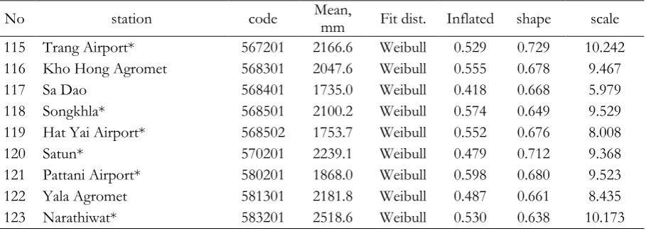
Thailand located in Southeast Asia and divided into 76 provinces covering an area of 513,120 square kilometers. Figure 1 shows Thailand, which is bordered by Myanmar and Laos in the north, Laos and Cambodia in the east, the Gulf of Thailand and Malaysia in the south, and the Andaman Sea and the southern extremity of Myanmar in the west. Generally, the weather is hot and humid because Thailand‘s location is between 5-20 degrees north latitude (the Tropical zone) [8, 9]. Thailand’s temperature normally ranges from 18 to 35 degrees Celsius and its annual rainfall ranges from 1,200 to 1,600 mm [10].

a warm air brought from the Indian Ocean, starts in May and ends in October, occurring rainfall in the country [12]. The northeast monsoon begins in October and finishes in February and brings cold and dry air from the Chinese mainland.

The inter-tropical convergence zone (ITCZ), equatorial trough or monsoon trough, which in the equatorial area is the convergence zone of two trade winds, northeasterly and southeasterly [13]. The Low atmospheric pressure area stills in the ITCZ with warm humid air rising and then cooling to produce rainfall. In May, this ITCZ arrives first in central Thailand and then moves in a northerly direction to China around June. The ITCZ moves south from China in July, dominating northern and northeastern Thailand in August with its second arrival, and later covers central and eastern Thailand in September, moving to the south Thailand in November.

Tropical cyclones and thunderstorm are the storm types in Thailand, causing a huge yearly rainfall. The tropical cyclones in Thailand come from the Pacific Ocean and the Indian Ocean [14, 15]. The South China Sea originates most of the tropical cyclones, tropical depression, tropical storm, and typhoon, which travel westward to Vietnam, Laos, Cambodia and Thailand. These cyclones cross northern and north-eastern Thailand in June to August and later move southward covering the central and eastern part from September to October, traveling across the south in November and December. In April, some cyclones originate in the Gulf of Thailand move through the east side of southern Thailand to the Andaman Sea before the southwest monsoon. In May, the beginning of rainy season, Myanmar and Thailand, the lower of the north, central and south, affected from the tropical cyclones originating in the Bay of Bengal. Thunderstorms, which are local storms, occur in summer from March to April, causing from convection and a confluence of a cold and warm moist air.

3.

Material and Methods

The aim of this study is to develop an asymmetric statistical distribution joined by the zero-inflated method to model daily rainfall intensity and find the best-fit distribution in Thailand. The method of determining the best model of daily rainfall organized as follows. The daily rainfall dataset was collected from observed rain gauges in Thailand that control the quality using the null value to remove a given year. The details are given in section a. An empirical cumulative distribution function (ECDF) represented by the referent dataset was analyzed by using the Kaplan-Meier method. We performed to improve the asymmetric statistical distribution equation with a zero-inflated algorithm to model the continuous data. This experiment used nine statistical distributions (Generalize Pareto (GP), Exponential (Exp), Beta, Gamma, Generalize extreme value (Gev), Extreme value (Ev), Log-normal, Weibull and Rayleigh distribution) that are usually used to model the rainfall data [4, 16, 17]. Details of mathematics equation are provided in section b. All distributions were evaluated by using the goodness of fit (GOF) and the residual ( ) and correlation ( ) coefficients were done by sorting the best fit distribution on each rain gauge.

3.1. Datasets

In this study, the daily rainfall data obtained from the Thai Meteorological Department Thailand. The data collected from 123 rain gauges across 73 provinces of Thailand, covering 43 years (1969-2011). Figure 2 shows the location of the collected rain gauges.

The mean record length is 37 years. The four rain gauges represented by highest annual averages are Klong Yai, Ranong, Takua Pa and Phriu Agromet over 3,000 mm/year. Because of the geographical location of these rain gauges, that located in orographic precipitation zone [18] and monsoon effect. In the middle of Thailand, covering 25 rain gauges in 3 parts, northern, northeastern and central part, have gotten the lowest annual rainfall. These rain gauges in the continental area of Southeast Asia, where the weather less affected from the monsoon [11].

3.2. Modeling Daily Rainfall Data

Daily observation rainfall data controlled a quality, using the null values. In this section, the continuous daily data analyzed and resulted in the cumulative distribution function (CDF). These data modeled, using nine statistical distributions.

We used the Kaplan-Meier method to estimate the ECDF represented by the observed data. The Kaplan-Meier (K-M) method, proposed by E. L. Kaplan and Paul Meier [19], is normally used for survival analysis in medical science, but is also applicable for time series data [20, 21] and rainfall data [22, 23]. This method summarized censored data and not assumed the value for constructing data distributions. The K-M method calculates the relative of data rank and statistical distribution based on right-censoring of the survival probability function.

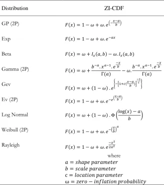
Count variables, which have zero values for underlying probability distribution of counts, modeled using the zero-Inflated method. The zero-inflated method, proposed by J. Mullahy [24] and Diane Lambert [25] has applied in economics, medical, public health and hydrology [26, 27]. The method divided into two sub-models, probability distributions of zero data and positive data. The general formula of the zero-inflated is.

( ) ( ) ( ) ₍₁₎

where is the count data; is the zero-inflation probability, and ( ) is the density of the count distribution.

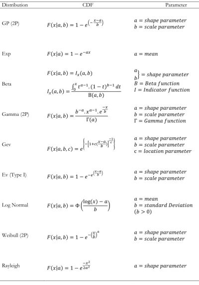
The nine Candidate statistical distributions were Generalize Pareto, Exponential, Beta, Gamma, Generalize extreme value, Extreme value, Log Normal, Weibull and Rayleigh distribution. Table 1 shows the nine candidate distributions represented in a CDF form. The Generalize Pareto (GP) is the ones of continuous statistical distribution. The GP distribution, usually applies to fit tails of other distribution, is specific by two parameters, shape and scale, in this study. The Exponential (Exp) distribution is done by one parameter as the mean that have been widely used for continuous distribution. The Exp distribution is used to simulate the time lapsed during the event. The Beta distribution is also the continuous distribution, which have been defined by the interval value between 0 to 1. This distribution has been done by two parameters for this study. The two parameters Gamma distribution has been used in this study that has a relationship with the Beta distribution. The Generalize extreme value (Gev) distribution is modified from the extreme value theory that has been developed from the Gumbel and Weibull distribution. The Gev distribution has three parameters, shape, scale and location, to use for this study. The Extreme value (Ev) have used in this study is type I (Gumbel). The Ev distribution has two parameters, shape and scale, to form in fitting the maximum number of sampling distribution. The Log Normal distribution is the continuous probability distribution that is represented by logarithm of normal distribution. In this study, the distribution have two parameter, mean and standard deviation of random variable that its standard deviation is greater than 0. The Weibull distribution is generally contained by three parameter, shape, scale and location, but this study have used the 2-pameter Weibull. The used Weibull have with the location parameter that value is 0. The Rayleigh distribution is specific in positive value of random variable, have one parameter as shape parameter.

We applied these nine distributions with the zero-inflection value into Eq. (1) that have shown in Table 2. The resulted distributions could be used to fit continuous daily rainfall data. In this study, these distributions had shape parameter ( ), scale parameter ( ), location parameter ( ), and zero probability value( ). The parameters were estimated by using maximum likelihood estimation method (MLE) that is occasionally used to optimize coefficient in statistical method [28]. The MLE is done by selecting a set of values of distribution parameters for underlying statistical distributions, where the selection parameter set maximizes the likelihood function [29–31]. The distribution parameters were searched to obtain results from the multi-dimension parameter sets [32].

Kolmogorov-Smirnov (K-S) test is a nonparametric test used to measure applicable continuous variable. The K-S test can be applied to evaluate the compatibility between empirical CDF (F(x)) and theoretical CDF (G(x)). The K-S statistic value is based on a maximum vertical difference of the both function [35, 36]. Comparing F(x) and G(x), the K-S statistic is

( ) ( ) (3)

Critical values of K-S test regarding the tested statistical distribution is rejected when the P-value of tested statistic is greater than the significance level of 5% that was mentioned in the previous paragraph. The P-value of the K-S test is

√ (4)

( ) ∑( )

(5)

where is a sample size of the CDF, is the integral probability distribution.

Anderson-Darling (A-D) test, proposed by T. W. Anderson and D. A. Daring [37], is normally used for testing a specified statistical distribution. The A-D test is modified to give more weight for the tail of the K-S test. This test statistic is defined as

∑( ) ( ) ( ( ))

(6)

The A-D test is screened out an unsuitable distribution based on the significance level of 5% to mention on above. P-value of the A-D test is used to reject when it is less than the critical values at 5%. The P-value of the A-D test is

( ) ( ( )) ₍₇₎

Chi-Square (C-S) test, developed by Pearson in 1900s is used to compare the statistical distribution and hypothesis test [38]. The C-S test is also a nonparametric statistical test, used like the K-S test to determine whether two or more classified data are independent or dependent [39]. This test is normally used to evaluate the fit model between simulated and observed value, statistic of the test is defined as

∑( )

(8)

where is the observed frequency for bin , is expected frequency for bin The expected frequency is estimated by

( ) ( ) (9)

where is the CDF of tested distribution, is the upper limit for , is the lower limit for , and is the sample size. A P-value of C-S test is depended on two variables, C-S statistic and degree of freedom ( ), and estimated by using the Gamma function. This test can reject the tested distribution based on the critical value at 5% also on above test. The P-value of the C-S test is

(10)

( ) ( ₎

∫

(11)

where is a sample size of the observation data.

CDF represented by ECDF and simulated CDF, was used to assess the best fit simulation distribution [16, 40]. The and coefficient are defined as

∑ (12)

∑ ( ) ∑ ( )

√∑ ( ) √∑ ( ) (13)

where is observed data, is estimated data and is a total number of sampling data.

The ranking method for finding the best fit distribution used a ranking number that represents among the nine distributions to create an order number between 1 and 9. The order number is marked on each distribution by using the and coefficient. To identify the order number, the distribution contain the lowest and the highest , is rank number 1, while the rank number 9 is the highest , and lowest . The best fit coefficient was calculated by an average of the ranking based on the , and coefficient. The best fit probability distribution was identified as the minimum of the best fit coefficient.

4.

Results and Discussion

The methodology mentioned above was applied to 123 rain gauges Thailand, covered 37 years of daily data for the continuous temporal data. According to a results, the cumulative distribution function (CDF) and the probability in the different distributions have shown in the first. Analysis of the results in the middle, a goodness-of-fit test, and a ranking test result were presented. Finally, the best-fit distribution of each rain gauge was shown.

On fitting distribution result, all rain gauges data were fitted by using the nine distributions resulted in CDF. The nine simulated CDFs were compared to ECDF by 95% confidence interval of the ECDF for evaluation. Kolmogorov-Smirnov (K-S), Anderson-Darling (A-D) and Chi-Square (C-S) test was used and analyzed on the nine distributions in each rain gauge to screen an incompatible distribution base on the level of significance. The incompatible distribution was identified by P-value on the significance level at 0.05. Table 3 shows the conformable distribution for selecting this compatible distribution based on the hypothesis test, when the two-thirds of 3 hypothesis tests were acceptable, the tested distribution was selected. On the other hand, unselected distribution was identified in the two-thirds of 3 hypothesis tests are rejected. The best-fit distribution was based on residual ( ) and correlation ( ) coefficient between simulation and observation CDF. For the best model, the minimum value of the and the maximum value of the were selected. Summary ranking could be calculated by the average of both coefficients, was used to identify the best-fit distribution. Weibull distribution among the eight distributions was the best model on the acid area. The 123 rain gauges have gotten the results with the processes as above.

The best probability distribution of all rain gauges (Fig. 3) was plotted by using its coordinate based on latitude and longitude. The rain gauge coordinate was used to distribute presented on the spatial map by using the Kriging algorithm [41]. The map was used to show the boundary of fitting distribution. The poorly fitted parameters of the spherical semi-variogram model on the spatial mapping were the nugget variance ( ) is 0.01, the partial sill ( ) is 0.04 and the range ( ) is 5.0 degree, are used to analyze. Weibull distribution conforms to 118 stations while 5 rain gauge stations fit to the Gamma distribution. Most of the stations, which are located in the continental area, fitted to the Weibull distribution. The 5 rain gauges accepted with the Gamma distribution are the highest annual rainfall zone that has been influenced by the monsoon and typhoon. Ranong station fitted to the Gamma that is located at the foot of the mountain and affected by the southwest monsoon and the Bengol Cyclone. Also, Phriu Agr and Khlong Yai same as the Ranong station where the location have influenced from the northeast monsoon and typhoon. While the both Nakhon Phanom station located far from the mountain are influenced by the typhoon to get the high annual rainfall and fitted to the Gamma distribution.

distribution [42]. Also, by the contrast, the fitted distribution on the previous study on the north-eastern part was presented by the Leakage distribution that was different to this study [3]. This study results showed the Weibull distribution that fitted to the rain gauge data on the north-eastern part. The results on the southern part was indirectly compared to neighbor area as Malesia that the fitted distribution of the neighbor country was Lognormal [5]. The fitted distribution of this study was the Weibull that contrasted to the previous study.

Generally, the modeling distribution results have gotten an effect from the difference of elevation and location of rain gauges, including monsoon and typhoon. Also, the results will be influenced by terrain and climate change.

5.

Concluding Remarks

Our goal was to consider compatible statistical distribution for daily rainfall data to simulate rainfall intensity. This research indicates that the continue data can be fitted by using probability distribution with a zero-inflated approach. The tested distributions are General Pareto, Exponential, Beta, Gamma, Generalize extreme value, Extreme value, Log-normal, Weibull, and Rayleigh distributions.

We found that a statistical distribution with zero-inflated on Weibull distribution was the most fitted distribution of daily rainfall intensity in Thailand with the goodness of fit score between observed and simulated value based on hypothesis test, maximum correlation ( ) and minimum residual ( ). In the second favorite distribution, the rain gauge stations were fitted by Gamma distribution, located in huge and orographic precipitation zone. In summary rainfall in Thailand, the rain gauge data are greatly influenced by their elevation, terrain and climate change to provide uncertainty on the rainfall distribution.

The scientific approach sufficiently established that the analytical methodology devised and test in this study may be utilized for the identification of the best fit statistical probability distribution of weather parameters. However, our statistical distributions can be used available to the scientific community through the hydrology modeling for use in the rainfall prediction application to water resources management and Meteorology research.

Acknowledgements

The study cannot be conducted without the data provided from various agencies, e.g., Royal Irrigation Department, Thai Meteorological Department and Land Development Department etc. Kochi University of Technology has been supported in part with Takagi laboratory.

References

[1] S. Dan‘azami, S. Shamsudin, and A. Aris, “Modeling of rainfall intensity using hourly data,” American Journal of Environmental Sciences, vol. 6, pp. 238-243, 2010.

[2] J. Suhaila and A. A. Jemain, “Fitting daily rainfall amount in Malaysia using the normal transform distribution,” Journal of Applied Sciences, vol. 7, pp. 1880-1886, 2007.

[3] H.N. Phien, A. Arbhabhirama, and A. Sunchindah, “Rainfall distribution in northeastern Thailand,”

Hydrological Sciences-Bulletin, vol. 25, pp. 167–182, 1980.

[4] L. S. Hanson and R. Vogel, “The probability distribution of daily rainfall in the United States,” in

World Environmental and Water Resources Congress 2008, Honolulu, Hawaii, USA, May 12-16, 2008, pp. 1-12.

[5] J. Suhaila,, K. Ching-Yee,, T. Fadhilah,, F. Hui-Mean,, “Introduction the mixed distribution in fitting rainfall data,” Open Journal of Modern hydrology, vol. 1, pp. 11-22, 2011.

[6] E. Ha and C. Yoo, “Use of mixed bivariate distributions for deriving inter-station correlation coefficients of rain rate,” Hydrological Processes, vol. 21, pp. 3078–3086, 2007.

[7] F. Famoye and K. P. Singh, “Zero-inflated generalized Poisson regression model with an application to domestic violence data,” Journal of Data Science, vol. 4, pp. 117–130, 2006.

[8] C. Thongkamsamut, “The building technological solution for hot humid climate modification in architecture,” International Journal of Renewable Energy, vol. 5, pp. 11–25, 2010.

[10] Climatological Centre, “Weather summary in Thailand report,” Meteorological Development Bureau Meteorological Department, BKK, Thailand, 2012.

[11] Y. Y. Loo, L. Billa, and A. Singh, “Effect of climate change on seasonal monsoon in Asia and its impact on the variability of monsoon rainfall in Southeast Asia,” International Journal of Renewable Energy, vol. 10, pp. 1–7, 2014.

[12] A. Limsakul, S. Limjirakan, and B. Suttamanuswong, “Asian summer monsoon and its associated rainfall variability in Thailand,” Environment Asia, vol. 3, pp. 79–89, 2010.

[13] T. Schneider, T. Bischoff, and G. H. Hang, “Migrations and dynamics of the intertropical convergence zone,” Nature, vol. 513, pp. 45–53, 2014.

[14] Climatological Centre, “Tropical cyclones in Thailand historical data 1951-2010 report,” Meteorological Development Bureau Meteorological Department, BKK, Thailand, 2011.

[15] P. A. Harr and J. C. L. Chan, “Monsoon impact tropical cyclone variability,” TMRP Report No. 70”, World Meteorological Organization, Hangzhou, China, 2005.

[16] M. A. Sharma and J. B. Singh, “Use of probability distribution in rainfall analysis,” New York Science Journal, vol. 3, pp. 40–49, 2010.

[17] S. Dan’azumi, S. Shamsudin, and A. A. Rahman, “Probability distribution of rainfall depth at hourly time-scale,” International Journal of Environment, Earth Science and Engineering, vol. 4, pp. 1–5, 2010.

[18] Q. Jiang, “Moist dynamics and orographic precipitation,” Tellus, vol. 55A, pp. 301–316, 2003.

[19] E. L. Kaplan and P. Meier, “Nonparametric estimation from incomplete observations,” Journal of the American Statistical Association, vol. 53, pp. 457–481, 1958.

[20] A. Picado, C. L. Lopes, R. Mendes, N. Vas, and J. M. Dias, “Storm surge impact in the hydrodynamics of tidal lagoon: the case of Ria de Aveiro,” Journal of Coastal Research, vol. 65, no. sp1, pp. 796–801, 2013.

[21] Z. Cai and G.G. Roussas, “Kaplan-Meier estimator under association,” Journal of Multivariate Analysis, vol. 67, pp. 318–348, 1998.

[22] A. Atencia, L. Mediero, M.C. Llasat, and L. Garrote, “Effect of radar rainfall time resolution on the predictive capability of a distributed hydrologic model,” Hydrology and Earth System Sciences, vol. 15, pp. 3809–3827, 2011.

[23] F. Oriani, J. Straubhaar, P. Renard, and G. Mariethoz, “Simulation of rainfall time series from different climatic regions using the direct sampling technique,” Hydrology and Earth System Sciences, vol. 18, pp. 3015–3031, 2014.

[24] J. Mullahy, “Specification and test of some modified count data models,” Journal of Econometrics, vol. 33, pp. 341–365, 1986.

[25] D. Lambert, “Zero-inflated poisson regression, with an application to defects in manufacturing,”

Technometrics, vol. 34, pp. 1–14, 1992.

[26] J. Ngatchou-Wandji and P. Chritophe, “On the zero-inflated count models with application to modelling annual trends in incidences of some occupational allergic diseases in France,” Journal of Data Science, vol. 9, pp. 639–659, 2011.

[27] J. Suhaila, K. Ching-Yee, F. Yusof, and F. Hui-Mean, “Effect of zero measurements in rainfall data,”

Journal Teknologi, vol. 63, pp. 35–39, 2013.

[28] I. J. Myung, “Tutorial on maximum likelihood estimation,” Journal of Mathematical Psychology, vol. 47, pp. 90–100, 2003.

[29] S. Geman and C. Hwang, “Nonparametric maximum likelihood estimation by the method of sieves,”

The Annals of Statistics, vol. 10, pp. 401–414, 1982.

[30] C. Uhler, “Geometry of maximum likelihood estimation in Gaussian graphical models,” The Annals of Statistics, vol. 40, pp. 238–261, 2012.

[31] K Huang, S. T. Guo, M. R. Shattuck, S. T. Chen, X. G. Qi, P. Zhang, and B. G. Li, “A maximum-likelihood estimation of pairwise relatedness for autopolyploid,” Heredity, vol. 114, pp. 133–142, 2015. [32] S. E. Fienberg and A. Rinaldo, “Maximum likelihood estimation in log-linear models,” The Annals of

Statistics, vol. 40, pp. 996–1023, 2012.

[33] A. Maydeu-Olivares, “Goodness-of-fit assessment of item response theory models,” Measurement: Interdisciplinary Research and Perspectives, vol. 11, pp. 71–101, 2013.

[34] R. D. Morey and E.J. Wagenmakers, “Simple relation between Bayesian order-restricted and point-null hypothesis tests,” Statistics and Probability Letters, vol. 92, pp. 121–124, 2014.

[36] A. Justel, D. Pefia, and R. Zamar, “A multivariate Kolmogorov-Smirnov test of goodness of fit,”

Statistics and Probability Letters, vol. 35, pp. 251–259, 1997.

[37] T. W. Anderson and D. A. Darling, “A test of goodness of fit,” Journal of the American Statistical Association, vol. 49, pp. 765–769, 1954.

[38] R. L. Plackett, “Karl Pearson and the chi-squared test,” International Statistical Review, vol. 51, pp. 59–72, 1983.

[39] S. D. Bolboaca, L. Jantschi, A. F. Sestras, R. E. Sestras, and D. C. Pamfil, “Pearson-Fisher chi-square statistic revisited,” Information, vol. 2, pp. 528–545, 2011.

[40] D. J. Prosser, J. Wu, E. C. Ellis, F. Gale, T. P. V. Boeckel, W. Wint, T. Robinson, X. Xiao, M. Gilbert, “Modelling the distribution of chickens, ducks, and geese in China,” Agriculture, Ecosystems and Environment, vol. 141, pp. 381–389, 2011.

[41] S. Ly, C. Charles, and A. Degre, “Geostatistical interporation of daily rainfall at catchment scale: the use of several variogram models in the Ourthe and Ambleve catchments, Belgium,” Hydrol. Earth Syst. Sci., vol. 15, pp. 2259-2274, 2011.

Appendix I: List of Tables

Table 1. Description of asymmetric statistical distribution functions.

Distribution CDF Parameter

GP (2P) _{( )} ( ₎

Exp ( )

Beta

( ) ( )

( ) ∫

_{( )}

( )

}

Gamma (2P) _{( )}

( )

Gev

( ) { [ (

)]

}

Ev (Type I) _{( )} ( )

Log Normal ( ) ( ( ) )

( )

Weibull (2P) _{( )} ( ₎

Table 2. Mixed distribution functions.

Distribution

ZI-CDF

GP (2P) _{( )} ( ₎

Exp ( )

Beta ( ) ( ) ( )

Gamma (2P) _{( )}

( )

( )

Gev

( ) ( ) { [ (

)]

}

Ev (2P) _{( )} ( )

Log Normal ( ) ( ) ( ( ) )

Weibull (2P) _{( )} ( ₎

Rayleigh _{( )}

where

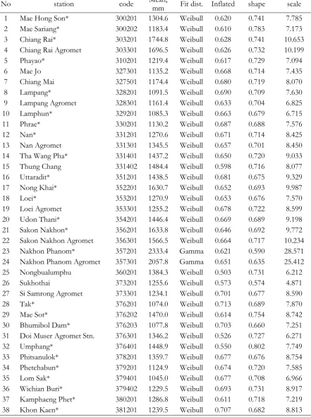
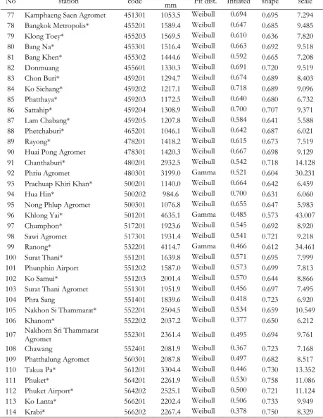
Table 3. The fit parameter of best fit distribution in each rain gauge.

No station code Mean, _mm Fit dist. Inflated shape scale 1 Mae Hong Son* 300201 1304.6 Weibull 0.620 0.741 7.785 2 Mae Sariang* 300202 1183.4 Weibull 0.610 0.783 7.173 3 Chiang Rai* 303201 1744.8 Weibull 0.628 0.741 10.653 4 Chiang Rai Agromet 303301 1696.5 Weibull 0.626 0.732 10.199 5 Phayao* 310201 1219.4 Weibull 0.617 0.729 7.094 6 Mae Jo 327301 1135.2 Weibull 0.668 0.714 7.435 7 Chiang Mai 327501 1174.4 Weibull 0.680 0.719 8.070 8 Lampang* 328201 1091.5 Weibull 0.690 0.709 7.630 9 Lampang Agromet 328301 1161.4 Weibull 0.633 0.704 6.825 10 Lamphun* 329201 1085.3 Weibull 0.663 0.679 6.715 11 Phrae* 330201 1130.2 Weibull 0.687 0.688 7.576

12 Nan* 331201 1270.6 Weibull 0.671 0.714 8.425

13 Nan Agromet 331301 1345.5 Weibull 0.657 0.701 8.450 14 Tha Wang Pha* 331401 1437.2 Weibull 0.650 0.720 9.033 15 Thung Chang 331402 1484.4 Weibull 0.598 0.716 8.077 16 Uttaradit* 351201 1438.5 Weibull 0.681 0.675 9.329 17 Nong Khai* 352201 1630.7 Weibull 0.652 0.693 9.987 18 Loei* 353201 1270.9 Weibull 0.653 0.676 7.570 19 Loei Agromet 353301 1255.2 Weibull 0.678 0.722 8.599 20 Udon Thani* 354201 1446.4 Weibull 0.669 0.689 9.198 21 Sakon Nakhon* 356201 1633.8 Weibull 0.646 0.692 9.772 22 Sakon Nakhon Agromet 356301 1566.5 Weibull 0.664 0.717 10.234 23 Nakhon Phanom* 357201 2333.4 Gamma 0.621 0.590 28.571 24 Nakhon Phanom Agromet 357301 2057.8 Gamma 0.651 0.635 25.412 25 Nongbualumphu 360201 1384.3 Weibull 0.503 0.731 6.212 26 Sukhothai 373201 1255.6 Weibull 0.573 0.574 4.871 27 Si Samrong Agromet 373301 1234.1 Weibull 0.701 0.677 8.590

28 Tak* 376201 1074.0 Weibull 0.713 0.689 7.870

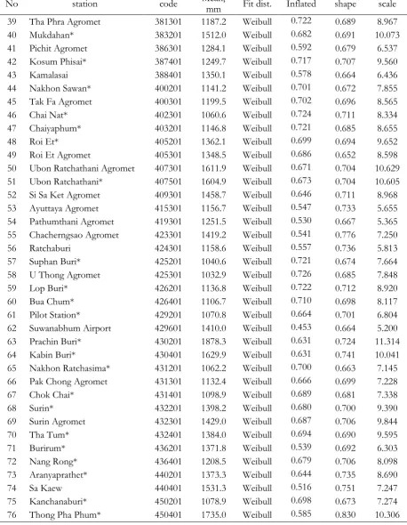
Table 3. The fit parameter of best fit distribution in each rain gauge (continues).

No station code Mean, _mm Fit dist. Inflated shape scale 39 Tha Phra Agromet 381301 1187.2 Weibull 0.722 0.689 8.967 40 Mukdahan* 383201 1512.0 Weibull 0.682 0.691 10.073 41 Pichit Agromet 386301 1284.1 Weibull 0.592 0.679 6.537 42 Kosum Phisai* 387401 1249.7 Weibull 0.717 0.707 9.560 43 Kamalasai 388401 1350.1 Weibull 0.578 0.664 6.436 44 Nakhon Sawan* 400201 1141.2 Weibull 0.701 0.672 7.855 45 Tak Fa Agromet 400301 1199.5 Weibull 0.702 0.696 8.565 46 Chai Nat* 402301 1060.6 Weibull 0.724 0.711 8.334 47 Chaiyaphum* 403201 1146.8 Weibull 0.721 0.685 8.655 48 Roi Et* 405201 1362.1 Weibull 0.699 0.694 9.652 49 Roi Et Agromet 405301 1348.5 Weibull 0.686 0.652 8.598 50 Ubon Ratchathani Agromet 407301 1611.9 Weibull 0.671 0.704 10.629 51 Ubon Ratchathani* 407501 1604.9 Weibull 0.673 0.704 10.605 52 Si Sa Ket Agromet 409301 1458.7 Weibull 0.646 0.711 8.968 53 Ayuttaya Agromet 415301 1156.7 Weibull 0.547 0.733 5.655 54 Pathumthani Agromet 419301 1251.5 Weibull 0.530 0.667 5.365 55 Chacherngsao Agromet 423301 1419.2 Weibull 0.541 0.776 7.250 56 Ratchaburi 424301 1158.6 Weibull 0.557 0.736 5.813 57 Suphan Buri* 425201 1040.6 Weibull 0.721 0.674 7.664 58 U Thong Agromet 425301 1032.9 Weibull 0.726 0.685 7.848 59 Lop Buri* 426201 1136.8 Weibull 0.722 0.712 8.920 60 Bua Chum* 426401 1106.7 Weibull 0.710 0.698 8.117 61 Pilot Station* 429201 1070.8 Weibull 0.664 0.701 6.804 62 Suwanabhum Airport 429601 1410.0 Weibull 0.453 0.664 5.200 63 Prachin Buri* 430201 1878.3 Weibull 0.631 0.724 11.314 64 Kabin Buri* 430401 1629.9 Weibull 0.631 0.741 10.041 65 Nakhon Ratchasima* 431201 1062.2 Weibull 0.700 0.663 7.145 66 Pak Chong Agromet 431301 1132.4 Weibull 0.666 0.699 7.228 67 Chok Chai* 431401 1098.9 Weibull 0.689 0.681 7.338

68 Surin* 432201 1398.2 Weibull 0.680 0.700 9.390

Table 3. The fit parameter of best fit distribution in each rain gauge (continues).

No station code Mean, _mm Fit dist. Inflated shape scale 77 Kamphaeng Saen Agromet 451301 1053.5 Weibull 0.694 0.695 7.294 78 Bangkok Metropolis* 455201 1589.4 Weibull 0.647 0.685 9.485 79 Klong Toey* 455203 1569.5 Weibull 0.610 0.636 7.820 80 Bang Na* 455301 1516.4 Weibull 0.663 0.692 9.518 81 Bang Khen* 455302 1444.6 Weibull 0.592 0.665 7.208 82 Donmuang 455601 1330.3 Weibull 0.691 0.720 9.519 83 Chon Buri* 459201 1294.7 Weibull 0.674 0.689 8.403 84 Ko Sichang* 459202 1217.1 Weibull 0.718 0.689 9.096 85 Phatthaya* 459203 1172.5 Weibull 0.640 0.680 6.732 86 Sattahip* 459204 1308.9 Weibull 0.700 0.707 9.371 87 Lam Chabang* 459205 1207.8 Weibull 0.584 0.641 5.588 88 Phetchaburi* 465201 1046.1 Weibull 0.642 0.687 6.021 89 Rayong* 478201 1418.2 Weibull 0.615 0.673 7.519 90 Huai Pong Agromet 478301 1420.3 Weibull 0.667 0.698 9.129 91 Chanthaburi* 480201 2932.5 Weibull 0.542 0.718 14.128 92 Phriu Agromet 480301 3199.0 Gamma 0.521 0.604 30.231 93 Prachuap Khiri Khan* 500201 1140.0 Weibull 0.664 0.642 6.459 94 Hua Hin* 500202 984.6 Weibull 0.700 0.631 6.060 95 Nong Phlup Agromet 500301 1076.8 Weibull 0.655 0.647 5.983 96 Khlong Yai* 501201 4635.1 Gamma 0.485 0.573 43.007 97 Chumphon* 517201 1923.6 Weibull 0.545 0.692 8.920 98 Sawi Agromet 517301 1931.4 Weibull 0.541 0.721 9.218

99 Ranong* 532201 4114.7 Gamma 0.466 0.612 34.461

Table 3. The fit parameter of best fit distribution in each rain gauge (continues).

Appendix II: List of Figures