Distributed Coordination and Optimisation of Network-Aware Electricity Prosumers

(1)

Distributed Coordination and Optimisation of

Network-Aware Electricity Prosumers

Paul Scott

November 2016

A thesis submitted for the degree of

Doctor of Philosophy of

The Australian National University

(2)

(3)

Declaration

Except where otherwise stated, this thesis is my own original work.

Paul Scott November 2016

(4)

(5)

Acknowledgements

Firstly, I would like to thank to Sylvie Thi´ebaux for being a fantastic super-visor and mentor. Your advice and help has been invaluable and I greatly appreciate the time you invested. Thank you also to my supervisor Pascal Van Hentenryck and advisor Menkes van den Briel for your technical help, ideas and advice.

Thanks to Hassan Hijazi, Carleton Coffrin and Archie Chapman for shar-ing your expert technical knowledge and for the valuable discussions. To my fellow students Karsten, Josh, Jan, Fazlul, Hadi, Terrence and Boon Ping, I had a great time working with you and sharing in the experiences of PhD life.

Finally, I would like to acknowledge my family and friends, with a special thanks to Megan for all her encouragement, understanding and support.

(6)

(7)

Abstract

Electricity networks are undergoing a transformation brought on by new technologies, market pressures and environmental concerns. This includes a shift from large centralised generators to small-scale distributed generat-ors. The dramatic cost reductions in rooftop solar PV and battery storage means that prosumers (houses and other entities that can both produce and consume electricity) will have a large role to play in future networks.

How can networks be managed going forward so that they run as effi-ciently as possible in this new prosumer paradigm? Our vision is to treat prosumers as active participants by developing a mechanism that incentiv-ises them to help balance power and support the network. The whole process is automated to produce a near-optimal outcome and to reduce the need for human involvement.

The first step is to design an autonomous energy management system (EMS) that can optimise the local costs of each prosumer in response to network electricity prices. In particular, we investigate different optimisation strategies for an EMS in an uncertain household environment. We find that the uncertainty associated with weather, network pricing and occupant behaviour can be effectively handled using online optimisation techniques using a forward receding horizon.

The next step is to coordinate the actions of many EMSs spread out across the network, in order to minimise the overall cost of supplying elec-tricity. We propose a distributed algorithm that can efficiently coordinate a network with thousands of prosumers without violating their privacy. We experiment with a range of power flow models of varying degrees of ac-curacy in order to test their convergence rate, computational burden and solution quality on a suburb-sized microgrid. We find that the higher accur-acy model, although non-convex, converges in a timely manner and produces near-optimal solutions. We also develop simple but effective techniques for dealing with residential shiftable loads which require discrete decisions.

The final part of the problem we explore is prosumer manipulation of the coordination mechanism. The receding horizon nature of our algorithm is great for managing uncertainty, but it opens up unique opportunities for prosumers to manipulate the actions of others. We formalise this form of receding horizon manipulation and investigate the benefits manipulative

(8)

agents can obtain. We find that indeed strategic agents can harm the system, but only if they are large enough and have information about the behaviour of other agents. For the rare cases where this is possible, we develop simple privacy-preserving identifiers that monitor agents and distinguish manipu-lation from uncertainty.

(9)

Introduction

Electricity networks are undergoing a huge transformation due to the emer-gence of new technologies, market pressures and environmental concerns. The most significant trend is the transition from large centralised to small distributed forms of generation. The adoption of rooftop solar is shifting the ownership and control of generation away from large companies and into the hands of consumers. Such prosumers (houses and other entities that can both produce and consume electricity) have the opportunity to meet significant portions of their own energy needs and to sell excess power. Distributed generation both positively and negatively affects electricity networks. It can reduce losses and allow for leaner, cheaper network designs; however, the weather dependent nature of distributed generation like solar photovoltaics (PV) means that supply does not always align with demand. In addition to this, uncontrolled or uncoordinated distributed generation can create voltage, peak power flow and ramping problems for networks.

Solar PV is already causing problems in some networks, and it will only get worse with time. For example, in some areas of the Australian network, the amount of rooftop PV has reached the point where utilities have to limit or reject new proposals if the impacts are assessed to be adverse [AEMO, 2012, CAT Projects and ARENA, 2015]. The only other option utilities currently have, network augmentation, is cost-prohibitive.

Other types of distributed energy technologies (DETs), including battery storage, electric vehicles (EVs) and smart appliances, pose similar oppor-tunities but also similar risks to the network as PV [Ramchurn et al., 2012, Kok et al., 2009].

This thesis explores a new way forward for prosumers and utilities, where they work together to operate the network as efficiently and safely as pos-sible. It addresses the question:

How can DETs be operated so that the benefits to prosumers are maximised whilst also supporting the network?

(14)

In answering this question, we will enable networks to embrace higher levels of DETs, most importantly rooftop PV and EVs. This will allow net-works to operate more efficiently, with lower emissions and at lower cost. Prosumers will benefit through lower network costs, greater flexibility, re-wards for actively supporting the network, and better utilisation of their DET assets.

We identify three parts that are necessary for a technical solution to the above problem, which form the motivation for the work in this thesis:

1. having autonomous controllers for DETs that can minimise prosumer energy costs in an uncertain environment;

2. coordinating the actions of multiple prosumer controllers to reduce system-wide costs and satisfy network constraints; and

3. aligning the motivations of self-interested prosumers with what is fa-vourable for the wider network.

When combined, these parts deliver a technical solution for the distrib-uted coordination and optimisation of network-aware electricity prosumers.

Home Energy Management

The first part of this thesis recognises the need to automatically control DETs so that the amount of human interaction is minimised. Prosumers do not want to invest time in manually controlling their devices, and even if they did, they would likely make poor decisions. Instead, what we propose is an automated energy management system (EMS) that acts on behalf of the prosumer to optimise their energy needs and costs, in a way that is transparent and does not encroach on their freedom.

We focus on the development of an EMS for household prosumers (see figure 1.1), although the same the techniques could be applied to commercial, industrial or other types of prosumers. Houses are the most numerous (and interesting) type of network participant, accounting for around 25% of the total electricity consumption in countries like Australia [Vivid Economics, 2013].

The EMS communicates with devices present in the house and with the network. The house occupants provide simple, high-level preferences and constraints to the EMS, which then schedules the operation of the devices in a way that minimises energy costs.

(15)

3

[image:15.595.130.419.125.345.2]

26

Figure 1.1: An EMS controls household DETs including batteries, EVs, space heating/cooling and smart appliances.

beneficial to align consumption within the house with the solar PV output, which is not possible without a good prediction of solar production.

We design an EMS that can make sensible decisions in the face of uncer-tainty, using ideas from model predictive control (MPC), receding horizon control [Morari and Lee, 1999] and online stochastic optimisation [Van Hen-tenryck and Bent, 2006]. The EMS schedules the operation of devices over a forward horizon, using stochastic models for the uncertainty. This is cru-cial because the operation of state-based household devices (e.g., battery charge) needs to be planned out over multiple time steps. The EMS also operates online, updating its stochastic models and schedule as it progresses, enabling it to recover from poor earlier decisions and to take advantage of new opportunities.

We develop models for the devices and stochastic models for the uncer-tain aspects of the problem. Two different online algorithms are developed that use mixed-integer programming, and are compared to more reactive forms of control in an uncertain home environment—something that is miss-ing from the existmiss-ing literature.

(16)

computational burden.

These results show that, in practice, the uncertainty present in houses can be managed with computationally efficient methods and that the case for automating energy management is strong. The EMS can make local control decisions on behalf of occupants, providing the building blocks for the wide-scale control of DETs.

Network-Aware Coordination

The next step is to expand beyond a single prosumer by considering how multiple EMSs impact the network. When prosumers are left to optimise their own costs in an uncoordinated manner, the combination of their de-cisions can create undesirable new peaks in supply and demand [Ramchurn et al., 2011]. This effect, known as herding, has the potential to cause price volatility, and large voltage, ramping and line limit problems [Farhoodnea et al., 2013, de Hoog et al., 2013, Cain et al., 2010, Roozbehani et al., 2012]. To illustrate this problem, consider a network where prosumers own EVs and are subject to peak/off-peak pricing. If the off-peak period starts at 10 pm, then many of the EVs will be scheduled to begin charging at 10 pm, which could create a large spike in demand. On the other hand, spikes in supply can be produced in sunny conditions by PV systems when the overall demand for electricity is low. We cannot consider agents in isolation if we want to ensure the safe operation of the network and the efficient utilisation of available assets.

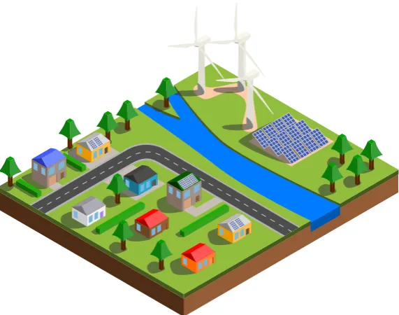
This motivates the next step where we take a network of prosumers with EMSs and look at the larger problem of jointly optimising prosumer and network costs. We take a network-aware approach, which means that we explicitly model the flow of power on the network to correctly account for the network’s behaviour and limitations. Conventional networks already perform a similar task for large generating units, minimising dispatch costs whilst obeying transmission network constraints. When this is extended to allow prosumer participation, a significantly different approach is required. Firstly, the scale of the problem is much larger than the conventional dispatch problem. Instead of coordinating a few hundred generating units, now many thousands or even millions of participants need to be considered (see figure 1.2). Secondly, the distributed nature of the problem means that localised distribution network constraints become significant, where before they could be ignored. Finally, prosumers have a more diverse range of behaviours and sensitivities which need to be considered.

(17)

[image:17.595.131.417.124.349.2]

5

Figure 1.2: A small sample of the many thousands of connected prosumers and distributed generators that need to be coordinated to balance the network.

(ADMM) [Boyd et al., 2011], works by locally exchanging price and power consumption/production information between prosumer EMSs and neigh-bouring network components. The algorithm negotiates a set of dynamic nodal prices and power allocations for the network and its participants. The prices accurately represent the marginal cost of supplying power to that part of the network, and are used to charge/pay prosumers for their actions. As power allocations for each prosumer are negotiated ahead of time, it pre-vents the herding effect exhibited by other pricing methods that have no two-way negotiation.

The handling of network and prosumer non-convexity in distributed al-gorithms is a significant unresolved problem that we tackle. Tractable dis-tributed algorithms do not provide any guarantees of optimality when the underlying problem is non-convex. Unfortunately, the equations that model the physical flow of power on the network are non-convex, and the opera-tion of certain household devices requires discrete decisions to be made. We investigate how such non-convexities can be managed in a tractable manner without sacrificing the quality of solutions.

(18)

The end result is to show that a distributed approach to optimising and coordinating EMSs is not only possible, but highly effective.

Receding Horizon Manipulation

The final contribution is to ensure that the incentives offered to prosumers are aligned with the social objective of minimising the total system costs. Our distributed algorithm minimises the social objective, but only if agents act truthfully. By lying about their costs and constraints, prosumers can reduce their own costs, at the detriment of others prosumers and the so-cial objective. We want to reduce the ability of agents to perform such

manipulation and its impact on the system.

Existing electricity markets are already vulnerable to manipulation, with generating units adjusting their bidding strategies to maximise their ad-vantage. Beyond this, the receding horizon nature of our algorithm creates unique opportunities for manipulation. The receding horizon is great for dealing with uncertainty, but the added flexibility also allows more oppor-tunity for agents to manipulate others.

[image:18.595.161.482.498.566.2]

To illustrate this form of manipulation, take two neighbours, Alice and Bob, who both want to charge their EVs at 9 pm (see figure 1.3). The social solution is for them to both charge at 9 pm. Alice realises that if it were just her charging at 9 pm then the price will be lower. She artificially and temporarily raises the price at 9 pm by claiming to require more power than she actually needs. To avoid the price Bob charges at 8 pm. After Bob has finished charging, Alice can start telling the truth, allowing the price at 9 pm to reduce to a value lower than in the social solution.

Figure 1.3: Two homes competiting to charge their electric vehicles.

It is difficult to correctly identify that Alice actually manipulated Bob, as we do not have access to her private information, and she could pretend that she was uncertain about her consumption requirements. There is a conflict between allowing agents to recover from uncertainty while also preventing manipulation.

We investigate receding horizon manipulation in detail. We develop a

(19)

7

harms the system. We then develop non-invasive techniques which can be used to detect this form of manipulation. If successfully identified, agents can be fined or be subject to further auditing processes.

We find that it is possible for large agents or a large coalition of agents to gain an advantage and harm the overall social objective. We manage to successfully apply our identifiers to the actions of these agents, and distin-guish their actions as being manipulative as opposed to just being honestly uncertain. It does not completely eliminate manipulation, but it acts as a strong deterrent, and makes it more difficult to calculate beneficial manip-ulative strategies. Our framework allows new identifiers to be added over time if agents develop new strategies.

Summary

To summarise, the key research question we tackle is how to operate distrib-uted energy technologies in a way that maximises the benefits to prosumers whilst also supporting the network. We address this question in three parts that come together to form a complete solution: the development of autonomous home EMSs that can operate in an uncertain environment; the coordination of these EMSs across the network to reduce system-wide costs while satisfying network constraints; and the development of identifiers that deter strategic agents from manipulating the system.

We contribute to knowledge in each of these areas:

• We show how online stochastic optimisation based on a receding hori-zon can be used to efficiently control devices within a house, and that it produces solutions that compare favourably with a perfect inform-ation case. It was found to have significant advantages over reactive forms of control.

• We establish the suitability of different power flow models in a distrib-uted optimisation setting and, how the non-convex power flow equa-tions can be used directly to produce near-optimal results. Similarly, we show how discrete shiftable house loads in practice can be included in the distributed algorithm, and still achieve near-optimal results.

• We determine in the worst case how much strategic agents have to gain and how much they can harm the performance of the system. We formalise receding horizon manipulation in this power exchange setting, and develop and demonstrate identifiers that can distinguish strategic agents from uncertain agents.

(20)

new flexible and efficient solutions. Our work develops a key component of the solution, by enabling prosumers to participate actively in the balancing and management of the network.

Thesis Outline

This thesis is structured as follows:

Chapter 2 provides a non-technical introduction to power systems, look-ing at topics such as energy markets, generation and power transmis-sion/distribution. It also dedicates sections to describing the different types of DETs and the different approaches that have been used to incentivise and coordinate them.

Chapter 3 introduces the residential energy management problem and de-velops online stochastic optimisation techniques for scheduling DETs in the presence of uncertainty. These algorithms are compared with reactive controllers and a clairvoyant controller on a household test case.

Chapter 4 extends this to the wider problem of how to coordinate EMSs over the network. A distributed algorithm is developed to perform the coordination and is experimented with on a test microgrid for different power flow models and methods for handling discrete decisions.

Chapter 5 investigates the potential for manipulation of the receding ho-rizon mechanism. It formalises receding hoho-rizon manipulation, exper-iments with a greedy strategic agent and develops identifiers to detect this type of manipulation.

(21)

Chapter 2

Background

This chapter provides background material that sets the context and motiv-ation for our problem. First we introduce power systems and what changes distributed energy technologies (DETs) are causing. Then we introduce the different types of DETs and the types of methods that have been proposed for controlling/coordinating them. In later chapters we develop our dis-tributed algorithm with these DETs in mind, and perform more detailed comparisons to existing approaches.

Where relevant, later chapters include more topic-specific background material. Chapter 3 has a section on stochastic programming, chapter 4 contains sections on power flows and distributed optimisation, and chapter 5 has a section on mechanism design.

2.1 Power Systems

Electric power systems (also known as grids or networks) have been used for over a century to supply energy to our industries and homes, playing a cent-ral role in enabling the technological and quality-of-life improvements over this time. This section provides an overview of conventional power systems and discusses the pressures they are experiencing from new technologies and environmental concerns.

To help explain power systems, we refer to the National Electricity Mar-ket (NEM) in Australia. The NEM network spans the east coast of Australia, supplying some 19 million residents [AEMO, 2015a]. Many parallels can be drawn between the NEM and other deregulated electricity markets such as those in the USA.

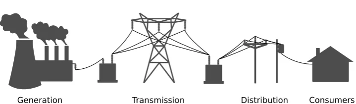
Power systems consist of three main components: generators, consumers and the network of conductors that transport power between the two. The network is further divided into the transmission and distribution networks (see figure 2.1). Conventional power systems are operated by central au-thorities which manage the dispatch of generation and control of network

(22)

components.

[image:22.595.142.502.144.249.2]

Generation Transmission Distribution Consumers

Figure 2.1: The main components of a power system.

2.1.1 Markets

In deregulated power systems, markets play a key role in facilitating the sup-ply of electricity and coordinating operational decisions. These centralised markets focus on coordinating the dispatch of large generation units and managing the transmission network. In chapter 4 we construct a market of our own, but one that coordinates prosumers and other network participants in a decentralised way on the distribution network.

Wholesale energy supply markets ensure that there is always enough bulk supply dispatched to meet forecast demand. Frequency regulation markets recruit generators to balance any wholesale market supply and demand pre-diction errors in real time.

The NEM is made up of one wholesale energy supply market (the spot market) and 8 frequency control markets. Generators bid into the market the amount of power they can supply for a particular price. The NEM dispatch engine clears the market every 5 minutes by selecting the lowest cost bids to match the forecast demand. The spot price is a 30 minute average of these dispatch prices, and it is the price at which all dispatched generators get paid.

Retailers buy electricity at the spot market price and onsell it to con-sumers. The retail tariffs offered to consumers vary between regions and depend on the type of customer (e.g., residential, commercial or industrial). Residential tariffs are typically either constant or time-of-use (TOU) where they change for different times of the day. Section 2.3.3 will discuss other more dynamic forms of pricing.

(23)

2.1. POWER SYSTEMS 11

Wholesale

Retail

Transmission

[image:23.595.167.384.127.270.2]

Distribution

Green Schemes

Figure 2.2: Breakdown of NEM residential electricity bill costs in 2014 [AER, 2014].

2.1.2 Generation

Generators get their energy from either renewable (hydro, wind and solar) or non-renewable (coal, gas, oil and nuclear) sources. In most countries the majority of electricity still comes from non-renewable sources. Table 2.1 shows how coal supplies around 75% of the NEM electricity.

Table 2.1: NEM capacity and production by generator type for 2014/15 financial year [AER, 2015]. Only includes registered generators (no rooftop PV).

Type Capacity (%) Production (%)

Black Coal 39.2 50.8 Brown Coal 14.3 25.7

Gas 20.1 11.6

Hydro 16.5 6.6

Wind 6.6 4.8

Other 3.2 0.5

Generators are dispatched so that supply always matches demand on the network. The network itself cannot store electricity, so any mismatch will cause fluctuations in frequency and voltage, which can ultimately damage equipment or trigger a blackout. This dispatch problem is becoming more challenging as networks transition away from large centralised forms of gen-eration to small distributed generators, which is our primary motivation for using DETs to help balance supply and demand.

(24)

as wind and solar, have effectively zero marginal running costs, but their availability is weather dependent.

As such, coal power stations provide a steady base-load supply and gas turbines are typically peaking plants that get dispatched during peak load or high ramping rate conditions. The near-zero running costs of renew-ables means that they get dispatched whenever they are available. These behaviours are observed in table 2.1 when the normalised amount of energy each generator typecould provide (capacity) is compared to the normalised amount of energy itactuallyproduced (production). For example, although gas has 20.1% of the total capacity, it is only used to supply 11.6% of the actual load.

In most networks the vast majority of electricity comes from a relatively small number of very large power plants. For example, the NEM has less than 400 registered generating units, with the 100 largest having around 80% of the total network capacity [AEMO, 2015b] (see figure 2.3). These 100 generating units are from around 40 individual power plants, which is a tiny number when compared to the near 9 million metered consumers that the NEM serves.

Figure 2.3: The Yallourn W brown coal power station alone supplies around 8% of the NEM’s electricity (“Yallourn Power Station” by CSIRO, CC BY 3.0).

Large generators often have to be situated far from where the energy is needed for public safety reasons and/or the need to be collocated with a geographical feature (e.g., a coal mine, water source or hydro dam). The transmission network serves the role of transporting high volumes of electri-city from the generators to where it is needed.

(25)

2.1. POWER SYSTEMS 13

costs have outdone expectations, with recent studies estimating that utility-scale PV is already competitive with conventional generation in countries such as the US [Lazard, 2015].

These cost comparisons are for generators in the wholesale market, but renewables like PV are able to compete in the retail market by being installed in homes behind the meter. As shown previously in figure 2.2, the wholesale prices contribute only around 20% of the total retail costs in the NEM. This makes PV much more competitive installed in homes than it would otherwise be in the wholesale market, primarily because it bypasses the expensive network altogether by supplying power directly where it is needed. Such behind-the-meter PV makes up the majority of the installed PV, which was around 2.5% of the total electricity consumed in the NEM in 2014 [Johnston et al., 2015].

2.1.3 Transmission

Transmission networks provide high volume transport of electricity between generators and load centres (e.g., cities). Figure 2.4 shows the transmission network for the NEM which spans the whole Australian east coast con-necting generators, cities and regional towns. This thesis focuses on what happens further downstream on the distribution network, as this is where DETs will have most impact; however, the same techniques can be applied to manage the transmission network.

Structurally, transmission networks are meshed (contain cycles) and are often designed and operated to beN−1 reliable, which requires that the fail-ure of any one line, generator or network component will not bring the whole system down. Most networks are 3-phase alternating current (AC) with a small number of high voltage direct current (DC) links where economically viable.

Transmission networks operate at high voltages (typically in range 100kV to 500kV in the NEM) and are much more heavily instrumented, mon-itored and managed than distribution networks because of their more critical nature. The operators of transmission networks are concerned with issues of voltage regulation, managing congestion and stability.

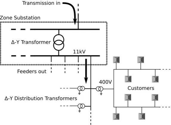
2.1.4 Distribution

(26)

[image:26.595.197.431.118.428.2]

Figure 2.4: NEM transmission lines and generators (image adapted with permission from AER [2014]).

through built-up areas. These medium voltage lines, called feeders, connect to distribution transformers close to consumers. Distribution transformers bring the voltage down to the final voltage for consumption (400V three phase or 230V single phase for residential customers in the NEM).

Meters are used to record how much power enters the distribution net-work from the transmission netnet-work and how much leaves the netnet-work at the point of customer connection. AC power is split up into two components,

real power which does actual work, andreactive power which oscillates back and forth between active electrical components (see appendix A for more details). Residential customers are typically only billed for real power con-sumption, while larger customers are also billed for their peak consumption of real and reactive power.

(27)

under-2.1. POWER SYSTEMS 15

11kV Transmission in

Δ-Y Transformer Zone Substation

Feeders out

Δ-Y Distribution Transformers

[image:27.595.130.417.124.334.2]

Customers 400V

Figure 2.5: The layout of a distribution network. Distribution transformers have 4 conductor outputs, one for each phase and a neutral. Customers connect to either a single phase or to three phases.

utilised for the rest of the time. The techniques we develop in this thesis for the intelligent control of DETs can reduce these peaks and hence greatly reduce distribution network costs.

2.1.5 Microgrids

Microgrids are an emerging technology which hold particular promise in developing nations. Microgrids are small-scale networks (ranging in size from a small community all the way up to an entire city) that can disconnect from and operate independently of the rest of the network [Glover et al., 2011]. Microgrids provide a number of advantages including better resilience to faults on the network, and more organic and gradual electrification of remote or rural areas.

Like more conventional centralised networks, microgrids need to ensure that power is balanced, frequency is maintained and the network is safely operated. These events take place on a smaller scale, which means that there is more uncertainty and less room for error. In chapter 4 we test our distributed algorithm on a community-scale microgrid.

2.1.6 Consumption

(28)

2013]. In this thesis we focus on residential customers; however, the same techniques we develop could be applied to participants in the other sectors. This focus is because residential customers:

• in aggregate have a large share of the overall consumption;

• are the most numerous;

• are the early adopters of many DETs such as PV, EVs and battery storage; and

• are widely dispersed throughout the network.

Figure 2.6 shows the consumption pattern for one house over a single day. The load profile has large peaks caused by the operation of different appliances. The power profile tends to smooth out as the loads of many houses are combined, but there are still events which are correlated between homes (e.g., working schedules, air conditioner usage and PV production). The aggregate profile tends to exhibit peaks in the morning and evening as residents leave for and return from work. By scheduling the operation of DETs (e.g., a smart dishwasher), the load profile of both a single house and the aggregate of many houses can be shaped. Chapter 3 investigates in detail how to optimise the operation of DETs within a single house (prosumer).

0

6

12

18

24 Time (hrs)

0

500 1000

1500

2000

Power (W)

[image:28.595.158.482.446.684.2]

Outlets

Lighting

Microwave

Fridge

Dishwasher

(29)

2.2. DISTRIBUTED ENERGY TECHNOLOGIES 17

2.2 Distributed Energy Technologies

DETs are any generators or controllable loads that are of a small enough scale that they can be connected directly to the distribution system or be-hind the meters of customers. The rapid development of such technologies is challenging the conventional notion of how networks are designed and operated.

As discussed previously, DETs are shifting generation away from large centralised power stations and are enabling individuals or communities to have more control over their own energy requirements. For example, DETs enable the formation of community owned microgrids, which can either op-erate stand-alone or trade energy with the wider network.

This thesis will often refer to consumers (houses or any agents) that have control and ownership over a set of DETs asprosumers. This captures the idea that they can both consume and produce energy, and that they are more involved in managing their own energy requirements.

The following sections describe some of the DETs that are available to houses, and which we will be working with in later chapters. We discuss their behaviour and what they can be used for. They range from batteries that can be charged or discharged on command, to less controllable solar PV generators.

2.2.1 Generators

Distributed generation ranges from the renewable-sourced solar PV and wind generators which have limited controllability to the dispatchable fuel-based micro gas turbine, diesel and fuel-cell generators. Solar PV is safe, low maintenance, unobtrusive and affordable, making it ideal for residen-tial use. The other distributed generators are let down in one or more of these areas, which means that they are typically only viable in larger-scale grid-connected applications.

PV systems connect to an inverter, which converts DC power from the panels to AC power at the grid frequency. At the inverter the output real power can be controlled between zero and a maximum for the current sun-light intensity. Some inverters can also be configured to supply or sink reactive power. For most inverters these controls are not utilised, instead they are configured to output real power at maximum availability, at a fixed power factor (which fixes a ratio between real and reactive power).

2.2.2 Storage

(30)

for later use. If they are exposed to time-varying pricing, storage also enables them to take advantage of the cheapest prices.

Like PV, batteries connect to an inverter, but this inverter can also con-sume real power to charge the battery. The maximum charge and discharge rates are a function of the battery state of charge and physical limits. Bat-teries deteriorate with use based on the number of charge/discharge cycles they undergo, the rate and depth at which this occurs, and the ambient tem-perature. These factors should be taken into consideration when controlling the battery, as the savings from a particular use might be outweighed by the resulting reduction in battery life.

The batteries in EVs can also be used for storage, but this use is com-plicated by the EVs’ interaction with household occupants. EV batteries are only available when they are at home plugged in and their state of charge changes through driving. In addition to this, occupants expect a certain level of charge at different times of the day so that they have enough range to complete trips. Together these factors limit how EV batteries can be operated.

2.2.3 Controllable Loads

Not all conventional household loads can be controlled as they must be avail-able on-demand for use by occupants. Such loads include lighting, cooking and entertainment. They can be made more energy efficient (e.g., lights that sense when an occupant enters a room) but for the most part they have no useful actions for control.

Loads that are controllable include dish washers, washing machines and water heating. These are typically more complicated than other DETs, as the occupants have expectations about their operation which add additional constraints and costs associated with particular decisions. Below we describe some of these technologies:

Smart Appliances— Smart appliances are regular appliances which have a

communication and control interface built into them [van den Briel et al., 2013]. Relevant appliances include dish washers, washing machines and clothes dryers. When operating such a device, an occupant will typically be asked a completion deadline. The smart appliance can then be scheduled within this limit to take advantage of the cheapest electricity. Depending on the type of appliance it might be possible to delay the start time, pause and resume it part way through, or run it at different power settings.

(31)

2.3. DET COORDINATION 19

a network that is supplied by high levels of renewable generation.

Space Heating/Cooling— Heating and cooling of houses is an energy

intens-ive load. Occupants desire temperatures to be within comfortable bounds at certain times of the day. These bounds allow for some power consumption flexibility. Greater flexibility is available when the house has high levels of thermal mass or insulation.

In addition to this, occupants may allow the temperature to move outside the comfortable zone for short periods if it means that they will make a reasonable saving on their electricity bills. In cases where the house does not have much flexibility, control of space heating and cooling will only be beneficial if the electricity prices are dynamic and volatile.

Water Heating— Water heating is a flexible operation which needs to ensure

that at all times enough hot water is stored to meet the requirements of occupants. In many networks water heaters are already controlled so that they take advantage of off-peak prices. This control can also take place when prices are dynamic or where excess solar generation is available during the day.

Pool Pumps— Swimming pools are relatively common in countries such

as Australia. Water needs to be pumped through the pool’s filtration or heating system. Typically a minimum volume of water needs to be pumped through the system each day, which is often a flexible operation.

2.3 DET Coordination

The prosumer and DET coordination we develop in chapter 4 has similar goals to demand response (DR) and demand-side management (DSM). DR and DSM are general terms used for schemes that influence or coordinate customer consumption on the demand side of the network. They are often interpreted as focussing just on loads when many of the techniques can also interact with prosumers, distributed generation, batteries and other grid connected DETs. Another point of confusion is that in microgrid settings, the distinction between the demand side and the supply side of the network is less apparent. For these reasons, we favour the use of prosumer or DET coordination when referring to our work.

(32)

As an introduction, this section categorises and explains some of the existing techniques for controlling DETs (DR, DSM or otherwise) that fulfil a role analogous to conventional generator dispatch. Techniques that use DETs in a frequency regulation capacity are not considered, although in general they can be designed to work alongside DET dispatch.

2.3.1 Conventional Pricing

Utilities have used several different pricing schemes to influence the con-sumption and production behaviour of customers on the demand side of the network. The goal is either to shift consumption away from particular times or reduce peaks. Peak/off-peak metering has been used for more than 50 years in Australia [UOW, 2014], to shift some of the daytime loads to the night. Originally this involved separate peak and off-peak meters with separate wiring to designated peak or off-peak loads. Hot water heating is commonly used as an off-peak load, with the utilities using ripple control to remotely switch the system on during off-peak hours.

With modern smart meters the need for separate wiring is removed, thereby allowing all loads to take advantage of cheaper off-peak prices. They also enable more pricing intervals and a distinction between weekdays and weekends. The general name for such pricing structures is time-of-use (TOU) pricing. The idea is for these prices to reflect the wholesale market prices for a typical day, but to do so in a way that is transparent and not overly complicated for customers. The prices and time intervals are locked in when customers sign up for an electricity contract, or only infrequently updated by the retailer (e.g., annually).

More recent pricing developments have been in reply to the popular uptake of solar PV. PV first became financially viable because of government rebates and legislation that mandated retailers buy any excess PV generation from customers. The price that customers get paid at is called a feed-in tariff (FIT). In many markets the FITs were origfeed-inally set at several times the average retail price of electricity, creating an asymmetry between consumption and production in order to encourage adoption.

FITs have reduced over time as PV technology has become cheaper. Subsequently, in many markets retailers are now free to set their own FIT prices. This has often resulted in the FIT being set much lower than the average retail price. This encourages houses to self consume their excess solar generation instead of exporting it back to the network.

(33)

cus-2.3. DET COORDINATION 21

tomers. Advances in DETs, communications and automated systems make it possible to design schemes that can handle more dynamic networks, with minimal disruption to customer behaviour.

2.3.2 Direct Load Control

In direct load control (DLC) schemes customers allow utilities or other third parties to take control of some of their devices, with customers paid some form of ongoing or per-use compensation as part of the agreement. DLC makes most sense for use with large industrial loads that can be reliably predicted. An example of this is aluminium smelters in Australia, which in extreme network situations can be shed by the network operator.

Optimisation techniques have been applied to assist networks with mak-ing DLC decisions when they have a portfolio of large industrial loads that can be controlled. For example, Pedrasa et al. [2009] use binary particle swarm optimisation to assist a utility in deciding when DLC should be per-formed, and which participant should be selected. The participants can have different load shedding costs and constraints in their contracts with the utility.

DLC has also been proposed for residential customers. Guo et al. [2008] consider DLC where the set point temperatures of household air conditioners are directly controlled by the utility. They use adaptive genetic algorithms to decide on the optimal set point allocation for each house, whilst considering temperature comfort bounds. Each house can override the utility signal, but by doing so they forfeit any incentives.

The problem with DLC is often scalability and privacy concerns, as data from each participant needs to be communicated to a central body which then solves a large problem centrally. DLC is more suitable for a network that only rarely needs to intervene, for example, just to reduce summers peaks. We focus on delivering a solution that on a daily basis seamlessly controls household devices to balance renewable generation.

2.3.3 Dynamic Pricing

As we have discussed, TOU pricing is fixed months or years in advance so cannot react to dynamic events. Dynamic pricing, also known as real-time pricing (RTP), allows for a continuously changing price signal, where the price is known at most only a short time in advance. Dynamic pricing comes the closest to exposing customers to the actual wholesale market, but the signal may be modified to reduce volatility and to incorporate network costs.

(34)

to more complexity, and can be more difficult to predict the response of customers.

The utility has the task of setting a dynamic price based on what the current market and network conditions are, and based on how it expects participants to respond to the price. If this is is not done carefully it can result in unanticipated herding behaviour as explained by Reddy and Veloso [2012]. Customers exposed to a dynamic price have to decide what their best response is. This can either be the occupants themselves being conscious of the price and manually changing their behaviour or, as we propose, having an automated home energy management system make decisions on behalf of the occupants.

The dynamic prices can also have a spatial dependence. For example, locational marginal prices represent the cost of serving electricity to a par-ticular part of the network at a parpar-ticular time. The advantage of this is that they can account for network losses and network congestion.

2.3.4 Coordination

Several methods that are not based on prices have been proposed to avoid the herding problems that naive pricing methods can experience [van den Briel et al., 2013, Shinwari et al., 2012]. A probability distribution which represents an “ideal” load curve is used to randomly select the start time of loads. Although this avoids having to select dynamic prices, the problem of how to choose an ideal load curve that obtains an optimal solution in expectation remains. At times this may be just as challenging as selecting sensible dynamic prices.

Ramchurn et al. [2011] and Reddy and Veloso [2012] reduce herding behaviour by providing agents with adaptive controllers. Using slow time constants to reduce the responsiveness of controllers and adding randomness to some decisions allows for a reduction in herding behaviour, but with a possible increase in the solution costs. Caron and Kesidis [2010] also use stochastic polices in order to reduce peaks in a cooperative game for scheduling loads, and investigate how the quality of solutions changes when sharing different amounts of private information.

A greater degree of coordination between participants is required to pre-vent the herding-type problems and to ensure quality solutions. Two-way communication between participants and the network (or amongst parti-cipants) can be used to provide feedback. For houses such communication will typically be performed by energy management systems on behalf of occupants. As with DLC, privacy and scalability can also be major issues.

(35)

2.3. DET COORDINATION 23

utility functions that represent the demand curve of the participant, and they may be submitted iteratively [Ygge and Akkermans, 1996, Vytelingum et al., 2010, Chapman and Verbic, 2015] or all at once [Kok et al., 2009]. One of the challenges of these auction-based approaches is to develop appropriate bidding strategies for participants.

Virtual power plants and aggregators have been proposed as a means of enabling small distributed prosumers to participate in the wholesale market. Participants join an aggregator which can sell services to the wholesale mar-ket on behalf of the collective [Chalkiadakis et al., 2011]. The aggregator has to decide how to reward or incentivise its participants so that they achieve the desired outcome [Akasiadis and Chalkiadakis, 2013]. There remains a coordination problem, but at least it is smaller than the original and easier to integrate with existing electricity markets.

The coordination problem can be viewed as a distributed optimisation problem. Distributed optimisation algorithms provide a structured method of solving the problem with well-defined participant subproblems and a clear interface for communications [Mohsenian-Rad et al., 2010, Gatsis and Gian-nakis, 2012, Kraning et al., 2014]. Care must be taken to ensure the problem converges and that agents cannot cause significant harm to the system by providing misleading information.

(36)

(37)

Chapter 3

Home Energy Management

3.1 Introduction

For many residential electricity customers, DETs, including PV, EVs, bat-tery storage and smart appliances, are now within financial reach. We de-velop a residential energy management system (EMS) for such a residential prosumer that minimises electricity costs by automatically operating local DETs (which we simply call devices). This provides value to prosumers that are exposed to time-varying pricing or who want to self consume solar generation, and is a building block for the coordination of network-aware prosumers that we develop in chapter 4.

The EMS must consider both occupant comfort and energy costs, for example, when controlling space heating/cooling. These two objectives are often conflicting, so we provide a means for occupants to indicate how they value comfort against cost savings. This combined objective is then used by the EMS when optimising the device operation.

One approach is for the EMS to have simple reactive device control policies, but due to the state-based nature of many devices this is often too short-sighted. Instead, what we propose is for the EMS to schedule the actions of devices over a forward time horizon, to better account for the implications of an action. This raises its own problems, because while the EMS might have a good idea of the current state of the system, there are many external influences which it cannot know exactly in advance including electricity prices, the weather and occupant behaviour.

To overcome this the EMS develops stochastic models of the uncertain external processes and takes these models into account when optimising its actions. The EMS can learn and tune these models over time as it collects more data. The EMS also makes use of an online algorithm to reduce the impact of uncertainty. We use a receding horizon, like in model predictive control, where the EMS only acts on decisions for one time step before the horizon shifts forward and a new optimisation is conducted. This

(38)

ensures that the algorithm always takes into account the most up-to-date information before making a decision.

We investigate the benefits of online optimisation for an EMS that is ex-posed to dynamic pricing in an uncertain environment, making two primary contributions: one conceptual and one algorithmic.

At the conceptual level, we present a compositional architecture for EMS optimisation, where each device can be modelled independently in terms of a collection of functions that encapsulate its behaviour. These devices are then assembled into a model of a home, from which optimisation problems for the EMS can derive.

At the algorithmic level, we present a comprehensive study of the value of EMS optimisation when future prices, occupant behaviour and environ-mental conditions are uncertain. The formulation uses models representative of physical devices and stochastic models trained on real weather and net-work demand data. These device and stochastic models are used in two online optimisation algorithms which are compared to simple controllers that use reactive policies.

The experimental results not only show the value of stochastic informa-tion, but also that online optimisation provides solutions that are close to the clairvoyant solutions which have perfect knowledge of the future. The on-line stochastic algorithms using mixed-integer on-linear programming (MILP) technology are fast and produce significantly better solutions than the re-active controllers. Also of interest is the comparison between the two online stochastic algorithms, and an experiment that investigates the optimal re-ceding horizon size.

In section 3.2 we provide background material on stochastic program-ming which is a basis for one of the EMS optimisation strategies we employ. We then formalise a deterministic version of the residential EMS problem and develop device models for our experiments in sections 3.3–3.4. This is followed by the stochastic version of the problem, our online optimisation strategies and the stochastic models used in our experiments in sections 3.5–3.7. We provide a experimental comparison between our different EMS techniques in section 3.8, followed by a discussion of the related work in section 3.9 and finally our conclusion in section 3.10.

3.2 Stochastic Programming

(39)

3.2. STOCHASTIC PROGRAMMING 27

expectation). It fits naturally with scheduling problems where uncertainty is revealed over time [Van Hentenryck and Bent, 2006].

One of the online algorithms we develop for the EMS uses stochastic programming. Accounting for the stochastic nature of the problem can reduce the likelihood of making decisions that will later be regretted, and can open up new opportunities that would otherwise not have been possible. In stochastic programming the problem is split up into two or more stages which represent consecutive time periods. Each stage has a set of decision variables which must be settled before the problem can progress to the next stage. The values of uncertain parameters are revealed between each stage. The simplest formulation to describe, and the one that we utilise in the EMS, is 2-stage stochastic programming.

In a 2-stage stochastic problem the variables are split up into two stages, where all uncertainty is assumed to be revealed after the first stage. Let the vectorsx andy be the first and second stage variables respectively. Let the vectorsrepresent a particular realisation of the stochastic parameters, also called a scenario. The set of all possible scenarios is S, only one of which will come true.

For a problem with cost function f(x, y, s) and constraintg(x, y, s)≤0, the 2-stage stochastic problem is formulated as:

min

x E[q(x, s)] (3.1)

q(x, s) := min

y f(x, y, s) (3.2)

s.t. g(x, y, s)≤0 (3.3) whereE[·] is the expectation over all scenariosSandq(x, s) is the minimum

cost achievable for a given scenariosand first-stage decision x.

The problem can be transformed into an equivalent deterministic form when the set of all possible scenarios S is finite. This effectively involves solving|S|versions of the problem with common first-stage variablesx. Each scenarioshas its own copy of the second-stage variables ys. The constraint

is applied once to each scenario and the objective function of each scenario is weighted by the probability of the scenario occurringps. This equivalent

deterministic formulation is:

min

x,ys∀s∈S X

s∈S

psf(x, ys, s) (3.4)

s.t. g(x, ys, s)≤0 ∀s∈S (3.5)

Standard deterministic solvers (e.g., an LP solver iff and g are linear in x

and y) can be used to solve the problem in this form.

(40)

average approximation (SAA) can be used to form an approximate but tract-able version of the problem. This involves sampling a finite number of scen-arios, saymscenarios, from the joint distribution, and giving them an equal weighting: ps= _m1.

3.3 Deterministic EMS Problem

This section introduces the problem and formalises a deterministic version of it. The objective of the EMS is to minimise the cost of electricity and maximise occupant comfort through the control of household devices. To make the problem more concrete we have to make some assumptions, the first of which relates to the objectives.

Multi-objective problems can be interpreted and solved in a number of different ways [Collette and Siarry, 2013, Ehrgott and Gandibleux, 2000]. Our approach is to apply a linear scalarisation to the objectives, combining them into a single objective. This assumes that occupant discomfort can be weighted so that it is directly comparable to a monetary cost. Taking thermal comfort as an example, this assumes that it is possible for occupants to associate a price they are willing to pay to keep the temperature in their house within a certain range. To make this simple for occupants, we expect the EMS interface to present a “slider” which occupants can adjust between maximum comfort on one end and maximum frugality on the other. Behind the scenes this is interpreted as varying the weighting between the two objectives. Occupants can move the slider about until it matches their expectation through experience.

The next design choice we make is to discretise time, in effect taking a quasi-steady-state approximation of the control problem. This is appro-priate because we are focused on the longer time scale device actions that require planning in advance. Faster transients and power system frequency control are better handled by myopic fast acting controllers, for example, dynamic-demand devices [Angeli and Kountouriotis, 2012] which can work alongside the EMS. As long as time discretised into sufficiently small steps, the results will be close to what would be achievable with a fully continuous control signal.

For this discretisation, the index t represents the t-th time step, ∆τt is

the duration of thet-th time step in seconds andτtis the time at the end of

thet-th time step in seconds, whereτt> τt−1 and ∆τt=τt−τt−1 (see figure

(41)

3.3. DETERMINISTIC EMS PROBLEM 29

1 2

T

τ0 τ1

time

τ2 τT-1 τT

Figure 3.1: The timings over a forward horizon withT time steps. The time steps (represented by the indext) range from 1 toT. The timesτ are used to mark the times at which the steps begin and end, as the steps might have varying lengths.

3.3.1 Devices

At a high level, a device has a vector of variables xt ∈ RM and a

vec-tor of parameters1 rt ∈ RL for each time step t. The variables

repres-ent device actions or states and the parameters represrepres-ent external factors which impact the operation of the device (e.g., occupant usage requests or ambient temperatures). Devices have an operation cost function f :

RM ×RL 7→ R and a power function h :RM ×RL 7→ R which take these

vectors as inputs. The operation cost represents any comfort, fuel, deteri-oration or other cost associated with the operation of the device, and the power function returns the power that the device either consumes (+ve) or produces (−ve). Finally, devices have a vector-valued constraint function

g:RM×RL×RM×RL7→RN which applies to the variables and parameters

in consecutive time steps and which is satisfied when the component-wise in-equalityg(xt, rt, xt−1, rt−1)≤0 holds. This generic constraint function can

be used to do anything from placing bounds on variables to constraining state transitions.

3.3.2 Optimisation Problem

A house is simply a set of devicesD, together with bounds ¯

P and ¯P on the instantaneous amount of power that the house can transfer to or from the grid. The EMS controls the decision variables for each of these devices in order to minimise the costs for the overall house.

We make use of a deterministic formulation of the EMS optimisation problem as a building block for the stochastic formulations. In this formula-tion we have a forward horizon of T time steps, over which the values of all parameters are known. The objective is to choose device actions to reduce the total cost over this future horizon. Inputs include the device initial states

xd,0, electricity priceλt, house background power usagePtb (the aggregation

of uncontrollable electrical consumption, e.g., lighting, entertainment and cooking), and device parameters rd,t. The variables at each time step

in-clude the device variables and the total house power consumptionPt.

1

(42)

The deterministic optimisation problem is as follows:

min

xd,t,Pt

T

X

t=1

∆τtλtPt+

X

d∈D

T

X

t=1

fd(xd,t, rd,t) (3.6)

s.t. Pt∈[

¯

P,P¯] ∀t∈ {1, . . . , T} (3.7)

Pt=Ptb+

X

d∈D

hd(xd,t, rd,t) ∀t∈ {1, . . . , T} (3.8)

gd(xd,t, rd,t, xd,t−1, rd,t−1)≤0 ∀d∈ D, t∈ {1, . . . , T} (3.9)

The appropriate solver for this optimisation problem depends on the form of the device functions. For example, if all functions are linear, then an linear programming (LP) solver can be used, or if they are convex an interior point convex solver. The device models presented in the next section result in a mixed-integer linear program (MILP), which in our experiments is solved with Gurobi [Gurobi Optimization, Inc., 2014].

3.4 Device Models

What makes this problem particularly interesting is the behaviour of the different types of devices that the EMS needs to control. Before moving onto the stochastic part of the problem, we take a look at the some of these devices and the models that will be used in the experiments.

These descriptions are less formal in order to make them easier to un-derstand. With reformulation they all fit into the general device definition of the previous section which is more useful at a higher level of abstraction. Unique symbols are used for variables and parameters instead of dealing directly with the vectorsxt and rt for a device. Variables for device power

Pt =h(xt, rt) and operation costct= f(xt, rt) are used in place of the

as-sociated functions. Finally, individual constraints are provided instead of explicitly writing the vector-valued constraint functiong.

The physical behaviour of devices has been approximated by linearising their physical equations. Only significant steps of this process are mentioned in the device descriptions. Parameters used in the experiments were selected to be representative of typical devices. For example, the EV battery capacity is equivalent to that of a Nissan Leaf, and the house floor area is typical for an average Australian house. Some parameters were difficult to source so had to be estimated, for example, the efficiency of the EV battery.

Battery— A battery has a stored energy state Et∈[0,E¯] and action

vari-ables that represent the rate of charge/discharge: P_tc∈[0,P¯c],P_td∈[0,P¯d]. The battery has a fixed efficiencyη∈[0,1], and the stored energy transitions according to the following constraint:

Et=Et−1+ ∆τt

(43)

3.4. DEVICE MODELS 31

The overall power consumption of the battery is Pt=Ptc−Ptd. A battery

lifetime costctis associated with power that is discharged from the battery

through a lifetime priceψ: ct= ∆τtψPtd.

Electric Vehicle— An EV is the same as the above battery, but with a few

additional constraints. Firstly the parameteruh ∈ {0,1} indicates whether the EV is home, and the battery can only be charged/discharged when this is the case:

uh_t = 0 =⇒ Pt= 0 (3.11)

The parameterP_tr ∈R+represents the power drawn from the battery whilst

driving. This modifies the state update function as follows:

Et=Et−1+ ∆τt

ηP_tc−P_td−P_tr

(3.12)

The final constraint is on the amount of energy stored in the battery. The house occupants provide an parameterE_tm∈[0,E¯] that represents the min-imum energy that the EV battery should have in it at each time step. This value represents how much energy the occupant expects to need if they drive away in the car at a given time. This is not a hard constraint as the draw from driving can bring the battery charge below this limit, but it ensures that if the battery power does fall below, then it charges back up as fast as possible (at the maximum charging rate ¯Pc).

uh_t = 1 =⇒ Et≥min

Et−1+ ∆τtηP¯c, Etm

(3.13)

Hot Water Heating— The hot water system is made up of a storage tank

and an electric heating element. We ignore the details of the interaction between hot and cold water in the tank and consider the state of the tank as being the amount of energy Et ∈ [0,E¯] it contains above the inlet cold

water temperature. The tank is considered empty of hot water when this value is zero. The action variable is the power setting of the electric heater

Pt ∈ [0,P¯] at each time step. The parameter Ptd ∈ R+ is the amount of

power drawn from the tank to meet occupant demand. The energy state update function is given by:

Et=Et−1+ ∆τt

Pt−Ptd−Ptl+Ptu

(3.14)

The variable P_tl ∈ R+ represents thermal losses from the tank to the

out-door environment. The rate of loss depends on how full the tank is and the difference in temperature between the water set point Ts ∈ _R and the outdoor temperature T_to ∈R through a thermal resistanceR∈R+:

P_tl = 1

R Et

¯

E(T

s₋_To

t) (3.15)

(44)

tank when it is empty. This is heavily penalised as a cost ct through an

unmet demand priceψ: ct= ∆τtψPtu.

The hot water system has a minimum stored energy level Em _∈_[0_,_E¯_], much like the electric vehicle. If drawn water brings the energy level of the tank below this value then the heater must work as hard as possible to bring the energy back up. Occupants can adjust this parameter to reduce the likelihood of running out of hot water.

Et≥min

h

Et−1+ ∆τt

¯

P −P_td−P_tl+P_tu, Emi (3.16)

Heating and Cooling— The house temperature is controlled by a heat pump

that heats/cools water, which is then pumped through piping embedded in the floor of the house. The temperatures of the floor and the air in the roomT_tf, T_ta∈_Rare state variables. The action variables are the amount of thermal energy used to heat or cool the floor of the houseP_th, P_tc∈_R₊. This is limited by the heat pump electrical power consumptionPt∈[0,P¯] through

heating and cooling coefficients of performance (COPs) η_th ∈ [ ¯η

h_,_η_¯h_]_{, η}c t ∈

[ ¯η

c_,_η_¯c_]:

Pt=

1

η_thP

h t +

1

η_tcP

c

t (3.17)

The COPs depend on the temperatures of the two thermal wells between which the heat pump is operating. We assume that the internal thermal well is at a constant temperature and that the external well is at the outdoor temperature T_to ∈ _R. We approximate the COPs as linear functions of T_to

for some constants ah_{, a}c _∈

R+ and bh, bc ∈ R, with hard upper and lower

limits:

ηh_t = minhmaxhahT_to+bh,

¯η

hi_,_η_¯hi _(3.18)

ηc_t = minmax−acT_to+bc,

¯η

c

,η¯c (3.19)

Heat can transfer between the floor and the outdoor environmentP_tf o∈_R, the floor and the air in the roomP_tf a ∈_R, and the air in the room and the outdoor environment P_tao ∈R. We use simple lumped thermal resistances Rf o, Rf a, Rao∈_R+ to govern these heat flows:

P_tf o= 1

Rf o(T f

t −Tto), P f a

t =

1

Rf a(T f

t −Tta), Ptao=

1

Rao(T a

t −Tto) (3.20)

The temperature state update is given by:

T_tf =T_tf₋₁+ ∆τt

mf_κf

P_th−P_tc−P_tf o−P_tf a+AfIt

(3.21)

T_ta=T_ta−1+

∆τt

ma_κa

P_tf a−P_tao+P_tg

Distributed Coordination and Optimisation of Network-Aware Electricity Prosumers