Time-varying signal processing using multi-wavelet basis functions and a modified block least mean square algorithm

This is a repository copy of

Time-varying signal processing using multi-wavelet basis

functions and a modified block least mean square algorithm

.

White Rose Research Online URL for this paper:

http://eprints.whiterose.ac.uk/74650/

Monograph:

Li, Y., Wei, H.L. and Billings, S.A. (2009) Time-varying signal processing using

multi-wavelet basis functions and a modified block least mean square algorithm. Research

Report. ACSE Research Report no. 998 . Automatic Control and Systems Engineering,

University of Sheffield

[email protected] https://eprints.whiterose.ac.uk/ Reuse

Unless indicated otherwise, fulltext items are protected by copyright with all rights reserved. The copyright exception in section 29 of the Copyright, Designs and Patents Act 1988 allows the making of a single copy solely for the purpose of non-commercial research or private study within the limits of fair dealing. The publisher or other rights-holder may allow further reproduction and re-use of this version - refer to the White Rose Research Online record for this item. Where records identify the publisher as the copyright holder, users can verify any specific terms of use on the publisher’s website.

Takedown

If you consider content in White Rose Research Online to be in breach of UK law, please notify us by

Time-Varying Signal Processing Using Multi-wavelet Basis

Functions and A Modified Block Least Mean Square Algorithm

Yang Li, H. L. Wei, and S. A. Billings

Research Report No. 998

Department of Automatic Control and Systems Engineering The University of Sheffield

Mappin Street, Sheffield, S1 3JD, UK

Time-Varying Signal Processing Using Multi-Wavelet Basis Functions and

A Modified Block Least Mean Square Algorithm

Yang Li, Hua-liang Wei and S. A. Billings*

Department of Automatic Control and Systems Engineering, the University of Sheffield, Mapping Street, Sheffield, S1 3JD, U K.

[email protected], [email protected], [email protected]

Abstract: This paper introduces a novel parametric modeling and identification method for linear time-varying systems

using a modified block least mean square (LMS) approach where the time-varying parameters are approximated using

multi-wavelet basis functions. This approach can be used to track rapidly or even sharply varying processes and is more

suitable for recursive estimation of process parameters by combining wavelet approximation theory with a modified block

LMS algorithm. Numerical examples are provided to show the effectiveness of the proposed method for dealing with

severely nonstatinoary processes.

Keywords: Time variation, Parameter estimation, System identification, B-spline basis function, normalized least mean square (NLMS), modified block least mean square (MBLMS).

1.

Introduction

Many processes, for example, biomedical signals are inherently time-varying and can not effectively be modeled using time invariant models. Modelling and analysis of time-varying systems is often a challenging problem.Many physical systems exhibit some degree of nonstationary behavior. Over some sufficiently short time intervals most of the processes can be satisfactorily approximated by linear time invariant models, but over a longer time interval these processes need to be modeled and analyzed by time-dependent approaches.

analysis. The most popular algorithms are the least mean square algorithm, the recursive least squares algorithm, the Kalman filter and Random Walk Kalman Filter (RWKF) algorithm (Fahmida, 2000). The basis function expansion and regression method is a deterministic parametric modelling approach, where the associated time-varying coefficients are expanded as a finite sequence of pre-determined basis functions (Wei and Billings, 2002; Wei et al., 2008; Zou et al., 2003; Chon et al., 2005). Generally, these coefficients are expressed using a linear or nonlinear combination of a finite number of basis functions. The problem is then reduced to time variant or invariant coefficient estimates, and the unknown new adjustable model parameters are those involved in the expansion. Hence, the initial time-varying modelling problem is reduced to deterministic regression selection and parameter estimation.

In this work a novel parametric modelling and identification approach for estimating the time-varying parameters in models is proposed, where the associated time dependent parameters can be approximated using a set of basis functions including typical wavelet basis functions. The associated time-varying coefficients are then estimated by using a modified block least mean square (MBLMS) algorithm. A time-varying autoregressive with eXogenous (TVARX) inputs model and a time-varying autoregressive (TVAR) model are employed, respectively. One advantage of the proposed approach which combines wavelet approximation theory with a modified block least mean square algorithm, compared with traditional normalized least mean square method, is that it can be used to track rapidly or even sharply varying processes and is more suitable for recursive estimation of process parameters and the inherent nonstationary dynamics of the associated processes. Two numerical examples illustrate the efficacy of the proposed method for the identification problem of time-varying systems.

2.

Method

There are many forms of models which are available for time-varying systems. Consider an input-output relationship of a TVARX (time varying autoregressive with eXogenous inputs) process which is described by the following equation:

 

   

  

  

1 1

Q P

i j

i j

y t

a t y t i

b t u t

j

e t

 





 



 

(1)

where

a t

_i

 

and

b t

_j

 

are the time-varying ARX



P Q,



(where u is the measurable input signal) parameters to be determined, and are functions of time, respectively. Indices P and Q are the maximum model orders of the ARX models, respectively, and are chosen by the user. We assume that the maximum model orders are time invariant. The term

e t

 

is the prediction error. The proposed method is to expand the time varying parameters

a t

_i

 

and

b t

_j

 

onto multi-wavelet basis function



_m

 

t

for

1, 2,

, .

 

,

 

1

L

i m m i

m

a

t

 

t







(2a)

 

,

 

1 L

j m m j

m

b

t

 

t







(2b)

where



_{i m,} and



_{j m,} represent the expansion parameters,

L

is the maximum number of basis sequences,



_m

 

t

,

m



1, 2,

,

L

represents a set of basis function. Substituting (2) into (1), yields (3),

 

,

   

,

  

  

1 1 1 1

Q

P L L

i m m j m m

i m j m

y t

 

t y t i

 

t u t

j

e t

   





 



 

(3)

Once proper basis functions have been chosen, new variables can be defined such that

 

   

,

m m

y

t i

 



t y t i



(4a)

 

   

.

m m

u

t i

 



t u t i



(4b) Substituting (4) into (3) results in (5),

 

,





,



  

1 1 1 1

,

Q

P L L

i m m j m m

i m j m

y t



y

t

i



u

t

j

e t

   





 







(5)

The model in (5) can be written down in the following form,

 

T

     

y t





t



t



e t

(6) where

 

t

1

   

t

,

2

t

,

,

L

 

t

,



 

_









_

(7a)

 

t

y

m



t

1 ,



,

y

m



t

P u

 

,

m

t

1 ,



,

u

m



t

Q



T







_











_

(7b)

Denotes the regression vector and

 

1,

,

,

,

,

1,

,

,

, T

m P m m Q m

t



_{ }













_

(8)

is the vector of model coefficients, and the upper script

' '

T

indicates the transpose of a vector or a matrix.

Equation (5) or (6) shows that the time varying or TV ARX



P Q,



model can now be considered as a time invariant (TIV) ARX model, since



_{i m,} and



_{j m,} are not functions of time.

3.

The Multi-Wavelet Basis Functions

From wavelet theory (Mallat, 1989; Chui, 1992), a square integrable scalar function

f



L R

2

 

 

_{0, 0,}

 

 

0

, ,

k k

j j j k j k

k j j k

f x

 

x

 

x











(9)

where the wavelet family

 

/ 2





,

2

2

j j

j k

x

x k









(10)

and

 

/ 2





,

2

2

,

j j

j k

x

x k









(11)

with

j k

,



Z

(

Z

is a set consisting of whole integers), are the dilated and shifted versions of the mother wavelet



and the associated scaling function



,

0,

j k



and



_{j k,} are the wavelet decomposition coefficients, and

j

₀ is an arbitrary integer representing the coarsest resolution or scale level. Also, from the properties of multi-resolution analysis theory, any square integrable function

f

can be arbitrarily approximated using the basic scale functions

 

/ 2





,

2

2

j j

j k

x

x k









(12)

by setting the resolution scale level to be sufficiently large, that is, there exists an integer

J

,

such that

 

J k, J k,

 

k

f x





 

x

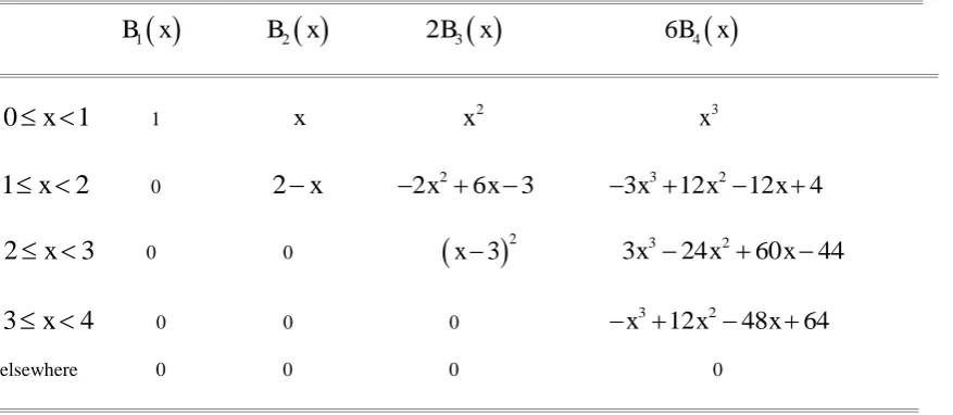
(13)

Cardinal B-splines is an important class of basis functions that can form multiresolution wavelet decompositions (Chui, 1992). The first order cardinal B-spline is the well-known Haar function defined as

 

 





1 0,1

1,

0,1 ,

0,

.

x

B x

otherwise











_{ }



(14)

The second, third and fourth order cardinal B-splines

B x

₂

 

,

B x

₃

 

and

B x

₄

 

are given in Table 1 (Wei and Billings, 2006). For detailed discussions on cardinal B-splines and the associated wavelets, see Chui (1992).

One attractive feature of cardinal B-splines is that these functions are completely supported, and this property enables the operation of the multiresolution decomposition (9) to be much more convenient. For example, the

m th



order B-spline is defined on

 

0,

m

,

thus, the scale and shift indices

j

and

k

for the family of the functions

 

/ 2





,

2

2

,

0 2

.

j j j

j k

x

B

m

x k

x k

m









 

(15)

Assume that the function f x

 

that is to be approximated with decompositions (9) or (11) is defined within

 

0,1 , then for any given scale index (resolution level)

j

,

the effective values for the shift index

,

[image:7.595.71.510.117.308.2]

Table 1 Cardinal B-splines of order from 1 to 4.

 

1

B x

B x

₂

 

2B x

₃

 

6B x

₄

 

0

 

x

1

1 x

x

2

x

3

1

 

x

2

0

2 x





2

x

2



6

x



3



3

x

3



12

x

2



12

x



4

2

 

x

3

0 0



x



3



2

3

x

3



24

x

2



60

x



44

3

 

x

4

0 0 0

 

x

3

12

x

2



48

x



64

elsewhere 0 0 0 0

Note that while the first and second order B-splines B x1

 

and B x2

 

are non-smooth piecewise

functions, which would perform well for signals with sharp transients and burst-like spikes, B-splines of higher order would work well on smoothly changing signals. Motivated by this consideration, this study proposes using multi-wavelet basis functions for time varying ARX and time varying AR model identification. Two examples of the new multi-wavelet based algorithm are given in the following.

Take the B-splines of order from 1 to 4 as an example, and consider the decomposition (13). Let



:

2

j

1 ,



1, 2,

, 4;

m

k m

k

m

 

 





(16)

and

 

_{ }

/ 2





2

2

,

.

m J J

k

x

B

m

x k

k

m









(17)

The time-varying coefficients a ti

 

and

b t

j

 

in model (1) can then be approximated using a combination of functions from the families





k m :m1, , 4;km



. For example, one such

combination can be chosen as,

 

   

 

   

 

   

 

, , ,

q r r

q q r r s s

i i k k i k k i k k

k k k

t

t

t

a t

c

c

c

N

N

N







  













 

   

 

   

 

   

 

, , ,

q r r

q q r r s s

j j k k j k k j k k

k k k

t

t

t

b t

d

d

d

N

N

N







  













(18)

The decomposition (18) can easily be converted into the form of (2), where the collection

 



f t

_j

:

j



1, 2,

,

L



is replaced by the union of the three families:





k q

 

t :kq



,

 

_{ }





_kr t :k_r



and





_k s

 

t :k_s



. Further derivation can then lead to the standard linear regression equation (5). Eq. (18) and Eq. (5) reveal that the initial full regression equation (5) may involve a great number of free time-varying parameters, and least squares type algorithms may fail to produce reliable results for such ill-posed problems. These problems, however, can easily be overcome by performing an effective modified block least mean square algorithm, the resulting recursive coefficient estimates

c

_{i k,} and

d

_{j k,} in Eq. (18) will then be used to recover the time-varying coefficients

a t

_i

 

and

b t

_j

 

in the TVARX and TVAR (without eXogenous inputs) in model (1). Thesimulation results for the latter case shows that the novel method proposed based on multi-wavelet basis functions in this paper was excellent adaptive and tracking abilities.

4.

A Modified Block Least Mean Square Approach

The conventional block LMS algorithm and Normalized LMS (Shynk, 1992; Haykin, 2002) have been proven to be very effective to deal with dynamic regression problems. However, the performance of these algorithms is sensitive to the selection of step sizes and additional noise. In this study we introduce a modified block LMS algorithm, Table 2 presents a summary of the modified block LMS algorithm, where the step size



is divided bythe maximum eigenvalue of the correlation matrix

R

. An important issue that needs to be considered in the design of a block adaptive filter is how to choose the block size

L

.

From Table 2 we observe that the operation of the block LMS algorithm holds true for any interger value of

L

equal to or greater than unity. Nevertheless, the option of choosing the block size

L

equal to the filter length (that is, the number of time-varying parameter coefficients in model (1))

M

is preferred in most applications of block adaptive filtering. This choice has been justified by Clark et al., (1981) based on the following observations:

When

L



M

,

redundant operations are involved in the adaptive process, because then the estimation of the gradient vector (computed over

L

points) uses more input information than the filter itself.

When

L



M

,

some of the tap weights in the filter are wasted, because the sequence of tap inputs is not long enough to feed the whole filter.

It thus appears that the most practical choice is

L



M

.

For

L



1,

the block LMS algorithm reduces to the Normalized LMS (NLMS) algorithm, where

R

is a scalar. For

L



1,

Table 2 is summarized the modified block LMS algorithm, where

R

is a square matrix.

(

0

 



2 /



_max, stability condition) independent of the input data correlation statistics (Goodwin and Sin, 1984; Nagumo and Noda, 1967); ii) for

L



1,

modified block processing of data samples, a block of samples of the filter input and desired output are collected and then processed together to obtain a block of output samples. A good measure of computational complexity in a block processing system is given by the number of operations required to process one block of data divided by the block length. An implementation of the modified block LMS (MBLMS) algorithm is more computationally efficient.

Table 2 Summary of the modified block least mean square algorithm

Definition

   



u

1 ,

u

2 ,



,

input signal samples

   



d

1 ,

d

2 ,



,

desired signal samples correlated with input signal samples

L

block size

,

M

filter length (namely, the number of coefficient parameter in model (1)),

,



step-size,

,

a

a small positive constant,

 





max

max

eig R

,





maximum eigenvalue of the correlation matrix

R



E X



T

   

k X k



,

 

1

 

,

,

 

,

T M

W k

 

_

w k

w

k



_

a vector of weights.

Initial Conditions:

 

ˆ

_{0 ,}

W

a null vector of dimension

M



1.

Computation: at the

k th



iteration, for each new block of

M

input samples, compute

 

























1

1

,

1

1

u kM

u

k

M

X k

u

k

M

u kM













 





_

_











 

 

,

,





1



1



T

,

d k





_

d kM

d

k



M





_

 

   

ˆ

_,

y k



X k W k

 

   

,

e k



d k



y k

 

k

X

T

   

k e k

,





_{  }

_{  }

max

ˆ

₁

ˆ

_.

W k

W k

k

a



_



 





Dimensions:

 

ˆ

W k

M



1

;

X k

 

M M



;

d k

 

M



1

;

y k

 

M



1

; a

1 1



;

 

e k

M



1

;



 

k

M



1

;



1 1



;

R

M M



;



_max

1 1



.

In the present study, the MBLMS algorithm above is used to solve the regression equation (5). This includes a model identification and time-varying parameter estimation. The resultant estimates will then be used to recover the time-varying coefficients

a t

_i

 

and

b t

_j

 

in the TVARX or TVAR (without eXogenous input) model (1).

To determine the proper model size given by (5), the modified generalized cross-validation (GCV) criteria (Orr, 1995; Billings et al, 2007) can be used. The modified generalized cross-validation (GCV) for a set of basis functions for the AR process is given by

 

2

 

ˆ

2

log

p

N

GCV p

N

p







 

_







(19)

where

N

is the length of the data,



ˆ

_p2 is the variance of the model residuals, and

p

is the model size.

5.

Simulation Examples

To verify the performance of the multi-wavelet basis function expansion approach, the performance of the new method for tracking time-varying parameters is studied. Two simulated experiments with different

SNR’s (Signal to Noise Ratio) are presented.

5.1

Example 1

Consider the following time-varying ARX

 

1,1 model,

 

1

  

1



1

  

1

  

y t



a t y t

 

b t u t

 

e t

(20)

The process parameters

a t

₁

 

and

b t

₁

 

are varied in different ways and the output

y t

 

is observed for the system input

u t

 

which was a Pseudo-Random Binary Sequence (PRBS) (Leontaritis, Billings , 1987). The system parameters are estimated using both the NLMS and the modified block LMS (MBLMS) approaches based on multi-wavelet basis functions, respectively.

 

1

0.1

0

0.3

0.9

0.3

0.5

0.5

0.5

0.7

0.6

0.7

1.

t

t

a t

t

t



 





_{ }



 

_

_{ }





_{ }



 

1

0.1

0

0.2

0.5

0.2

0.4

0.8

0.4

0.7

0.3

0.7

1.

t

t

b t

t

t

 





 



 

_{ }





_{ }



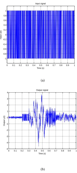
(21)

Figure 1(a) shows the PRBS input signal

u t

 

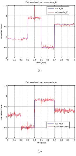
, which is a frequency rich signal. The input signal is of 1 second duration and sampling frequency was 1000 Hz. The output is shown in Figure 1(b) for a noise with SNR=19.40dB. Figure 2(a) and Figure 2(b) show the true and estimated values of parameters

a t

₁

 

and

 

1

b t

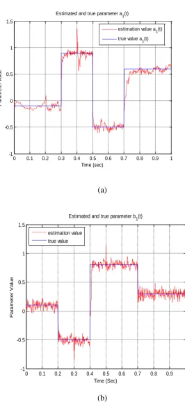
respectively for the noise of SNR=19.40dB using the NLMS algorithm with L1,0.6. The estimated parameters follow the true parameter variations quite well. Figure 3(a) and Figure 3(b) show the true and estimated values of parameters

a t

₁

 

and

b t

₁

 

respectively for the noise of 19.40 dB using the modified block LMS algorithm based on multi-wavelet basis functions with L2,1. The estimated parameters follow the true parameters variations extremely well picking up the abrupt changes very quickly. Estimates were calculated for the given time varying coefficients in (21) and the statistics of the obtained results are presented in Table 3. The standard deviations of the parameter estimates (with respect to the true parameters) are presented in Table 3. The mean absolute error (MAE) of the parameter estimates, with respect to the corresponding true values, are also estimated and shown in Table 3. Compared with the NLMS estimates, the variance for the multi-wavelet basis function method estimates is smaller. The mean absolute error is defined by

   

1

1

_ˆ

,

N k

MAE

a k

a k

N









(22)

where

a k

ˆ

 

represents the estimates of

a k

 

in model (1), and

N

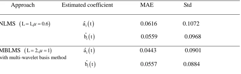
is the length of the data. Table 3 A comparison of the model performance for Example 1 (SNR = 19.40dB).

Approach Estimated coefficient MAE Std

NLMS



L1,0.6



a tˆ1

 

0.0616 0.1072

b tˆ₁

 

0.0559 0.0968 MBLMS



L2,1



a tˆ1

 

0.0443 0.0901 with multi-wavelet basis method b tˆ₁

 

0.0557 0.0884

5.2 Example 2

[image:11.595.114.410.74.147.2] [image:11.595.73.493.549.678.2]

NLMS (L1,0.4), consider a time varying AR

 

2 model that has the following form:

 

1

  

1



2

  

2

  

y t



a t y t

 

a t y t

 

e t

(23)

where

e t

 

is zero-mean Gaussian white noise with a variance 0.2. The time varying parameters were defined by the following expression:

 



 



1

2cos 2

a t





f t

 

2

1,

1,

,1000.

a

t

 

t



(24) where

 

0.29,

333

1, 2,

,333

0.15 0.1sin 2

,

334,

,1000.

333

t

f t

t

t

N













_







_







_

_

_



(25)

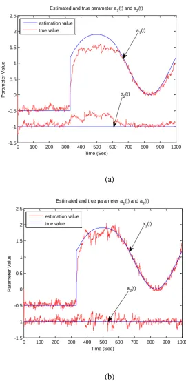
A sharp transition at t333 was purposely selected to test and verify the new approach when the time-vary parameter is sharply varied from a square-shaped to a sinusoidal shape. Gaussian white noise was added to the system output of (23) so that the signal-to-noise ratio was 13.34 dB. The determination of the model order of two based on multi-wavelet basis functions was calculated using (19). Figure 4 shows the performance of the parameter estimation using the MBLMS (L2,0.25) method coupled with the multi-wavelet basis function algorithm and the traditional NLMS (L1,0.4) method for time varying parameter estimation with a noise of SNR=13.34dB. The method based on the new multi-wavelet basis function algorithm outperforms that of NLMS (L1,0.4). The results with the new multi-wavelet basis functions are impressive because the algorithm tracks three distinct waveforms: a constant value, an abrupt change, and the sinusoidal waveform.

As in previous example, both the standard deviations and the mean absolute error for the parameter estimates are calculated and these are presented in Table 4. Clearly, compared with the NLMS estimates, both the variance and the mean absolute error for the multi-wavelet basis function method estimates are much smaller.

Table 4 A comparison of the model performance for Example 2 (SNR = 13.34 dB).

Approach Estimated coefficient MAE Std

NLMS



L1,0.4



a tˆ1

 

0.1507 0.1909

a tˆ₂

 

0.1433 0.1417

MBLMS



L2,0.25



a tˆ1

 

0.0802 0.1221

with multi-wavelet basis method a tˆ₂

 

0.0719 0.0988

6.

Conclusions

Time-varying parameters in both ARX and AR models have been estimated using a new MBLMS algorithm introduced in this study. Parameter variations including both fast and abrupt changes have been considered. Performance measures of the estimated parameters have been calculated under different noise conditions. The experimental simulations indicate that, even up to noise level of 13.3433 dB, the new approach based on multi-wavelet basis functions and the MBLMS algorithm gives much better results for fast and abrupt changing parameters than the method which uses the traditional normalized least mean square (NLMS) algorithm directly. Furthermore, from the results above, it can be concluded that time-varying systems can be modelled using a time varying ARX or a time varying AR model and the identification problem of modelling fast and abrupt changing time-varying parameters is possible with good accuracy. The results are satisfactory for both fast and abrupt changing parameters even in the presence of noise.

The wavelet method is especially powerful for nonstationary signal analysis. Further research in this direction will focus on extracting features of biomedical signals using wavelet methods and time varying ARX or AR modelling methods. The results will then be applied to modelling and tracking time-varying signals that consist of both slow and fast time-varying dynamics.

Acknowledgements

Y. L. acknowledges the support provided by the University of Sheffield under the scholarship scheme and the authors gratefully acknowledge that this work was supported by the Engineering and Physical Sciences Research Council (EPSRC), U. K and the European Research Council (ERC).

References

[1] Billings, S. A., Wei, H. L. and Balikhin, M. A. (2007), ‘Generalized multiscale radial basis function networks’, Neural

Networks, 20, 1081–1094.

[image:13.595.73.496.114.244.2]

functions’, IEEE trans. Biomedical Engineering, 52, 956-960.

[3] Chui, C. K., An Introduction on Wavelets, Boston: Academic Press, 1992.

[4] Clark, G. A., Mitra, S. K. and Parker, S. R. (1981), ‘Block implementation of adaptive digital filters’, IEEE Trans.

Circuits Syts. Vol. CAS-28.

[5] Fahmida, N. C. (2000), ‘Input-output modelling of nonlinear systems with time-varying linear models’, IEEE

Transactions on Automatic Control, 45, 1355-1358.

[6] Goodwin, G. C. and Sin K. S., Adaptive Filtering, Prediction, and Control, Englewood Cliffs, NJ: Prentice-Hall, 1984.

[7] Haykin, S., Adaptive Filter Theory, 4th ed., Pearson Education, 2002.

[8] Kokangul, A. (2008), ‘A combination of deterministic and stochastic approaches to optimize bed capacity in a hospital

unit’, Computer Methods and Programs in Biomedicine,90, 56-65.

[9] Leontaritis I, Billings S A (1987), ‘Experimental design and identifiability for nonlinear systems’, Int J Control, 18,

189-202

[10] Mallat, S. G. (1989), ‘A theory for multiresolution signal decomposition: the wavelet representation’, IEEE

Transactions on Pattern Analysis and Machine Intelligence, 11, 674-693.

[11] Nagumo, J. and Noda, A. (1976), ‘A learning method for system identification’, IEEE Trans. Automat. Cont., 12,

282-287.

[12] Orr, M. J. (1995), ‘regularization in the selection of radial basis function centers’, Neural Computation, 7, 606-623.

[13] Shynk, J. J. (1992), ‘Frequency-domain and multirate adaptive filtering’, IEEE Signal Processing Mag., 9, 14-37.

[14] Wei, H. L. and Billings, S. A. (2006), ‘An efficient nonlinear cardinal B-spline model for high tide forecasts of at the Venice lagoon’, Nonlinear Processes in Geophysics, 13, 577-584.

[15] Wei, H. L. and Billings, S. A. (2002), ‘Identification of time-varying systems using multiresolution wavelet models’,

International Journal of Systems Science, 33, 1217-1228.

[16] Wei, H. L., Liu, J and Billings, S. A. (in press), ‘Time-Varying Parametric Modelling and Time-Dependent Spectral

Characterization with Application To EEG Signal Using Multi-Wavelets’, To appear in International Journal of

Modelling, Identification and Control.

[17] Zou, R., Wang, H. and Chon, K. H. (2003), ‘A robust time-varying identification algorithm using basis functions’,

0 0.1 0.2 0.3 0.4 0.5 0.6 0.7 0.8 0.9 1 -1

-0.8 -0.6 -0.4 -0.2 0 0.2 0.4 0.6 0.8 1

Time (s)

In

p

u

t

u

(t

)

Input signal

0 0.1 0.2 0.3 0.4 0.5 0.6 0.7 0.8 0.9 1 -5

-4 -3 -2 -1 0 1 2 3 4

Time (s)

O

u

tp

u

t

y

(t

)

Output signal

(a)

[image:15.595.153.412.109.686.2]

(b)

(a)

[image:16.595.150.417.106.696.2]

(b)

Figure 2 Time-varying parameter estimation using a normalized LMS approach (NLMS) with L1,0.6

and SNR of 19.4024 dB for Example 1. (a) Estimated and true parameter a1(t), and (b) Estimated and true

parameter b1(t).

0 0.1 0.2 0.3 0.4 0.5 0.6 0.7 0.8 0.9 1 -1

-0.5 0 0.5 1 1.5

Time (sec)

P

a

ra

m

e

te

r

v

a

lu

e

Estimated and true parameter a₁(t)

estimation value a

1(t)

true value a

1(t)

0 0.1 0.2 0.3 0.4 0.5 0.6 0.7 0.8 0.9 1

-1 -0.5 0 0.5 1 1.5

P

a

ra

m

e

te

r

V

a

lu

e

Time (Sec)

Estimated and true parameter b₁(t)

(a)

[image:17.595.161.423.122.660.2]

(b)

Figure 3 Time-varying parameter estimation using a MBLMS approach based on multi-wavelet basis function with L2,1 and SNR of 19.4024 dB for Example 1. (a) Estimated and true parameter a1(t), and (b) Estimated and true parameter. b1(t).

0 0.1 0.2 0.3 0.4 0.5 0.6 0.7 0.8 0.9 1 -1

-0.5 0 0.5 1 1.5

Time (Sec)

P

a

ra

m

e

te

r

V

a

lu

e

Estimated and true parameter a₁(t) true a₁(t) estimated a₁(t)

0 0.1 0.2 0.3 0.4 0.5 0.6 0.7 0.8 0.9 1 -1

-0.5 0 0.5 1 1.5

Time (sec)

P

a

ra

m

e

te

r

V

a

lu

e

Estimated and true parameter b₁(t)

(a)

[image:18.595.138.409.90.645.2]

(b)

Figure 4 Comparison of simulation example with MBLMS (L2,0.25) based on multi-wavelet basis function with a NLMS (L1,0.4) for time varying parameters estimation with SNR of 13.3433 dB for Example 2, (a) actual (solid lines) and estimated (dotted lines) model parameters with a NLMS (L1,0.4) method, (b) actual (solid lines) and estimated (dotted lines) model parameters with MBLMS (L2,0.25) based on multi-wavelet basis functions approach

0 100 200 300 400 500 600 700 800 900 1000 -1.5

-1 -0.5 0 0.5 1 1.5 2 2.5

Time (Sec)

P

a

ra

m

e

te

r

V

a

lu

e

Estimated and true parameter a₁(t) and a₂(t)

a₁(t)

a₂(t) estimation value

true value

0 100 200 300 400 500 600 700 800 900 1000 -1.5

-1 -0.5 0 0.5 1 1.5 2 2.5

Time (Sec)

P

a

ra

m

e

te

r

V

a

lu

e

Estimated and true parameter a₁(t) and a₂(t)

a

1(t)

a

2(t)