Using Technomatix Simulation Software as a Validation Tool for Plant Layout of an Off Highway Vehicle: Frame Assembly

(1)

International Journal of Innovative Technology and Exploring Engineering (IJITEE) ISSN: 2278-3075, Volume-8 Issue-12, October 2019



Abstract: Development of any new product envisages strenuous and discreet efforts at various levels of designing and manufacturing. A typical development involves the designing, virtual validation manufacturing and assembly planning. These phases play a remarkable role in the lucrative advancement of the new product. This project, italicizes on the Design and Plant Layout phases including the virtual validations using the latest technologies developed in the recent times. For this purpose, a product contemplated is the frame of an off-highway vehicle in which the new design of the frame assembly has been generated, validated the same against the standard working condition specified by authorities, generated the plant layout for the assembling of this frame structure and validated the generated plant layout using plant layout validation software Technomatix to optimize the same for better and optimum results

Keywords:LARGE scale optimization, Production; Simulation, Technomatix

I. INTRODUCTION

This proposition parades the methodology on how in modern day technology the complete manufacturing process can be done with the help of the most suitable software technologies from the design stage to the final manufacturing plant layout phase.

During this work, concentration is given on the design, validation and manufacturing plant layout. More specifically on the design stages as these have some of the major activities involved in the development stage. Moreover, these sectors have witnessed much advancement in the recent times. Also, the part level manufacturing procedure is assumed to be done separately and casted aside for the project.

This project designed an off-highway vehicle frame as the basis for the study, which is made up of a tubular structure welded together. The alpha of the field is the designing of the vehicle and validating the vehicle using the Nastran Software for both the static loading condition as well as the vibration loading conditions.

Revised Manuscript Received on October 05, 2019.

M. Shameer Basha*, Department of Mechanical Engineering, Unayzah College of Engineering Qassim University, Qassim51911, SaudiArabia : [email protected] , [email protected]

Ali Sulaiman Alsagri, Department of Mechanical Engineering, Unayzah College of Engineering Qassim University, Qassim 51911, Saudi Arabia alsagria1@ gmail.com, [email protected]

Syed Azam Pasha Quadri, Department of Mechanical Engineering, Lords Institute of Engineering and Technology, Hyderabad, Telangana, 500091 [email protected]

S. Raghavendra, Department of Mechanical Engineering, Lords institute of Engineering and Technology, Hyderabad, Telangana, [email protected]

Mohd Yousuf Ahmed, Department of Mechanical Engineering, Lords institute of Engineering and Technology, Hyderabad, Telangana, 500091 [email protected]

The next leg of the project deals with the manufacturing simulation at assembly layout to identify the most suitable plant layout for achieving the optimum product output, a targeted output of 1500 pieces per month.Little iteration was performed to identify the same and the final conclusion is derived. The detailed project gives the step by step details on the entire process followed.

MAJOR ACTIVITIES INVOLVED IN THE PROJECT EXECUTION

The project consists of the following stages: 1 .Design of the Vehicle Frame Assembly.

2. Validating the Design for its structural performance for i. Static Loading conditions.

ii. Dynamic Loading conditions. 3. Generating the Assembly sequence.

4. Validating the Plant Layout to verify the throughput. 5.Optimizing the Plant Layout for increase of the output to meet the throughput.

6. Conclusion.

1. Design of the vehicle frame assembly

With the available information and the literature, the design is frozen as a modular structure, in which the entire frame has been divided into 6 whole parts. All these parts will get manufactured separately at various locations and they will get assembled to make the entire frame assembly. Fig 1 shows the schematic design of the Off-highway vehicle designed for the study purpose and the frame assembly with various sub parts is shown. UG NX software is used for the designing of 3D Model and Assembly.

Fig.1.Schematic Diagram of the Off-Highway vehicle.

Using Technomatix Simulation Software as a

Validation Tool for Plant Layout of an

Off-Highway Vehicle: - Frame Assembly

(2)

- Frame Assembly

II. VALIDATING THE DESIGN FOR ITS

STRUCTURAL PERFORMANCE

One of the main steps to eliminate the rework in the design is to validate before it goes to manufacturing. In any typical product life cycle, there are various steps involved as shown in Figure 2.

Fig.2. Flow Diagram showing Product development stages.

Each stage in this process involved abundantly large amount of time and money.

If the product fails during the test, then it is equivalent to the stage 1 of product development as all the aforementioned activities have to be redone which would take the same amount of time.

So Virtual validation of the design using CAE technique plays a major role in any development activity of any product development cycle. This is due to the fact that many new CAE technologies have been developed in the recent times to cope with the demand from the industry to cater to various requirements. Following are the various virtual validation testing’s for which the product is intended to work satisfactorily.

2.1. Functional requirements of the Frame Assembly The Frame structure has to with stand various loading conditions namely

a) Static loading conditions. b) Vibration loading conditions. c) Sudden Impact loading conditions.

In addition to the various other loading conditions which will apply due to changes in the atmospheric conditions.

a. Static loading condition

For the off-road vehicle, it’s decided to use the static loading condition as follows.

Person weight: 100 kgs.

Factor of Safety for the sudden loading conditions: 2.5 times. Static loading conditions: 250 kgs.

b. Vibration loading condition

The vibration loading condition is taken from the available ARAI standard condition for automotive performance condition, given below.

The Frame Assembly is subjected to excitation load of 1g in the X, Y & Z directions for a frequency range of 10 Hz to 40 Hz. A damping coefficient of 0.02 (i.e. 2%) was used. c. Sudden impact loading

The Impact Loading conditions are assumed to be considered in the FOS and are neglected for the scope of the project.

[image:2.595.299.556.100.365.2]

Considering these above loading conditions, the design of the Frame Assembly been generated and is finalized for the further study purpose.

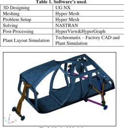
Table 1. Software’s used.

3D Designing UG NX

Meshing Hyper Mesh

Problem Setup Hyper Mesh

Solving NASTRAN

Post-Processing HyperView&HyperGraph Plant Layout Simulation Technomatix – Factory CAD and

Plant Simulation

Fig.3. Meshed Model. Table 2. Features of Meshed Model. No. of Elements 74741

No. of Nodes 63496

Thickness of Frame (mm) 3 Mass of structure (kg) 374 Lump mass (kg) 250 Total Mass of structure (kg) 624

Table 3. Material Properties (Steel). Density(Tones/mm3) 7.89E-09

[image:2.595.301.553.102.735.2]

Elastic Modulus (MPa) 210000 Poisson’s Ratio 0.3 Yield Strength (MPa) 240

Fig.4. Boundary Conditions applied on Frame Assembly. 2.2. a Static Analysis Results

[image:2.595.53.280.133.285.2]

(3)

Fig.5. Stress Plot due to static analysis.

[image:3.595.59.284.41.791.2]

Fig.6. Stress Plot due to static analysis. ii. Displacement Plot

[image:3.595.302.548.48.295.2]

Fig.7.Displacement Plot due to static analysis.

Fig.8. Displacement Plot due to static analysis. Table 4. Results Conclusion: Static analysis. S.No. Load Case Stress

(MPa)

Displacement (mm)

1 Static Self-weight

Analysis 48.78 0.55

2.2.b Vibration Analysis

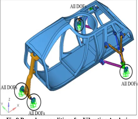
[image:3.595.309.545.350.553.2]

Modal Analysis: Modal Analysis has been carried out to find out the natural frequencies of the Car Assembly.

Fig.9.Boundary conditions for Vibration Analysis. Frequency Range: up to 40 Hz, following modes been identified.

Table 5. Frequency modes. Mode No Frequency (Hz)

1 33.19

2 36.71

(4)

[image:4.595.67.549.44.508.2]

- Frame Assembly

[image:4.595.311.538.297.521.2]

Fig.10. 1st Mode Frequency Result. 2nd Mode frequency: Frequency @36.71Hz

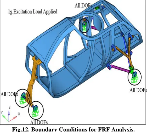
Fig.11. 2nd Mode Frequency Result 2.3 Frequency Response Function (FRF) Analysis FRF analysis has been carried out to find Maximum Stress and Maximum displacement, when an excitation load of 1g is applied in X, Y & Z directions on the Car Assembly.

Fig.12. Boundary Conditions for FRF Analysis. The Car Assembly is subjected to excitation load of 1g in the X, Y & Z directions for a frequency range of 10 Hz to 40 Hz. A damping coefficient of 0.02 (i.e. 2%) was used.

[image:4.595.48.291.495.711.2]

Case a: Excitation in X axis at 33.19 Hz

Fig.13.FRF Analysis results – Case a – Stress Plot.

Fig.14.FRF Analysis results – Case a – Displacement Plot.

Load Case b: Excitation in Y-axis at 36.71 Hz

[image:4.595.316.535.541.712.2]

(5)

Fig. 16. FRF Analysis results – Case b – Displacement Plot.

Load Case c: Excitation in Z-axis at 33.19 Hz

[image:5.595.47.289.29.539.2]

Fig. 17. FRF Analysis results – Case c – Stress Plot.

[image:5.595.317.533.73.796.2]

Fig. 18.FRF Analysis results – Case c – Displacement Plot. Table 6. Result Analysis

S.

No Load Case

Frequen cy (Hz)

Stres s (MPa )

Displacemen t

(mm) 1 X- direction 33.19 98.24 1.41 2 Y-direction 36.71 66.01 1.18 3 Z-direction 33.19 9.79 0.32

Conclusion on the FEA Results

From the CAE results it’s evident that the design is robust; the stresses and the displacement values generated both in the case of Static analysis condition and in vibration condition are well within the acceptable limit of the material yield stress values. So the model is certified for the manufacturing purpose.

III. GENERATING THE ASSEMBLY SEQUENCE

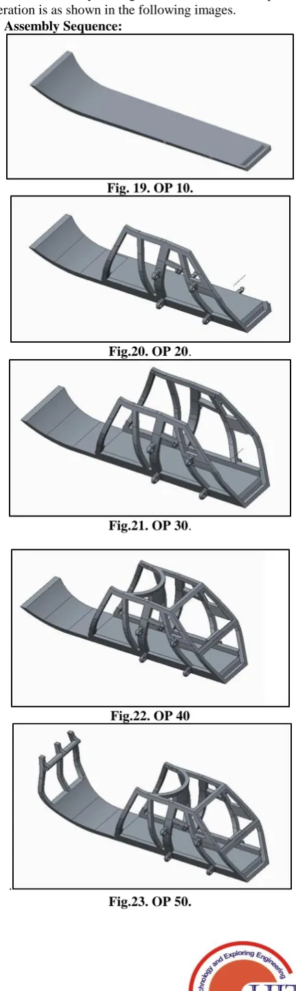
The Frame Assembly is designed as 6 different parts, which can be assembled by bolting with each other. The sequence of operation is as shown in the following images.

3.1 Assembly Sequence:

Fig. 19. OP 10.

Fig.20. OP 20.

Fig.21. OP 30.

Fig.22. OP 40

.

[image:5.595.43.283.553.660.2]

(6)

[image:6.595.65.275.50.197.2]

- Frame Assembly

Fig.24. OP 60.

The above Fig 19 to Fig 24 will give the details on how the assembly is going to happen, in step wise.

OP 10: Fixing the Bottom Frame Member (BFM). OP 20: Welding the LH Side Frame Member (LHFM). OP 30: Welding the RH Side Frame Member (RHFM). OP 40: Welding the Front Frame Member (FFM). OP 50: Welding the Rear Frame Member (RFM). OP 60: Welding the Top Frame Member (TFM).

IV. VALIDATING THE PLANT LAYOUT TO VERIFY THE THROUGH OUTPUT

The next leg of the activity is to generate the plant layout using the existing plant layout software and validating the plant layout for the throughput it is planned .

As noticed in the assembly timings, there are 5 stations in all in which the entire assembly of the frame assembly is going to be completed. It is understood that the designed plant layout is a stationary worker and moving assembly line.

Following aspects have to be considered while constructing the plant (and layout generation)

• Expected throughput from the plant • Line Balancing for optimized output

• Bottlenecks in the proposed plant layout and its buffers • Probable down time and its buffers

• Optimum utilization of the resources, including manpower So to evaluate the performance of the proposed plan of the plant layout, it is decided to assess the same using Factory CAD and Factory Simulation modules of the Digital Manufacturing module of Technomatix software, developed by Siemens Software Ltd.

4.1 About Technomatix Software

Technomatix® Plant Simulation software enables the simulation and optimization of production systems and processes. Using Plant Simulation, you can optimize material flow, resource utilization and logistics for all levels of plant planning from global pro¬duction facilities, through local plants, to specific lines.

With increasing costs, time limit pressures limitation in production, and ongoing globalization, logistics has become a key factor in the success of a company. The need to deliver JIT (just-in-time)/ JIS (just-in-sequence), introduce Kanban, plan and build new, sustainable production facilities, and manage global production networks requires objective decision criteria to help management to evaluate and compare alternative approaches.

4.2 Designing the Plant Layout using Factory CAD

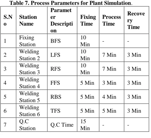
Following are the process parameters based on which the plant layout been designed.

i. There are six stations in which does the welding operations been performed from OP 10 to OP 60.

ii. It is assumed that the parts are tested for the quality before they are brought to the final assembly line. There will be some visual inspection done by the Q.C in-charge before they are sent for the next operation.

iii. Fixing station is the place where the bottom frame will be mounted in the fixture. There will be no welding in this station.

iv. All the layout is assumed to be mounted on a conveyer. The conveyer is operated at the specified time intervals based on the instruction from the users.

v. At the end of the welding of all the parts, final Q.C will be done on the final frame assembly.

vi. Rejection % due to weld failures are considered as 10%. vii. Downtime of the equipment is consideredas 10% of total available time.

viii. Only one shift (8Hrs) working is considered. ix. Conveyer speed of 0.1meter for sec.

x. Working week is considered as Monday to Saturday. Table 7. Process Parameters for Plant Simulation. S.N o Station Name Paramet er Descripti on Fixing Time Process Time Recove ry Time 1 Fixing

Station BFS

10

Min - -

2 Welding

Station 2 LFS

10

Min 7 Min 3 Min 3 Welding

Station 3 RFS

10

Min 7 Min 3 Min 4 Welding

Station 4 FFS 5 Min 3 Min 3 Min 5 Welding

Station 5 RBS 5 Min 4 Min 3 Min 6 Welding

Station 6 TFS 5 Min 5 Min 3 Min 7 Q.C

Station Q.C Time 15

Min - -

V. OPTIMIZING THE PLANT LAYOUT FOR

INCREASE OF THE OUTPUT TO MEET THROUGHPUT

[image:6.595.304.565.322.559.2]

(7)

Fig.25. Iteration 1 Plant Layout

Plant Layout in Plant Simulation Software

Fig.26. 3D Plant Layout in Plant Simulation.

Fig.27. Resource Statistics.

From the above Analysis, it is found that:

i. Station 2 and station 3, seem to be much occupied whereas rest of the stations are comparatively free.

ii. Efficiency of each station is as shown above. It is identified that there is a large amount of idle time.

iii. Station 2 and 3 have become the bottleneck for the layout which caused the delay in the process.

iv. Total throughput is only 754 pieces and total entries are 854 pieces.

With these inputs, its discussed and understood that the plant layout should be changed to get the desired outputs and eliminating the bottlenecks in the system.

After the through study and some more iterations of the system, following new plant layout been proposed and decided to study.

After some of the modification iterations, the solution reached equilibrium where the required output is being achieved and the same is given below.

5.2 Iteration 2: Modified Layout

Following Fig is showing the optimized layout, proposed to achieve the required throughput with much balanced plant layout.

Fig.28. Iteration 1 Plant Layout.

All the process parameters remained same as the iteration 1. With the analysis of the Iteration 2, following are the outputs identified.

(8)

- Frame Assembly

Fig.30. 3D Plant Layout in Plant Simulation.

The total throughput increased to 826 pieces against the iteration1 throughput of 754 pieces with increase of 10% output.

From the analysis, it is understood that the bottleneck in this layout is in Q.C arrangement as much amount parts are being held at this station. So it is decided to add one more Q.C station and see the output.

5.3 Iteration 3: With 2 Q.C lines added

Following layout shows the modified layout in which 2 Q.C lines added in it.

Proposed Plant Layout

Fig.32. Iteration 3 Plant Layout.

Fig.33. Iteration 3 Plant Layout. 3D Plant Simulation layout

Fig.34.3D Plant Simulation layout.

This is the best possible output and it is the much optimized solution with these inputs.

VI. CONCLUSION

From the above studies, optimized design is achieved for the output of 1652 pieces per month against the target of 1500 pieces. With a downtime of 10%, this is exactly meeting the target requirement of the total target production output. Also, it is found and understood that the layout is perfectly balanced with minimal waiting time at each station.

(9)

FURTHER SCOPE TO WORK

The plant layout can further be optimized with many other possible solutions to achieve further increase in the throughput. As the total output requirement is only 1500 pieces per month, the analysis iteration is stopped at this limit. Table 8. Nomenclature

CAE Computer Aided Engineering.

BFM Bottom Frame Member.

LHFM Left Hand Side Frame

Member.

RHFM Right Hand Side Frame

Member.

FFM Front Frame Member.

RFM Rear Frame Member.

TFM Top Frame Member.

FRF Frequency Response Function.

ARAI Automotive Research

Association of India. REFERENCES

1. Finite Element Procedures by K.J.Bathe.

2. Basics of Finite Element Analysis by Ken Yusuffie.

3. Introduction to the Finite Element Method by EvgenyBarkanov. 4. Plant Simulation software details by Siemens.

5. Pochamarn Tearwattanarattikal*, Suwadee Namphacharoen and Chonthicha Chamrasporn “Using ProModel as a simulation tools to assist plant layout design and planning: Case study plastic packaging factory.