Applicability and consequences of the integration of alternative models for CO2 transfer velocity into a process based lake model

https://doi.org/10.5194/bg-16-3297-2019 © Author(s) 2019. This work is distributed under the Creative Commons Attribution 4.0 License.

Applicability and consequences of the integration of alternative

models for CO

2

transfer velocity into a process-based lake model

Petri Kiuru1,2, Anne Ojala3,4,5, Ivan Mammarella6, Jouni Heiskanen6,7, Kukka-Maaria Erkkilä6, Heli Miettinen8, Timo Vesala4,6, and Timo Huttula1

1_{Finnish Environment Institute, Freshwater Centre, Survontie 9A, 40500 Jyväskylä, Finland}

2_{University of Jyväskylä, Department of Physics, P.O. Box 35, 40014 University of Jyväskylä, Jyväskylä, Finland} 3_{Faculty of Biological and Environmental Sciences, Ecosystems and Environment Research Programme,}

University of Helsinki, Niemenkatu 73, 15140 Lahti, Finland

4_{Institute for Atmospheric and Earth System Research/Forest Sciences, Faculty of Agriculture and Forestry,} University of Helsinki, P.O. Box 27, 00014 Helsinki, Finland

5_{Faculty of Biological and Environmental Sciences, Helsinki Institute of Sustainability Science,} University of Helsinki, Helsinki, Finland

6_{Institute for Atmospheric and Earth System Research/Physics, Faculty of Science, University of Helsinki,} P.O. Box 68, 00014 Helsinki, Finland

7_{ICOS ERIC Head Office, Erik Palménin aukio 1, 00560 Helsinki, Finland}

8_{Faculty of Biological and Environmental Sciences, University of Helsinki, P.O. Box 65, 00014 Helsinki, Finland}

Correspondence:Petri Kiuru ([email protected]) Received: 14 March 2019 – Discussion started: 9 April 2019

Revised: 24 July 2019 – Accepted: 6 August 2019 – Published: 4 September 2019

Abstract.Freshwater lakes are important in carbon cycling, especially in the boreal zone where many lakes are super-saturated with the greenhouse gas carbon dioxide (CO2) and emit it to the atmosphere, thus ventilating carbon originally fixed by the terrestrial system. The exchange of CO2between water and the atmosphere is commonly estimated using sim-ple wind-based parameterizations or models of gas transfer velocity (k). More complex surface renewal models, how-ever, have been shown to yield more correct estimates ofkin comparison with direct CO2 flux measurements. We incor-porated four gas exchange models with different complex-ity into a vertical process-based physico-biochemical lake model, MyLake C, and assessed the performance and ap-plicability of the alternative lake model versions to simulate air–water CO2fluxes over a small boreal lake. None of the in-corporated gas exchange models significantly outperformed the other models in the simulations in comparison to the measured near-surface CO2concentrations or respective air– water CO2fluxes calculated directly with the gas exchange models using measurement data as input. The use of more complex gas exchange models in the simulation, on the

con-trary, led to difficulties in obtaining a sufficient gain of CO2 in the water column and thus resulted in lower CO2 fluxes and water column CO2concentrations compared to the re-spective measurement-based values. The inclusion of sophis-ticated and more correct models for air–water CO2exchange in process-based lake models is crucial in efforts to properly assess lacustrine carbon budgets through model simulations in both single lakes and on a larger scale. However, finding higher estimates for both the internal and external sources of inorganic carbon in boreal lakes is important if improved knowledge of the magnitude of CO2 evasion from lakes is included in future studies on lake carbon budgets.

1 Introduction

con-tribution of lakes to the global carbon budget is recognized to be substantial in comparison to the role of marine and terres-trial ecosystems as global carbon sinks, but quantitative esti-mates of the global contribution of lakes and other inland wa-ters show significant variation (Cole et al., 2007; Battin et al., 2009; Tranvik et al., 2009). Atmospheric CO2exchange be-tween lakes and the atmosphere is one of the key processes needed to be determined in constructing carbon budgets of lakes and in evaluating the role of lakes in global carbon cy-cling.

The exchange of weakly soluble gases, like CO2and oxy-gen, across the air–water interface is often modeled as a boundary-layer process in which the gas flux is proportional to the gas concentration gradient at the interface. The pro-portionality factor k is known as the gas transfer veloc-ity. In many long-used models for the gas transfer velocity, or gas exchange models, k is parameterized as a function of wind speed alone (Wanninkhof, 1992; Cole and Caraco, 1998). However, direct measurements of air–water CO2 ex-change using the eddy covariance (EC) method (Jonsson et al., 2008; MacIntyre et al., 2010; Heiskanen et al., 2014) have resulted in higher estimates of k compared to wind-based gas exchange models. For weakly soluble gases,k de-pends mainly upon turbulence in near-surface water (Baner-jee, 2007), which is not generated merely by wind. Near-surface turbulence is initiated predominantly by wind shear and negative buoyancy flux related to thermal convection in-duced by surface heat loss (Imberger, 1985). Buoyancy flux is relatively more important in small, wind-sheltered lakes, and parameterizations of the gas transfer velocity that are based solely on wind speed may not be applicable under such conditions (Read et al., 2012). Turbulence-driven gas exchange models have been shown to be well in accordance with in situ measurements ofk(e.g., Zappa et al., 2007; Va-chon et al., 2010).

In surface renewal models, k is calculated as a function of the turbulent kinetic energy dissipation rateε, which pro-vides an indication of the intensity of near-surface turbulence (MacIntyre et al., 1995). Kinetic energy dissipation can be due to viscous and thermal processes, and εis thus depen-dent on wind shear and convective heat flux (Lombardo and Gregg, 1989). Wind shear is characterized by wind-induced water-side friction velocity. The water-side friction veloc-ity can be estimated from the atmospheric friction velocveloc-ity, which can be measured directly (Mammarella et al., 2015) or calculated by bulk formulas using meteorological variables (Fairall et al., 1996). Heat-induced turbulence is generated if the surface heat flux is directed out of the lake. If measure-ments of the components of surface heat flux are not avail-able, they can also be estimated using bulk formulas (Fairall et al., 1996).

Global estimates of carbon emissions from lakes of-ten use conservative estimates of CO2 fluxes or models that yield potentially underestimated values for k, lead-ing to low estimates of CO2 fluxes (e.g., Cole et al., 2007;

Raymond et al., 2013). Thus, revised estimates of lacustrine CO2emissions will require higher net ecosystem production in the land-based ecosystems of the terrestrial biosphere to close the global carbon balance (Battin et al., 2009). Many studies concerning modeling lake carbon balance (e.g., Bade et al., 2004; McDonald et al., 2013) or the determination of lake carbon budgets (e.g., Sobek et al., 2006; Stets et al., 2009; Chmiel et al., 2016) also use simple wind-based mod-els fork. Potential subsequent underestimates in carbon ef-flux may have consequences for the interpretation of carbon budgets in single lakes (Dugan et al., 2016). A higher ef-flux may result in a reevaluation of the amount of net ecosys-tem production in lakes, or it can mean that external carbon sources are inadequately accounted for in lake carbon bud-gets.

The efflux of CO2from a lake is sustained mainly by in-lake CO2 production through the bacterial or photochemi-cal degradation of organic matter in the water column or in sediment. Widely across the boreal zone, the importance of the degradation of allochthonous organic matter as an inor-ganic carbon source in lakes is conspicuous (Jonsson et al., 2001; Sobek et al., 2003). Also, the direct loading of terres-trially produced dissolved inorganic carbon (DIC) through surface water and groundwater inflows may lead to high CO2 concentrations in some lakes (Maberly et al., 2013; Weyhen-meyer et al., 2015; Einarsdóttir et al., 2017).

2 Materials and methods

2.1 Modeling approach

In this study, we assessed the applicability of four different models for the gas transfer velocity, referred to as gas ex-change models, to a process-based physico-biogeochemical lake model, MyLake C. The four gas exchange models were selected because their performance in estimating air–water CO2 fluxes in a small boreal lake has been extensively as-sessed in previous studies by Heiskanen et al. (2014), Mam-marella et al. (2015), and Erkkilä et al. (2018) by comparing the calculated fluxes with direct CO2flux measurements. The models include (1) the widely applied experimental wind-based regression formula by Cole and Caraco (1998), (2) a boundary-layer model developed by Heiskanen et al. (2014), (3) a surface renewal model by Tedford et al. (2014), and (4) a regression model by MacIntyre et al. (2010).

2.1.1 Parameterization of air–water gas exchange

The flux of CO2 between water and the atmosphere,FCO2,

can be parameterized as the product of the CO2 concentra-tion difference between the surface water and the atmosphere with the gas transfer velocityk(Cole and Caraco, 1998):

FCO2=αk(Cw−Ceq), (1)

whereCwis the CO2concentration in the surface water be-low the air–water interface,Ceqis the equilibrium concentra-tion of CO2, that is, the water column CO2concentration in the state of equilibrium with the overlying atmosphere, and αis the chemical enhancement factor applicable for reactive gases, such as CO2. Gas fluxes from water to the atmosphere are thus defined to be positive. If a lake is nonalkaline,αcan be assumed to be 1 (Cole and Caraco, 1998). The equilibrium concentration is calculated by Henry’s law as

Ceq=KHχ pa, (2)

whereKH is the temperature-dependent aqueous-phase sol-ubility (also known as the Henry’s law constant) of CO2at surface water temperature,χ is the mole fraction of the gas in the atmosphere, andpais the atmospheric pressure.

The gas transfer velocitykcan be simply parameterized as a function of wind speed alone, or more complex models can be applied to describe the air–water gas exchange process or the near-surface turbulence that governs the gas exchange. In each of the four gas exchange models assessed in this study, the parameterization ofkis made using a different combina-tion of parameters. The parameters of each model and their units are listed in Table 1. With the exception of the simple wind-based model by Cole and Caraco (1998), near-surface turbulence is driven in the models by both wind shear and thermal convection promoted by heat loss from the surface.

Convection-driven turbulence occurs when surface heat flux is directed out of the lake, that is, when the buoyancy

flux is negative (MacIntyre et al., 2010). The buoyancy flux βis defined as (Imberger, 1985)

β=gαwQeff ρwcpw

, (3)

whereg is the gravitational acceleration,αw is the thermal expansion coefficient of water,Qeffis the effective heat flux, ρwis the density of water, andcpw is the specific heat

capac-ity of water. The effective heat flux is defined as Qeff=QS+QSW(0)+QSW(zAML)

− 2 zAML

zAML

Z

0

QSW(z)dz, (4)

whereQS=QH+QL+QLW is the net surface heat flux, QH is sensible heat flux,QL is latent heat flux,QLWis net longwave radiation,QSWis shortwave radiation, andzAML is the depth of the actively mixing layer (AML) (Imberger, 1985). All heat fluxes from the atmosphere into the lake are defined as positive. The last three terms in the equation repre-sent the fraction of shortwave radiation that is trapped within the AML, denoted as QSW,AML. The attenuation of short-wave radiation at depthzin the water column can be calcu-lated using the Beer–Lambert law:

QSW(z)=QSW(0)e−KLz, (5)

whereKL is the total attenuation coefficient of shortwave radiation. The AML is defined as the near-surface layer in which the water column temperature is within a certain range, usually 0.02◦_{C, of the temperature at the air–water}

interface (MacIntyre et al., 2001). The buoyancy flux is pos-itive when the near-surface water is heating and negative un-der cooling conditions.

In the boundary-layer model developed by Heiskanen et al. (2014), near-surface turbulence is parameterized through wind-induced and convection-induced water-side velocity scales, which are characterized by the wind-induced water friction velocity at a reference depth,u∗ref, and the pene-trative convection velocityw∗, respectively. The penetrative

convection velocity is calculated as (Imberger, 1985)

w∗=(−βzAML)1/3. (6)

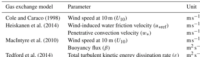
Table 1.Parameters used in the parameterizations of the gas transfer velocity in the gas exchange models by Cole and Caraco (1998), Heiskanen et al. (2014), MacIntyre et al. (2010), and Tedford et al. (2014).

Gas exchange model Parameter Unit

Cole and Caraco (1998) Wind speed at 10 m (U10) m s−1

Heiskanen et al. (2014) Wind-induced water friction velocity (u∗ref) m s−1

Penetrative convection velocity (w∗) m s−1

MacIntyre et al. (2010) Wind speed at 10 m (U10) m s−1

Buoyancy flux (β) m2s−3

Tedford et al. (2014) Total turbulent kinetic energy dissipation rate (ε) m2s−3

εs=u3∗w/κz

0_{, whereu}

∗wis the wind-induced water-side fric-tion velocity,κ=0.4 is the von Kármán constant, andz0 is a reference depth, and convective turbulence production εc, which equals the buoyancy fluxβas

εTE= (

0.56εs+0.77|εc| ifβ <0, 0.6εs ifβ≥0,

(7)

The wind-induced water friction velocityu∗wcan be calcu-lated from the atmospheric friction velocityu∗a=(τ/ρa)0.5, whereτ is the wind shear stress andρais the density of air, as in MacIntyre et al. (1995):

u∗w=u∗a ρ_a

ρw 0.5

. (8)

2.1.2 Gas exchange models

The widely applied experimental wind-based regression for-mula forkby Cole and Caraco (1998) gives the gas transfer velocity in (cm h−1) as

kCC=

2.07+0.215U₁₀1.7

Sc

600 −0.5

, (9)

whereU10 (m s−1) is the wind speed at 10 m andScis the temperature-dependent Schmidt number of CO2.

In the boundary-layer model by Heiskanen et al. (2014), the wind-induced water friction velocity is approximated to be a linear function of the wind speed at 1.5 m of height,U1.5:

u∗ref=C1U1.5, (10)

where C1 is an empirical dimensionless constant, and the equation forkHE(m s−1) is

kHE=

(C1U1.5)2+(C2w∗)2

0.5

Sc−0.5, (11) whereC1=1.5×10−4andC2=0.07 is another experimen-tal dimensionless constant. The model by Heiskanen et al. (2014) is used in the vertical process-based Arctic Lake Bio-geochemistry Model (ALBM) (Tan et al., 2017), which sim-ulates inorganic and organic carbon cycling in permafrost

lakes. The model by Heiskanen et al. (2014) is also included in the LakeMetabolizer package (Winslow et al., 2016), in which several lake metabolism models can be combined with models for computing the gas transfer velocity.

In the simple wind-based regression model by MacIntyre et al. (2010), the gas transfer velocitykMI(cm h−1) is calcu-lated separately for heating and cooling conditions as

kMI=   

 

(2.04U10+2.0)

Sc

600 −0.5

ifβ <0, (1.74U10−0.15)

Sc

600 −0.5

ifβ≥0.

(12)

In the surface renewal model of air–water gas exchange, kis parameterized as a function of the total turbulent kinetic energy dissipation rate ask=c(νε)0.25Sc−0.5, wherecis an empirical dimensionless constant andνis the kinematic vis-cosity of water (MacIntyre et al., 1995). Tedford et al. (2014) integrated the parameterization of the total turbulent kinetic energy dissipation rate,εTE, into the surface renewal model to yield a model for the gas transfer velocity in units of me-ters per second:

kTE=c(νεTE)0.25Sc−0.5. (13)

The models by Cole and Caraco (1998), Heiskanen et al. (2014), and Tedford et al. (2014) are included in a gas ex-change model intercomparison study by Dugan et al. (2016).

2.1.3 Lake model MyLake C

MyLake v1.2 (Saloranta and Andersen, 2007), which simu-lates lake thermal structure, seasonal ice and snow cover, and phosphorus–phytoplankton dynamics. In the model, vertical heat and mass diffusion are calculated with a diffusion equa-tion using a vertical turbulent diffusion coefficient derived from the buoyancy frequency and parameterized by lake sur-face area by default. Settling of particulate substances is also taken into account in the equation. In addition, convective and wind-induced water column mixing processes are in-cluded. As an exception to the daily time step, heat exchange between the water column and the atmosphere is calculated separately for daytime and nighttime. MyLake v1.2 and its various extensions have been used in studies on stratification and lake ice cover (e.g., Saloranta et al., 2009; Dibike et al., 2012; Gebre et al., 2014), total phosphorus concentration and phytoplankton biomass (e.g., Romarheim et al., 2015; Cou-ture et al., 2018), dissolved organic carbon (DOC) concen-tration (Holmberg et al., 2014; de Wit et al., 2018), and dis-solved oxygen (DO) conditions (Couture et al., 2015).

MyLake C has been designed to include only the most sub-stantial physical, chemical, and biological processes related to carbon cycling in a well-balanced and robust way. CO2 is produced in the lake through organic carbon degradation both within the water column as well as in the sediment and through phytoplankton respiration. Inorganic carbon produc-tion is coupled to DO consumpproduc-tion and vice versa. A di-vision is made between readily degradable, phytoplankton-originated autochthonous particulate organic carbon (POC) and more refractory allochthonous POC. The model also in-cludes the sedimentation, resuspension, and permanent burial of POC. Correspondingly, DOC is classified into three com-pound classes with different bacterial degradabilities. A sep-arate submodule (Holmberg et al., 2014) calculates the con-version of DOC into DIC via bacterial and photochemi-cal degradation. The meteorologiphotochemi-cal model forcing includes daily global radiation, cloud cover fraction, atmospheric tem-perature, relative humidity, atmospheric pressure, wind speed at 10 m of height, and precipitation. Hydrological forcing data include daily inflow volumes, inflow temperatures, in-flow pH, and the inin-flow concentrations of modeled sub-stances, including DOC, POC, and DIC. Complete data re-quirements are presented and model structure and applied equations are described in detail in Kiuru et al. (2018).

MyLake uses the Air–Sea Toolbox (Air-Sea, 1999) based on the parameterizations and algorithms in Fairall et al. (1996) for the calculation of surface wind stress and the com-ponents of surface heat flux. The sensible heat fluxQH, the latent heat fluxQL, and the wind shear stressτ are obtained

from aerodynamic bulk formulas of the form

QH=ρacpaChU (Ta−Ts), (14)

QL=ρaLeClU (qa−qs), (15)

τ =ρaCdU2, (16)

wherecpa is the specific heat capacity of air, ChandCl are

the transfer coefficients of sensible and latent heat, respec-tively,Cdis the drag coefficient,U is wind speed,Ta is air temperature, Ts is water surface temperature, Le is the la-tent heat of evaporation of water,qais the specific humidity, andqs is the saturation specific humidity at the water sur-face temperature. No wind-sheltering effect onU is applied in the calculation of surface wind stress and surface heat flux components.

The air–water CO2fluxFCO2 (MyLake C: mg m

−2_d−1₎ is calculated with Eq. (1) using the model forkby Cole and Caraco (1998) (Eq. 9). The chemical enhancement factorα is set to 1, and the temperature dependence of the aqueous-phase solubilityKHis calculated according to Weiss (1974). In this study, we incorporated the models forkby Heiska-nen et al. (2014) (Eq. 11), MacIntyre et al. (2010) (Eq. 12), and Tedford et al. (2014) (Eq. 13) into MyLake C as al-ternatives to the default model by Cole and Caraco (1998). The constants in the model by Tedford et al. (2014) are de-fined asc=0.5 andz0=0.15 m as in Erkkilä et al. (2018). In MyLake C, the actively mixing layer includes the model grid layers in which the water column temperature is within 0.02◦C of the temperature of the topmost grid layer. The temperature dependence ofScfor CO2is determined for sur-face water conditions using the polynomial fit in Wanninkhof (1992). The approximationU10/U1.5=1.22 is used for the wind speed at different heights.

2.2 Model application

We used the MyLake C application to Lake Kuivajärvi pre-sented in Kiuru et al. (2018) as the basis of the study. The model setup, including model forcing data and the initial in-lake conditions, is nearly identical to that described in Ki-uru et al. (2018). The minor differences are pointed out in Sect. 2.2.2.

2.2.1 Study lake

is 0.65 years. Lake Kuivajärvi is surrounded by managed mixed coniferous forest together with small open wetland ar-eas (Miettinen et al., 2015). The majority of the catchment area (9.4 km2) of the lake is flat. The main inlet stream with a mean pH of 6.5 (Dinsmore et al., 2013) drains four upstream lakes, which are smaller in area than Lake Kuivajärvi. The lake is dimictic: the spring turnover usually occurs rapidly right after ice-off in late April or early May, and the sum-mer stratification period lasts until the autumn turnover in September or October. The duration of the ice-covered pe-riod and the concomitant inverse stratification is usually 5– 6 months (Heiskanen et al., 2015). The turnover periods are hot moments for the release of CO2accumulated in the hy-polimnion of the lake during stratification (Miettinen et al., 2015). Because of high terrestrial inputs of organic matter, the median concentration of DOC in the surface water is 12– 14 mg L−1_{(Miettinen et al., 2015) and water clarity is rather} low, with a median light attenuation coefficient KL being around 0.6 m−1(Heiskanen et al., 2015).

2.2.2 Model forcing and calibration data

The meteorological forcing data and hydrological loading data used in the model application are described in detail in Kiuru et al. (2018). The daily averages of wind speed at 1.5 m and incoming shortwave radiation together with in-lake tem-perature and CO2 concentration were obtained from auto-matic platform measurements (Heiskanen et al., 2014; Mam-marella et al., 2015); the remaining meteorological forcing data were obtained from SMEAR II or from weather stations (Finnish Meteorological Institute) in Hyytiälä located less than 1 km from the lake (precipitation) and in Tikkakoski lo-cated approximately 95 km to the northeast of the lake (cloud cover fraction). Differing from Kiuru et al. (2018), the CO2 mixing ratio in the atmosphere was assumed to be 395 ppm on the basis of the rather fragmentary time series of high-frequency in situ measurements of the CO2mixing ratio, the method of which is described in Erkkilä et al. (2018).

The construction of the time series for lake inflow was based on continuous measurements of the discharges at the main inlet and at the outlet of Lake Kuivajärvi in 2013–2014 (Dinsmore et al., 2013). Because the total measured outflow volumes were approximately double the main inlet discharge volumes on an annual scale, the daily inflow volumes were corrected by a factor of 2 in order to include the potential contributions of smaller inlet streams and groundwater to lake inflow. At the main inlet, water temperature was mea-sured approximately two times a month in 2013 and con-tinuously in 2014, and CO2concentration was measured two times a month in 2013 but mostly at intervals of 2–3 d around the period of ice-off in April and May using the procedure described in Miettinen et al. (2015). Daily time series were generated by linear interpolation.

The model was calibrated against the daily averages of the automatic high-frequency CO2concentration measurements:

an optimal set of selected model parameters was estimated so that the simulated CO2concentration time series matched the corresponding measured CO2 concentration time series as well as possible. The estimation was performed using a sta-tistical inference algorithm. In addition, the automatic water column temperature measurements were used in model per-formance validation. The CO2concentrations were measured at 0.2, 1.5, 2.5, and 7.0 m, and the temperature measurements were performed at 0.2 m, at 0.5 m intervals from 0.5 to 5.0 m, and at 6, 7, 8, 10, and 12 m using the measurement systems described in Heiskanen et al. (2014) and Mammarella et al. (2015).

2.2.3 Model assessment data

The estimation of the flux footprint distribution functions was made using the model by Kormann and Meixner (2001). The average footprint contributing to 80 % of the fluxes varies from 100 up to about 300 m from the measurement platform depending on atmospheric stability conditions as described in Mammarella et al. (2015). Only wind directions along the lake (130–180 and 320–350◦) were included in the calculations to ensure that heat fluxes from the surrounding land were excluded. Furthermore, possible remaining effects of transversal advection during calm nights were removed through EC quality screening. In addition to the exclusion of some of the EC measurement data through the application of the quality screening criteria presented in Erkkilä et al. (2018), there was a gap in the heat flux data on 14–27 June because of EC system malfunction. The monthly data cover-age was 43 %–69 % and 32 %–70 % of the original data for sensible and latent heat fluxes, respectively. We constructed gap-filled half-hour time series for sensible and latent heat fluxes using linear fits between the measured sensible heat flux and wind speed multiplied by the air–surface water tem-perature difference and between the measured latent heat flux and wind speed multiplied by the vapor pressure difference, according to Mammarella et al. (2015). Only the vapor pres-sures calculated from the measured relative humidities were used in the latter fit. The fitting was performed independently for each month.

We compared the simulated gas transfer velocities for CO2 and the simulated air–water CO2fluxes to those determined directly from measurements using the corresponding gas ex-change models. The latter are hereinafter referred as to calcu-lated gas transfer velocities and calcucalcu-lated CO2fluxes. The calculated CO2 transfer velocities for each of the four gas exchange models were obtained using the daily averages of required measured variables. The calculated air–water CO2 fluxes were further obtained as the product of the calculated CO2 transfer velocities and the daily averages of the mea-sured air–water CO2concentration gradient. The conditions were thus compatible with the daily time step applied in My-Lake C. The atmospheric equilibrium concentrations of CO2 were calculated from the measured atmospheric CO2 mix-ing ratios. The daily averages of the depth of the AML were estimated from the daily averaged temperature profiles as the depth at which water column temperature was within 0.25◦C of the temperature at 0.2 m as in Erkkilä et al. (2018). As in MyLake C, the approximationU10/U1.5=1.22 was used in the calculations. Following Mammarella et al. (2015), a value of 2 m−1_{was used for the total attenuation coefficient} of shortwave radiationKLin the calculation ofQeff.

2.2.4 Model calibration and validation

We estimated the MyLake C parameters utilizing a Markov chain Monte Carlo-based Bayesian inference algorithm fol-lowing the procedures in the original calibration of the Lake Kuivajärvi application presented in Kiuru et al. (2018). Each

of the four new versions of the MyLake C Lake Kuiva-järvi application, using the models forkby Cole and Caraco (1998) (both the MyLake C version and the respective gas exchange model being hereinafter referred to as CC), Heiska-nen et al. (2014) (HE), MacIntyre et al. (2010) (MI), and Tedford et al. (2014) (TE), was calibrated individually. The simulations with the MyLake C versions using different gas exchange models are hereinafter collectively referred to as GEMs. The model grid length was 0.5 m. The model was run from 8 January 2013 to 31 December 2014. The calibration period extended from 8 January to 31 December 2013, and the measurements in 2014 were used for model validation.

The calibrations were performed against the daily averages of the automatic water column CO2concentration measure-ments at the depths of 0.2, 2.5, and 7 m. We chose to ap-ply the automatic measurements instead of the corresponding manual measurements used in the model calibration in Kiuru et al. (2018) because the calculation of daily CO2fluxes was based on the automatic measurements at 0.2 m in this study, and the simulation results were thus comparable with the cal-culated CO2fluxes. Even though the near-surface CO2 con-centration was the most significant factor considering air– water CO2 exchange, deeper depths were included so that model behavior would also remain reasonable at deeper lev-els.

The calibrated model parameters were selected on the ba-sis of the original calibration. However, because the new cal-ibrations were not performed against water column DO con-centrations, the parameters related to interactions between DO and CO2, the photosynthetic quotient and the respira-tory quotient, were excluded from the parameter set. The DIC inflow concentration scaling factorCDI,IN, applied dur-ing open-water seasons, was introduced as a new calibra-tion parameter. The other parameters included in the cali-bration were the vertical turbulent diffusion parameterak, the wind-sheltering coefficient Wstr, the DOC-related spe-cific attenuation coefficient of photosynthetically active radi-ationβDOC, the maximal phytoplankton growth rate at 20◦C µ0₂₀, the phytoplankton death rate at 20◦Cm20, the degrada-tion rates of labile DOCkDOC,1and semilabile DOCkDOC,2, the fragmentation rates of autochthonous POCkPOC,1 and allochthonous POCkPOC,2, and the sedimentary POC degra-dation ratekPOC,sed. The parameters obtained in the original calibration, or the default parameters, were used as the means of the prior parameter distributions.

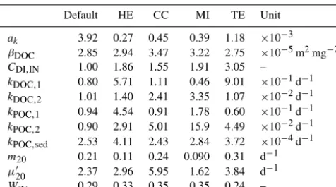
Table 2.Calibrated model parameters for the different versions of MyLake C application to Lake Kuivajärvi with different incorpo-rated gas exchange models (HE: Heiskanen et al., 2014, CC: Cole and Caraco, 1998, MI: MacIntyre et al., 2010, TE: Tedford et al., 2014). The default parameter values were used as the means of the prior parameter distributions.

Default HE CC MI TE Unit a_k 3.92 0.27 0.45 0.39 1.18 ×10−3 β_DOC 2.85 2.94 3.47 3.22 2.75 ×10−5m2mg−2 CDI,IN 1.00 1.86 1.55 1.91 3.05 –

k_DOC,1 0.80 5.71 1.11 0.46 9.01 ×10−1d−1 kDOC,2 1.01 1.40 2.41 3.35 1.07 ×10−2d−1 k_POC,1 0.94 4.54 0.91 1.78 0.60 ×10−1d−1 k_POC,2 0.90 2.91 5.01 15.9 4.49 ×10−2d−1 kPOC,sed 2.53 4.11 2.43 2.84 3.72 ×10−4d−1 m₂₀ 0.21 0.11 0.24 0.090 0.31 d−1 µ0₂₀ 2.37 2.96 5.95 1.62 3.84 d−1

Wstr 0.29 0.33 0.35 0.35 0.24 –

gives a relative evaluation assessment, determining the rela-tive magnitude of the residual variance compared to the vari-ance of measurement data (Moriasi et al., 2007). The value of the normalized bias (B∗) describes a systematic overesti-mation (B∗>0) or underestimation (B∗<0) of a state vari-able in the simulation, whereas the normalized unbiased root mean square difference (RMSD0∗) shows if the standard de-viation of the simulated values is higher (RMSD0∗>0) or smaller (RMSD0∗<0) than that of the measurements (Los and Blaas, 2010).

2.2.5 Calculation of CO2budgets

After the calibrations, we calculated CO2 budgets for the epilimnion of the lake during periods of continuous sum-mer stratification in 2013 and 2014 for each GEM. The epil-imnion was defined as the layer in which water temperature was within 1◦C of surface temperature. The stratified period was defined to begin on the day of the formation of the ther-mocline after ice-off and to finish when the depth of the epil-imnion (zepi) reached the value of 7 m in the simulations. The exchange of CO2between the epilimnion and the atmosphere is balanced in MyLake C by (1) net external loading of CO2, (2) net epilimnetic CO2 production, and (3) the release of CO2from deeper layers to the epilimnion. The net external loading equals the amount of terrestrially produced CO2 en-tering the lake via stream inflow subtracted by the amount of CO2in lake outflow. The release of CO2from the metal-imnion or the hypolmetal-imnion occurs through the deepening of the epilimnion due to wind-induced mixing or thermal con-vection. If the epilimnetic volume becomes smaller, a por-tion of CO2is again confined below the epilimnion and the amount of CO2in the remaining epilimnion is reduced.

3 Results

3.1 Model calibration

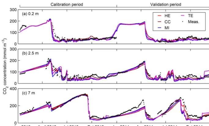
Even though the differences between the formulations of the gas exchange models incorporated into MyLake C are rather notable, the resultant CO2concentrations did not differ sub-stantially between the GEMs, that is, between the simula-tions with the MyLake C versions using different gas ex-change models (Fig. 1). However, an optimal simulation re-sult can be attained through many different combinations of processes related to in-lake carbon dynamics and fluvial and atmospheric exchange in MyLake C, which is seen in the variation between the parameter values obtained from the different calibrations (Table 2). The calibrations were per-formed only against CO2concentrations, and the aim of the calibration was not to try to reproduce the actual in-lake car-bon cycling but rather to compare different possible ways to generate an optimal water column CO2concentration. The performance metrics for CO2 concentration shown in the Supplement (Table S1) indicate that all GEMs yielded CO2 concentrations (B∗<0) that were too low at all depths dur-ing the calibration and validation periods with only a few exceptions. However, the CO2concentration measurements performed during the ice-covered periods were largely not applicable at 0.2 m because of the lake ice cover and some-times also inapplicable at deeper levels because of incorrect functioning of the measurement system.

The average near-surface (0–0.5 m) CO2 concentrations over the open-water seasons were notably higher in CC (44.3 and 40.3 mmol m−3 in the calibration year 2013 and in the validation year 2014, respectively) than in the other GEMs (HE: 34.2 and 31.6 mmol m−3_{; MI: 31.5 and 29.4 mmol m}−3_; TE: 36.9 and 34.1 mmol m−3). Only the days with avail-able corresponding water column CO2 concentration mea-surement data were included in the averaging of the simu-lated near-surface CO2 concentrations over the open-water seasons. By contrast, the averages of the measured near-surface (0.2 m) CO2concentrations over the open-water sea-sons were 45.2 mmol m−3 in 2013 and 37.2 mmol m−3 in 2014. Thus, CC yielded a higher near-surface CO2 concen-tration compared to the measurements in 2014 when only the ice-free season, the period of air–water CO2 exchange, is considered. The simulated open-water seasons were deter-mined from the simulated ice-off and ice-on dates. Because CO2 flux differs from zero starting from the day after ice-off in MyLake C, the simulated open-water seasons applied in the study were 3 May–25 November 2013 and 16 April– 22 November 2014. In 2013, the observed open-water season lasted from 1 May to 27 November. In 2014, the observed ice-off date was 12 April.

calibra-Figure 1.Simulation results for CO₂concentration with each GEM (mmol m−3) versus the daily averages of automatic high-frequency CO₂ concentration measurements at the depths of(a)0.2 m,(b)2.5 m, and(c)7.0 m in Lake Kuivajärvi during the calibration year 2013 and the validation year 2014.

tion period and the validation period, respectively; HE: 5.44 and 5.33 cm s−1; MI: 5.87 and 5.82 cm s−1; TE: 4.73 and 4.66 cm s−1). The differences in the simulated fluxes between GEMs were dissimilar to those in k because of the differ-ences in the simulated near-surface CO2concentrations. The smallestkvalues in CC were compensated for by the highest near-surface CO2 concentrations. By contrast, a high daily CO2efflux due to a highkin MI reduced the simulated near-surface CO2concentration compared to the other GEMs dur-ing the whole simulation period. Overall, the differences in yearly air–water CO2 fluxes between GEMs were smaller than those in the values ofk(CC: 0.22 and 0.20 µmol m−2s−1 for the calibration period and the validation period, re-spectively; HE: 0.28 and 0.26 µmol m−2s−1; MI: 0.25 and 0.24 µmol m−2s−1; TE: 0.28 and 0.27 µmol m−2s−1).

The CO2efflux during the first few days after ice-off was higher in GEMs with a high k, which increased the water column pH in comparison to CC. The differences remained rather constant during most of the open-water seasons. The near-surface pH was on average 0.20–0.26 and 0.18–0.25 units higher in the other GEMs than in CC during the open-water seasons of 2013 and 2014, respectively. As a result, the average fractions of CO2of DIC in the near-surface layer were respectively 6–8 and 5–6 percentage units higher in CC than in other GEMs, which also contributed to the higher near-surface CO2concentration in CC than in other GEMs. In addition, the open-water season average near-surface pH was 0.22 units higher in 2014 than in 2013 in all GEMs. Ac-cumulation of bicarbonate in the water column in the course of the simulations may have resulted in an excessively high pH and thus a relatively lower CO2 concentration in 2014 compared to 2013.

The differences in simulated temperatures between GEMs, primarily due to different attenuation of shortwave radiation in the water column, were rather small, especially at 0.2 m and at 2.5 m (Fig. S6). High epilimnetic concentrations of both Chl a and DOC, resulting from a low phytoplankton death rate and a high allochthonous POC fragmentation rate, respectively, in MI resulted in the strongest attenuation of shortwave radiation and thus the highest near-surface tem-perature because of a thinner and warmer epilimnion than in other GEMs. The open-water season average near-surface temperatures were 0.28–0.47 and 0.65–0.86◦C lower than the corresponding measured averages in the calibration and validation periods, respectively, being highest in MI and low-est in TE. The differences were greatlow-est in November before ice-on. The simulated near-surface temperatures tended to be somewhat too low in spring and early summer during both periods and somewhat too high in the late summer and au-tumn of the calibration year.

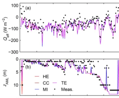
Figure 2. (a)Daily effective surface heat fluxes (W m−2) simulated with each GEM and calculated on the basis of heat flux measure-ments.(b)Simulated and empirically determined depths of the daily actively mixing layer (m) in Lake Kuivajärvi in May–October 2013.

deepening was slowest in HE because a somewhat stronger temperature gradient in the metalimnion, which was due to the smallestak, and resisted wind-induced thermocline ero-sion during summer.

3.2 Effective heat flux

The effective heat fluxes at the air–water interface simulated with each GEM on 3 May to 31 October 2013 and the corre-sponding values calculated on the basis of heat flux and radi-ation measurements are presented in Fig. 2a. The largest dif-ferences between the magnitudes and the directions of simu-lated and measuredQeffwere seen in early May. The simu-latedQeffwas directed out of the lake throughout the study period except for a few occasions in early May and in Octo-ber, whereas measurement-based calculations yielded more frequent occurrences of a positive dailyQeff. Also, a nega-tiveQeffwas often overestimated by the simulations because of overly high negative sensible and latent heat fluxes and net longwave radiation (Fig. S7). The performance of the simu-lation of the components of surface heat flux was rather poor (Table S2). Overall, the Qeff simulation performance was not very good (R2=0.39–0.41, RMSE=48.2–49.2 W m−2, NS=0.11–0.14,B∗= −0.47. . .−0.46,n=164). The differ-ences in the simulatedQeffbetween GEMs, resulting mainly from different surface temperatures, were quite small.

The extent of shortwave radiative heating of the AML, QSW,AML, is dependent onzAML. The simulatedzAML was greater than the measured daily average with a few excep-tions at the beginning and near the end of the study period (Fig. 2b), which increased the simulated QSW,AML and de-creased a negative Qeff. The simulation with a daily time step generated clear temperature variation in the epilimnion only on days with a high amount of surface heating in early summer and midsummer, which resulted in an overly deep

AML during most of the period. In addition, the model with a sequential description of thermal processes did not catch simultaneous wind mixing and surface heat exchange pro-cesses that resulted in a deeper observational AML in spring and late autumn. However, day-to-day variation in the dis-crepancy of QSW,AML was high throughout the study pe-riod. Also, the simulations highly underestimated the at-mospheric friction velocity (R2=0.35, RMSE=0.11 m s−1, NS= −3.2,B∗= −1.89,n=166) (Fig. S8), the simulated u∗a being on average only 46 % of the measured daily av-erage. The simulated daily drag coefficientCdat 1.5 m was affected by atmospheric stability conditions. The medianCd varied from 1.589×10−3to 1.593×10−3between the GEMs.

3.3 CO2exchange

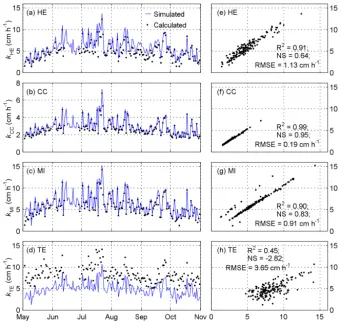
The differences between simulated gas transfer velocities for CO2 and the respective calculated values during the study period 3 May–31 October 2013 were rather small in the cases of gas exchange models based solely on wind speed, CC and MI, but the discrepancies were higher in HE and TE, which also include the effect of thermal convection on gas exchange (Fig. 3, Table S3). The simulations with CC and MI often yielded slightly higher values ofkthan the re-spective calculations because the simulated surface tempera-ture was higher than the measured daily average (Fig. S6), and thus the temperature-dependent Schmidt number cor-rection of k was different. Also, the occurrences of a sim-ulated negative β in early May in MI yielded higher kMI compared to the respective calculated values obtained from the observed positiveβ. The simulatedkHEwas often higher than the calculated counterpart because of a high negative Qeff or a deep AML in the simulations (Fig. 2), which re-sulted in a high penetrative convection velocity. In HE, the effects of wind-induced shear and thermal convection onk are set to be roughly of the same order of magnitude and the wind-induced shear velocity is calculated from wind speed, whereas CO2flux is driven principally by wind shear, which is calculated directly fromu∗a, in TE. Because the simulated u∗awas consistently significantly lower than the correspond-ing daily measured average, the simulatedkTEwas on aver-age 40 % lower than the calculated value.

Figure 3.Simulated and calculated gas transfer velocities for CO2(cm h−1) in Lake Kuivajärvi on 3 May–31 October 2013 obtained with

the gas exchange models by(a, e)Heiskanen et al. (2014),(b, f)Cole and Caraco (1998),(c, g)MacIntyre et al. (2010), and(d, h)Tedford et al. (2014).

gradients in May resulted in an underestimated air–water CO2 flux from the water column compared to the respec-tive calculated fluxes (Fig. 5, Table S3). The simulated flux was notably lower than the calculated flux in TE during the whole study period because of a smallkTE. In contrast, CC notably overestimated the corresponding calculated CO2flux in August and September because of a high simulated near-surface CO2concentration. Also, the simulated CO2flux was slightly higher than the calculated flux in HE in August and September because of high epilimnetic net CO2production. The total simulated CO2flux during May–October matched the calculated flux in CC but was notably lower in HE and MI and less than half of the calculated flux in TE (Table 3). The underestimated near-surface CO2concentrations were some-what compensated for by the higher simulatedkHEandkMI compared to the calculated counterparts, which decreased the difference between the simulated and calculated fluxes in HE and MI.

The applied gas exchange models yielded notably different calculated monthly CO2effluxes (Table 3). The CO2fluxes were calculated using the measured air–water CO2 concen-tration gradients, and thus the differences between the

calcu-Table 3.Total and monthly averages of simulated and calculated CO2 fluxes (µmol m−2s−1) in May–October 2013 obtained with

different gas exchange models. Only the days with available mea-surement data are included in the averaging of the simulated fluxes. Monthly values for June are excluded because measurement data were available only for 7 d.

May–October May July Calc. Sim. Calc. Sim. Calc. Sim. Heiskanen 0.38 0.31 0.79 0.41 0.37 0.34 Cole and Caraco 0.23 0.24 0.53 0.33 0.20 0.26 MacIntyre 0.45 0.29 0.97 0.52 0.44 0.26 Tedford 0.71 0.30 1.90 0.43 0.56 0.33

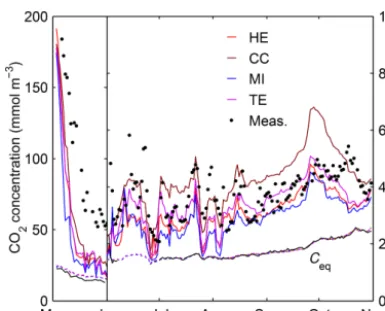
Figure 4.Simulated CO2concentrations (mmol m−3) in the surface

layer (0–0.5 m) obtained with each GEM and the daily averages of the automatic measurements at 0.2 m in Lake Kuivajärvi in May– October 2013. Also shown are the atmospheric equilibrium concen-trations of CO2(Ceq) obtained from the simulations (dotted colored

lines) and calculated from the measured atmospheric CO2

concen-tration and surface water temperature (solid black line). Note the different vertical scales in May and in June–October.

lated fluxes were only due to different values ofk. Monthly fluxes calculated with MI were nearly or even more than dou-ble those calculated with the other wind-based model CC. Days with a positive β, resulting in a lower kMI, occurred mainly in May and October, and thus the difference be-tween the CO2fluxes calculated with MI and CC was slightly smaller in those months. The models that include the effect of thermal convection, HE and TE, yielded notably higher CO2 fluxes than the simplest model, CC. Nevertheless, the CO2 fluxes calculated with MI were slightly higher than those cal-culated with HE. The CO2 fluxes calculated with TE were clearly the highest in all months, which was, however, not the case in the simulations.

The calculated daily values of k and CO2 flux were dependent on the calculation interval. If the daily k had been calculated as the daily average of calculated half-hour values of kinstead of using the daily averages of the input variables, the results would have been different. The daily averages of calculated half-hourkMI(RMSE=0.70 cm h−1, B∗= −0.16) andkTE (RMSE=0.22 cm h−1, B∗= −0.04) were lower than the respective values calculated using daily averages of input variables, whereas the opposite was the case for kHE (RMSE=0.48 cm h−1, B∗=0.20) and kCC (RMSE=0.16 cm h−1, B∗=0.15). In con-trast, the calculation of a daily CO2 flux as the aver-age of half-hour fluxes yielded a slightly higher CO2 flux in all GEMs (HE: RMSE=0.066 µmol m−2s−1, B∗=0.13; CC: RMSE=0.034 µmol m−2s−1, B∗=0.11; MI: RMSE=0.10 µmol m−2s−1,B∗=3.4×10−4; TE: RMSE=0.11 µmol m−2s−1,B∗=0.05).

The differences resulting from the different methods of the calculation of a dailykcan partly be explained by the

behav-ior of the driving variables of the models. Using the daily averages of the input variables in the calculation may have smoothened out the effects of the spells of stronger nega-tive buoyancy flux or a deeper AML that increase the half-hourkHE and the effects of the occasions of positive buoy-ancy flux that decrease the half-hourkMI. Daily averaging of wind speed may have cut out the rapid increase inkCC un-der stronger wind conditions during the course of day due to the greater-than-linear dependence ofkCCon wind speed. By contrast, because the dependence ofkTEonu∗a is less than linear and the impact of thermal convection onkTEis minor, the effect of the diel variation ofu∗aand thus the relative dif-ference between the methods of the calculation ofkTE was rather small.

3.4 Lake CO2budgets

The simulated CO2 budgets for the epilimnion of the lake during periods of continuous summer stratification in 2013 and 2014 differed between GEMs as a response to different CO2effluxes (Table 4). The simulations were not able to re-produce the short-lived episodes of a very shallow epilimnion on days with high solar radiation and low wind speeds in late August and early September 2013, but at other times the simulatedzepi matched the depths estimated from the mea-sured daily temperature profiles rather well (Fig. 6). The epil-imnion formed 11 d earlier and extended to 7 m 16–22 d later in 2013 than in 2014. The in-lake CO2concentrations were higher at the onset of stratification in 2013 than in 2014 be-cause of less effective water column ventilation during the shorter spring mixing period. As a result, the amount of CO2 in the epilimnion decreased during the stratified period in 2013, whereas it increased slightly in 2014.

Figure 5.Simulated and calculated air–water CO2fluxes (µmol m−2s−1) in Lake Kuivajärvi on 3 May–31 October 2013 obtained with the

gas exchange models by(a, e)Heiskanen et al. (2014),(b, f)Cole and Caraco (1998),(c, g)MacIntyre et al. (2010), and(d, h)Tedford et al. (2014).

Figure 6.Simulated and observed depths of the epilimnion (m) in Lake Kuivajärvi during the continuous summer stratification in 2013 and 2014. The simulations were performed using each of the gas exchange models incorporated into MyLake C.

However, a high phytoplankton biomass did not imply high CO2consumption because of phosphorus limitation of phytoplankton growth in the model and the resultant reduc-tion of photosynthetic CO2 consumption under high Chla and low bioavailable phosphorus concentrations in the sim-ulations. Instead, CO2fixation occurred at a steady rate and the total CO2consumption over the whole growing season was relatively higher under a low Chlaconcentration due to a highm. The highest average phytoplankton biomass in HE

resulted in the highest CO2fixation; however, total net CO2 production was also highest in HE because of highkPOC,1 andkDOC,1. Small values ofkPOC,1andkDOC,2resulted in a relatively low net CO2production despite low CO2fixation and a highkPOC,sedin TE. Net CO2production was lowest in CC because of rather high total CO2fixation during the long growing season and the rather smallkPOC,1andkDOC,1.

Table 4.Simulated CO₂budgets (kg CO₂) for the epilimnion of Lake Kuivajärvi during summer stratification in 2013 and 2014 using different gas exchange models incorporated into MyLake C.

Heiskanen Cole and Caraco MacIntyre Tedford

2013

Net production 52 300 38 700 40 400 44 800

Change due to efflux∗ −89 900 −72 300 −74 500 −89 200

Net external loading 10 800 8600 11 000 18 500

Change due to epilimnion deepening 16 100 15 100 15 800 18 800

Change in epilimnetic storage −10 700 −9900 −7200 −7100

Duration (d) 134 134 134 134

2014

Net production 38 300 24 900 25 400 28 700

Change due to efflux∗ −63 600 −42 700 −46 600 −57 100

Net external loading 8300 6300 8100 12 200

Change due to epilimnion deepening 17 500 13 100 14 100 17 400

Change in epilimnetic storage 500 1600 1000 1200

Duration (d) 107 101 101 101

∗_{The change in water column CO}

2content due to CO2efflux was approximately 1 % lower than the amount of CO2evaded because of consequent equilibrium reactions in the carbonate system.

significantly increase the terrestrial CO2 input to the lake in GEMs with a high CO2 efflux. The measured inflow CO2concentration was 200–250 mmol m−3until ice-off, less than 80 mmol m−3during May, and mainly between 50 and 100 mmol m−3 during the summer and autumn. Thus, the default inflow CO2 concentration was only approximately double the simulated near-surface CO2concentrations during most of the open-water season, and the effect of external CO2 loading on in-lake CO2concentration was inevitably rather small, especially during the low-discharge period in late sum-mer and autumn. The values ofCDI,INdetermined the order of the amounts of the net external CO2load to the lake in the GEMs (TE: 42 000 and 45 000 kg CO2 over the years 2013 and 2014, respectively; MI: 27 500 and 31 400 kg CO2; HE: 26 500 and 30 600 kg CO2; CC: 22 200 and 25 800 kg CO2).

However, the total net external CO2loads to the lake over the stratification periods were slightly higher than the net ex-ternal CO2loads to the epilimnion in Table 4 because stream inflow was directed into the metalimnion on days when the inflow temperature was lower than the epilimnetic tempera-ture. The epilimnetic loads were 90 %–92 % and 98 %–99 % of the total loads in 2013 and 2014, respectively, the pro-portions being highest in CC and lowest in MI. The amount of CO2 outflow was relatively large in CC because of the high epilimnetic CO2 concentration; thus, the net external CO2 load was relatively lower in CC than in other GEMs compared to the differences in CDI,IN. In addition, because inflow pH was unaltered in the scaling of inflow DIC con-centration, some of the increased CO2 load was eventually evaded to the atmosphere in the simulations, but the bicar-bonate fraction of DIC remained in the water column, which resulted in a slight increase in in-lake pH and a decline in

the CO2fraction of DIC, especially in GEMs with a highk. Nevertheless, the impact of different amounts of bicarbonate loading on the in-lake pH was minor compared to the impact of different springtime CO2effluxes between GEMs.

4 Discussion

4.1 Differences between calculated and simulated CO2 fluxes

which is disadvantageous in a year-round, vertically layered lake model.

The day-to-day performance of the simulation of epilim-netic CO2 concentration was also partly determined by the simulated thermal stratification and epilimnetic volume. The simulations generally yielded a near-surface CO2 concentra-tion that was too low when the simulated zepi was in ac-cordance with the observed depth and performed more ad-equately only during periods when the simulated zepi was too high (Figs. 4 and 6). The measurements showed an in-crease in the near-surface CO2concentration when the epil-imnion became thicker, and vice versa, during the stratified period in 2013. Thermocline tilting-induced upwelling and convection-induced entrainment transported more CO2-rich water into the epilimnion on windy and cool days (Heiskanen et al., 2014). Conversely, high solar radiation input combined with calm conditions results in the warming of near-surface water and the formation of a thin epilimnion with a lower CO2concentration. High solar radiation also enhances pho-tosynthesis and thus increases the uptake of CO2(Provenzale et al., 2018). An overly deep simulated epilimnion resulted in enhanced CO2release from deeper layers and a higher total net CO2 production in a larger epilimnetic volume, which were able to compensate for the CO2 efflux in the simula-tions.

The accuracy of the determination of a dailyQeffand the applicability of the concept of a daily AML are issues that may cause uncertainties when gas exchange models are used either to calculate or to simulate daily estimates of k. The calculated half-hourQeffwas generally directed into the lake on some occasions during daytime because of solar heating of the AML and always directed out of the lake at night-time;zAML often increased during nighttime and decreased under the radiative heating of near-surface water during day-time. Boundary-layer models and surface renewal models have been developed to describe the short-term dynamics of turbulence in a shallow AML, and thus they may not perform equally well in calculations with a daily time step.

The wind-based CC yielded the lowest and the surface re-newal model TE the highest calculated air–water CO2fluxes, which is in line with the comparisons of different gas ex-change models using data from Lake Kuivajärvi by Mam-marella et al. (2015) and Erkkilä et al. (2018); however, the differences in simulated CO2 fluxes between CC and other GEMs were notably smaller than the corresponding differ-ences in the two experimental studies. The performance of TE is strongly dependent on the magnitude ofu∗a because wind shear is highly dominant over thermal convection as the generator of turbulence in the model. Because the simu-lations yielded significantly loweru∗a compared to the val-ues obtained through EC measurements (Fig. S8), the CO2 flux obtained with TE was much lower than the correspond-ing calculated flux. Also, Erkkilä et al. (2018) found that u∗a calculated from wind speed was lower than the mea-suredu∗ain Lake Kuivajärvi. Bulk models for surface stress

may yield low values foru∗aover a lake, especially when pa-rameterized for open-sea conditions with low surface rough-ness (Wang et al., 2015), which is the case in MyLake C. Lake size may also affect the relative differences between gas transfer velocities obtained with different gas exchange models. Dugan et al. (2016) applied different gas exchange models to the calculation of DO exchange in temperate lakes of various sizes. Simple, wind-based models yielded clearly lower values ofkthan more complex models in lakes sim-ilar to Lake Kuivajärvi in size, whereas the differences be-tween the model types were smaller in larger lakes with gen-erally higher wind speeds and a higher relative importance of wind-induced mixing compared to convection. In addition, ecosystem-specific empirical regression models may not be suitable for lakes with dissimilar characteristics (Vachon and Prairie, 2013).

4.2 Comparison to EC CO2flux measurements

Estimates of air–water CO2fluxes obtained with the gas ex-change models applied in our study have been compared with 30 min block-averaged EC CO2flux measurements over Lake Kuivajärvi (Heiskanen et al., 2014; Mammarella et al., 2015; Erkkilä et al., 2018). Heiskanen et al. (2014) com-pared the half-hourkcalculated with HE, CC, and MI with those obtained through EC measurements of CO2 flux in August–November 2011. In the study, the average values of kHE andkMI were approximately 70 % of the correspond-ing measurement-based values, but the averagekCCwas only about half of the averagekHE andkMI. Erkkilä et al. (2018) compared the daily medians of EC CO2flux during a 2-week period in October 2014 with the daily median CO2fluxes cal-culated with CC, HE, and TE. The CO2fluxes obtained with HE and TE were 60 % of the EC CO2 fluxes and approx-imately double the CO2 fluxes obtained with CC. Overall, TE yielded the best correspondence with the EC fluxes. TE also outperformed CC in the comparison of half-hour CO2 fluxes during the open-water periods of 2010 and 2011 in Mammarella et al. (2015). In our study, the best agreement with simulated and calculated CO2fluxes was found in CC, whereas TE yielded the lowest simulated fluxes in compari-son to the corresponding calculated fluxes. Thus, none of the GEM outputs can be considered compatible with EC CO2 fluxes, provided that the conclusions from the half-hour com-parisons in the abovementioned studies can be extended to a daily scale.

day because of the temporal bias of the measurements. EC flux measurements often tend to be inapplicable, especially at nighttime, because of flux nonstationarity during light winds and cooling (Heiskanen et al., 2014) or the advection of CO2 from the surrounding forest (Erkkilä et al., 2018). EC CO2 fluxes over boreal lakes are often enhanced at night by water-side convection (Podgrajsek et al., 2015) or because of a higher air–water CO2 concentration gradient due to the ab-sence of photosynthesis as a CO2sink (Erkkilä et al., 2018). Both the calculated and the simulated values ofkwere de-termined by means of the platform data. They were thus suit-able for comparison with each other but may not represent the average conditions over the lake and hence may not yield correct estimates of whole-lake CO2fluxes. Wind speed,u∗a,

QH, and QL were measured at a single point on the plat-form, and the source area of the EC measurements of u∗a,

QH, andQLranges from 100 to 300 m along the wind direc-tion over the lake (Mammarella et al., 2015). Thus, the values may not be representative for the whole lake. Wind speed and the resulting u∗a over lakes surrounded by forests are lower in sheltered nearshore areas than in the central zones of the lakes (Markfort et al., 2010). Sheltering affects the spa-tial variation of wind speed, especially in small lakes such as Lake Kuivajärvi. BecauseQH andQLare dependent on wind speed over the lake, they may also be higher at the cen-ter of the lake than in nearshore areas. Also, the estimation of u∗a,QH, andQL in the simulations was based on wind speed and other forcing data obtained from the single-point measurements, and the simulated values may have been over-estimates of the spatial averages. However, despite the same measurement location, some disparities existed between the simulated and measuredQHandQL. The differences may be in part attributed to an underestimation of surface heat fluxes by the EC method, which was seen, for example, in a study on energy balance over a small boreal lake by Nordbo et al. (2011) and also in Mammarella et al. (2015). The sum of the measured EC heat fluxes in Lake Kuivajärvi was on av-erage 83 % and 79 % of available energy in 2010 and 2011, respectively, in Mammarella et al. (2015). In addition, the total relative random error of the EC measurements is gener-ally around 10 % for both sensible heat flux and latent heat flux as estimated in Mammarella et al. (2015). Considerable spatial variability may also occur in near-surface water CO2 concentration in small, shallow boreal lakes (Natchimuthu et al., 2017), which may result in further discrepancies in the estimates on whole-lake CO2flux obtained on the basis of gas exchange models or by using a vertical, horizontally in-tegrated lake model.

4.3 Factors influencing the epilimnetic CO2budget

The model parameter sets obtained through calibration of the MyLake C applications using different incorporated gas ex-change models were notably different from each other, thus emphasizing different processes related to carbon cycling

within the water column or to carbon exchange with the sur-rounding terrestrial ecosystem or the atmosphere. However, considering the main objective of the study, which is the simulation of near-surface CO2concentration and air–water CO2flux, the different outcomes of the calibration processes, that is, the different model parameter sets, can be considered equally justified as they give insight on the diversity of bio-geochemical processes that impact lacustrine CO2dynamics. Phytoplankton is a significant factor in the lake CO2 bud-get and the main driver of the diurnal variation of CO2 con-centration in Lake Kuivajärvi (Provenzale et al., 2018). In MyLake C, inorganic carbon is fixed by phytoplankton and carbon is stored in autochthonous organic matter within the water column or in bottom sediments until it is mineralized by bacteria. A relatively large portion of epilimnetic phyto-plankton and dead autochthonous particulate organic matter sank from the epilimnion into deeper layers in MI because of the small values ofmandkPOC,1. Production of CO2via the degradation of phytoplankton-originated organic matter, as well as the release of bioavailable phosphorus in the epil-imnion through the mineralization of autochthonous organic matter, was also slow in MI because of a smallkDOC,1. As a result, the net production of CO2 in the epilimnion was rather low in MI (Table 4) despite the relatively high simu-lated phytoplankton biomass. Overall, differences in total net CO2consumption by phytoplankton during the stratified pe-riod between GEMs were rather small despite the large vari-ation in the simulated phytoplankton biomasses because of the phosphorus limitation of photosynthesis in GEMs with a high phytoplankton biomass and because of the variation in the length of the active growing season between GEMs.

The simulated Chlaconcentrations were rather constant over the growing season with the exception of the substan-tial spring growth peaks in CC and TE. There are no data on Chlaconcentration in Lake Kuivajärvi in 2013, but the Chla concentration at 0–3 m was at its highest, 30–50 mg m−3, in mid-July and decreased to a level of less than 2 mg m−3in late autumn in the years 2011–2012 (Heiskanen et al., 2015). The epilimnetic Chlaconcentration is usually 3–5 mg m−3 during the growing season with diatom-induced peaks un-der cool conditions in spring and autumn (Provenzale et al., 2018). Thus, the GEMs with low near-surface Chla concen-trations, CC and TE, may have yielded better estimates of the overall phytoplankton biomass than HE and MI. However, the net consumption of CO2by phytoplankton was not only related to the amount of phytoplankton biomass. Neverthe-less, none of the GEMs captured the supposed monthly varia-tion of epilimnetic CO2concentration caused by the seasonal succession of phytoplankton.

However, the use ofCDI,INcan be thought as the inclusion of the input of CO2through groundwater seepage to the lake. In budget calculations, groundwater DIC load can be generally estimated by applying groundwater DIC flow as a percent-age of stream DIC load (Chmiel et al., 2016). The amount of inflowing groundwater and its properties in Lake Kuivajärvi are unknown. However, in addition to inflow through minor inlet streams and surface runoff, especially during snowmelt in spring, groundwater seepage may contribute somewhat to the total lake inflow volume because the measured total out-flow volume over the year 2013 was approximately double the inflowing volume via the main inlet stream. The CO2 concentration in groundwater in southern Finland is around 700–900 mmol m−3(Lahermo et al., 1990), which is about tenfold higher than the estimated average inflow CO2 con-centration in Lake Kuivajärvi over the stratified period in 2013, 86 mmol m−3_{, and well in line with the yearly average} groundwater CO2 concentration near a boreal stream deter-mined by Leith et al. (2015). Thus, groundwater-derived CO2 transport to the lake may also affect the water column CO2 concentration.

The effect of CO2inputs through minor inlets or ground-water may be supported by the fact that the simulated near-surface CO2 concentration decreased too fast in all GEMs after ice-off in May 2013, that is, during a period when the snowmelt-induced flow in minor inlet streams may be sub-stantial and when the groundwater level is generally rela-tively high (Fig. 4). The simulated epilimnetic CO2 sinks were rather small at that time because net CO2consumption by phytoplankton was low in cool water and because CO2 ef-flux was relatively low because of a low air–water CO2 con-centration gradient. Labile, autochthonous DOC was absent in the epilimnion in the simulations, and the degradation of allochthonous DOC was slow under the relatively cold con-ditions in May. Despite the measured inflow CO2 concen-tration being approximately twice the simulated epilimnetic CO2concentration and the scaled inflow CO2concentrations and terrestrial CO2loads being even higher, the decline of the epilimnetic CO2 concentration was rapid in all GEMs. The high abundance of diatoms in Lake Kuivajärvi in spring may have resulted in a supply of easily degradable organic mat-ter, but net primary production also consumed CO2. Thus, substantial CO2loadings through surface runoff, minor inlet streams, or groundwater seepage could have been plausible additional sources of epilimnetic CO2in May, provided that the additional surface inflow was rich in CO2. The impact of groundwater seepage is supported by a study on the car-bon budget of a small boreal lake by Chmiel et al. (2016), in which a discrepancy between estimates of the gain and loss of inorganic carbon was explained by a possible underesti-mation of the impact of groundwater inflow.

4.4 Implications for lake modeling

None of the four MyLake C versions with different gas ex-change models surpassed the other ones in the study because of the complex interplay between the near-surface water CO2 concentration and air–water CO2flux in the simulations. A higher CO2efflux would have required a higher gain of CO2 in the lake through in-lake CO2production or external load-ing of inorganic carbon, but the MyLake C versions with gas exchange models yielding a highkwere not capable of in-creasing the CO2 gain sufficiently. Hence, it is not a triv-ial task to judge which of the four gas exchange models is most suitable for integration into MyLake C or other cou-pled physical–biogeochemical lake models. However, sev-eral experimental studies (e.g., Jonsson et al., 2008; Mac-Intyre et al., 2010; Heiskanen et al., 2014) have shown that traditional, wind-based models often yield low CO2 fluxes when compared to estimates based on direct measurements. Thus, it is recommended to strive to use the more sophisti-cated and probably more correct gas exchange models pro-vided that the biogeochemical lake model can be made adapt-able to higher CO2losses and that the parameters included in the more complex, turbulence-based models can be correctly simulated. This also means that further improvements related to the description of in-lake carbon processes in lake models and to the modeling or other means of estimation of external inorganic and organic carbon loading are still needed. De-spite the challenges in using complex process-based models in the assessment of carbon cycling in lakes, modeling is an effective means to quantify underlying processes related to lacustrine CO2 emissions and to study the development of lake ecosystems under changing conditions.

5 Conclusions

We studied the applicability of four gas exchange mod-els with different complexity incorporated into a vertical physico-biogeochemical lake model, MyLake C, to the sim-ulation of air–water CO2 exchange and water column CO2 concentration in a humic boreal lake. The gas transfer veloc-ities simulated using the simplest, wind-based gas exchange model by Cole and Caraco (1998), or CC, were best in accor-dance with the corresponding values calculated on the basis of direct in-lake measurements, whereas simulations with the other gas exchange models either overestimated (the models by Heiskanen et al., 2014 and MacIntyre et al., 2010) or un-derestimated (the model by Tedford et al., 2014) the respec-tive calculated gas transfer velocities because of discrepan-cies in the simulation of wind stress or daily effective surface heat flux.