Test Case Prioritization for Object-Oriented Software:An Adaptive Random Sequence
Approach Based on Clustering*
Jinfu Chena, Lili Zhua, Tsong Yueh Chenb, Dave Toweyc, Fei-Ching Kuob, Rubing Huanga, Yuchi Guoa
a(School of Computer Science and Communication Engineering, Jiangsu University, Zhenjiang, 202000, China)
{jinfuchen, lilizhu, rbhuang, yuchiguo}@ujs.edu.cn
b(Department of Computer Science and Software Engineering, Swinburne University of Technology, Hawthorn, 3122, Australia)
{tychen,dkuo}@swin.edu.au
c(School of Computer Science, The University of Nottingham Ningbo China, Ningbo, 315100, China)
Abstract
Test case prioritization (TCP) attempts to improve fault detection effectiveness by scheduling the important test cases to be executed earlier, where the importance is determined by some criteria or strategies. Adaptive random sequences (ARSs) can be used to improve the effectiveness of TCP based on white-box information (such as code coverage information) or black-box information (such as test input information). To improve the testing effectiveness for object-oriented software in regression testing, in this paper, we present an ARS approach based on clustering techniques using black-box information. We use two clustering methods: (1) clustering test cases according to the number of objects and methods, using the K-means and K-medoids clustering algorithms; and (2) clustered based on an object and method invocation sequence similarity metric using the K-medoids clustering algorithm. Our approach can construct ARSs that attempt to make their neighboring test cases as diverse as possible. Experimental studies were also conducted to verify the proposed approach, with the results showing both enhanced probability of earlier fault detection, and higher effectiveness than random prioritization and method coverage TCP technique.
Keywords:
Object-oriented software,Adaptive random sequence,Test cases prioritization,Cluster analysis,Test cases selection
1. Introduction
1
Software testing is an important approach for ensuring the
2
quality and reliability of software. Since the development of
3
object-oriented (OO) technology, object-oriented software (OO
4
S) has become widely used. However, testers may face
chal-5
lenges when attempting to apply traditional software testing
ap-6
proaches to OOS testing, due to some special characteristics of
7
OO languages such as encapsulation, inheritance and
polymor-8
phism [1–3]. Many OOS testing approaches have been studied,
9
including random testing (RT) [4], state-based testing [5], and
10
sequence-based testing [6]. Among these approaches, RT has
11
often been used in industry, partly due to its simplicity [7, 8].
12
Other testing approaches generally require more professional
13
testing skills, and often focus on some specific kinds of
soft-14
ware. A problem with the evolution of OOS is that test suites
15
generated by these OOS testing approaches often include very
16
large numbers of test cases, and hence execution of all of them
17
can incur a very high cost [9–11].
18
In order to improve the testing efficiency of OOS in
regres-19
sion testing, we need to prioritize test cases to find faults as
20
quickly as possible. Generally speaking, since only some test
21
∗A preliminary version of this paper was presented at the 7th IEEE
Interna-tional Workshop on Program Debugging (IWPD 2016) [21]
inputs can detect faults, if these particular inputs could be
pri-22
oritized for early execution, then the testing efficiency could be
23
greatly improved. This kind of test case prioritization (TCP)
24
should make it possible to detect faults earlier [12].
25
Current TCP techniques are developed based on white-box
26
or black-box information [13]. The white-box information
of-27
ten includes program source code coverage, a program model
28
and fault detection history; and black-box information usually
29
includes test input information. In regression testing the
white-30
box information is usually based on previous program versions,
31
but the testing is done on the current version [14]. TCP
tech-32
niques using black-box information do not have this problem.
33
Random sampling is a black-box prioritization technique,
34
and is usually used as a benchmark for effectiveness evaluation
35
of other prioritization techniques. In order to improve the eff
ec-36
tiveness of random sequences and present a better prioritization
37
benchmark in regression testing, research has resulted in a
pri-38
oritization technique using Adaptive Random Sequences
(AR-39
Ss) [13, 15]. ARSs can be regarded as an alternative random
40
sequence, in which test cases are evenly spread in the input
do-41
main with the purpose of improving the performance of the
ran-42
dom sequence. ARSs originated from the concept of Adaptive
43
Random Testing (ART) [16–19], which is an enhanced version
44
of RT that attempts to improve RT’s failure-detection eff
ective-45
ness by evenly spreading test inputs throughout the entire
put domain. Adaptive random sampling can generate ARSs to
1
make the selection of the ordered test cases as diverse across
2
the input domain as possible [20].
3
ARSs have been applied to TCP for process-oriented
soft-4
ware, based on ART techniques [15, 17, 19]. We first used the
5
ARS technique on complex OO programs [21], and proposed an
6
ARS approach for OOS test case prioritization. In this paper,
7
we extend the previous work and use the notion of clustering
8
to generate ARSs for OOS, with test cases of similar
proper-9
ties grouped into the same cluster, and test cases in the same
10
cluster being different from those in other clusters. Intuitively
11
speaking, test cases in the same cluster may have similar fault
12
detection capability [22]. Thus test cases extracted from diff
er-13
ent clusters should have different properties, and hence should
14
be able to detect different failures. Based on this intuition, we
15
used cluster analysis technology to generate ARSs from diff
er-16
ent clusters, aiming to achieve an even spread of the prioritized
17
adaptive sequence test cases across the input domain.
18
In this paper, we report on using method object clustering
19
(MOClustering) and dissimilarity metric clustering
(DMClus-20
tering) to generate ARSs. MOClustering forms clusters
accord-21
ing to the number of objects and the length of method
invoca-22
tion sequences, using the K-means and K-medoids clustering
23
algorithms. DMClustering uses K-medoids clustering
algorith-24
m and the structure information of test inputs to form clusters
25
according to the Object and Method Invocation Sequence
Sim-26
ilarity (OMISS) metric [23], which is a dissimilarity
measure-27
ment for the test inputs of OO programs (based on calculation
28
of the dissimilarity between two series of objects and between
29
two sequences of method invocations). Additionally, a
sam-30
pling strategy called MSampling (maximum sampling) is used
31
to construct the ARSs within the MOClustering and the
DM-32
Clustering frameworks. Because the proposed approach uses
33
three clustering algorithms, three ARSs are constructed. We
34
conducted empirical studies using seven open source subject
35
programs, with the results showing that the proposed
approach-36
es can effectively prioritize the test cases and enhance the
fail-37
ure detection effectiveness. In particular, DMClustering
out-38
performs other methods in testing large scale programs with
39
complex structure.
40
The remainder of this paper is organized as follows. The
41
research background is given in Section II. The three clustering
42
algorithms are explained in Section III. The ARS generation
43
algorithm is presented in Section IV. The results of our
empiri-44
cal studies and experimental analysis are reported in Section V.
45
Some related work is discussed in Section VI. And the
conclu-46
sion and future work are presented in Section VII.
47
2. Background
48
2.1. Regression testing
49
Regression testing is important for ensuring software
quali-50
ty and reliability. The purpose of regression testing is to ensure
51
that the modified program still confirms to the software
require-52
ments [24]. Regression testing techniques usually involve test
53
case reduction and test case prioritization [10, 25]. Test case
re-54
duction selects a subset of a given test suite, and aims to reduce
55
regression testing time by only re-running the test cases aff
ect-56
ed by code changes. Test case prioritization techniques aim to
57
reorder test executions so as to maximize some objectives, such
58
as detecting faults earlier or reducing the testing cost.
Com-59
pared to test case reduction, test case prioritization may be a
60
more conservative approach, because it does not discard test
61
cases and only prioritizes them [10].
62
2.2. Cluster analysis
63
Cluster analysis can be used to improve software testing
64
effectiveness, using the basic idea that test cases with similar
65
properties be grouped into the same cluster: test cases in the
66
same cluster are similar to each another but different from test
67
cases in other clusters. In general, most clustering methods can
68
be classified into one of the following five categories [26]: (1)
69
partition methods; (2) hierarchical methods; (3) density-based
70
methods; (4) grid-based methods; and (5) model-based
meth-71
ods.
72
2.3. Test Case Prioritization
73
The purpose of test case prioritization (TCP) is to increase
74
the test suite’s rate of fault detection by scheduling test cases
75
with higher priority to be executed earlier, according to some
76
criteria. TCP can identify a permutation of a test suite, from
77
the set of all possible permutations, that maximizes the value
78
of a fitness function — where the function reflects a given
test-79
ing goal, such as the number of detected faults. Rothermel et
80
al. [12, 27] proposed the weighted average percentage of faults
81
detected (APFD) as a metric to measure prioritization
perfor-82
mance. IfT represents an ordered test suite containingn test
83
cases, andF represents a set ofmfailures detected byT, then
84
T Firepresents the number of test cases executed inT’before
85
detecting faulti. The formula of APFD is defined as follows,
86
with APFD values ranging from 0 to 1, and higher values
indi-87
cating better fault detection rates.
88
APFD=1−T F1+T F2+· · ·+T Fm
nm +
1
2n (1)
Existing TCP techniques are classified as either white-box
89
or black-box [24, 28]. Most white-box TCP techniques are
90
based on the coverage information of the test suite for previous
91
program versions. The white-box approaches use a selected test
92
coverage criterion to prioritize the test suites. Test coverage
cri-93
teria mainly include statement coverage, branch coverage, path
94
coverage, method coverage and class coverage. Black-box TCP
95
techniques usually prioritize the test suites using information
96
associated with the test input and output information.
Black-97
box TCP techniques mainly include combinatorial interaction
98
testing, input model diversity and input (output) test set
diame-99
ter.
100
2.4. Adaptive random sequence
101
Chen et al. proposed Adaptive Random Testing (ART) as an
102
enhancement to RT [16, 17]. ART attempts to improve on RT’s
103
failure-detection effectiveness by evenly spreading test inputs
throughout the entire input domain, using a similarity/
dissimila-1
rity metric [17, 18]. ART can be used not only to generate its
2
own sequence of test cases, but also to order a given test suite
3
to improve its chance of detecting failures earlier, with such an
4
ordered sequence being called an Adaptive Random Sequence
5
(ARS). Similar to ART, an ARS is also based on the idea of
6
even spreading across the input domain — a concept that has
7
been shown to effectively reveal failures faster. ARSs can be
ap-8
plied to regression testing, and may be a simple, effective, and
9
relatively low-overhead alternate to random sequences (RSs),
10
which are commonly used in regression testing. Thus, we can
11
use ARSs to prioritize test suites, and to enhance the
perfor-12
mance of regression testing for OOS.
13
2.5. Test Case Generation
14
In integration and system testing of OOS, a test casetcan
15
consist of two parts:t.OBJandt.MINV, wheret.OBJis a list of
16
objects andt.MINVis an ordered list of methods (representing
17
a sequence of method invocations) in the test case. Before
or-18
dering the test cases, the test suites for regression testing must
19
first be generated.The test suites are randomly generated in our
20
approach. Since test cases are generated based on the class
in-21
formation of the program under test, it is necessary to first
ob-22
tain and analyze the class diagram. Visual Studio [29] was used
23
to obtain the detailed class information of the subject programs,
24
and the class diagrams.
25
The test suites were randomly generated, and the generation
26
steps are as follows.First, the class diagram of the program
un-27
der test is obtained.Based on this, the second step is to create a
28
random number of objects, with random values assigned to each
29
member object.Next, a random number of methods are
generat-30
ed as the length of method sequence, and the method sequence
31
is verified. Finally, values are assigned to the method
parame-32
ters by calling a random value generator for the corresponding
33
data type.As a result, a test case is generated. The above steps
34
were repeated until sufficiently many test cases were generated.
35
3. Clustering Algorithms
36
In this study, we used three methods to cluster test
cas-37
es: MOClustering means (method object clustering with
K-38
means), MOClustering medoids (method object clustering with
39
K-medoids), and DMClustering (dissimilarity metric
cluster-40
ing with K-medoids). MOClustering means and
MOCluster-41
ing medoids used the Euclidean distance to calculate the
dis-42
similarity between test cases, while DMClustering employed
43
the OMISS metric to calculate the dissimilarity. In
DMCluster-44
ing, because the OOS test inputs involved objects and methods
45
rather than numerical data, the K-means could not be
calculat-46
ed. Hence, only the K-medoids clustering algorithm was used
47
in DMClustering.
48
3.1. Framework overview
49
Figure 1 shows the framework for our approaches. Before
50
generating the test suites, the class diagram of the program
51
under test is first obtained and analyzed. Then the test suites
52
are generated, with each test case consisting of objects and the
53
methods called by these objects.
54
Analyze and obtain the class information
Test suites Generate objects
Generate method sequence
Cluster 1 Cluster 2 ... Cluster k
DMClustering MOClustering
MSampling Adaptive random sequence
Test case structure
OMISS Metric
K-mediods
Vector
Euclidean distance
K-means
Vector
Euclidean distance
K-mediods
Figure 1: TCP Framework
Next,three methods are applied to cluster test cases of the
55
constructed test suites.In MOClustering (method object
clus-56
tering), test cases are represented in the form of vectors, and
K-57
means and K-medoids clustering algorithms are applied, using
58
Euclidean distance, to cluster the test cases — MOClustering
59
with K-medoids clustering algorithm is referred to as
MOClus-60
tering medoids; and MOClustering algorithm with K-means is
61
referred to as MOClustering means. In DMClustering, OMISS
62
is used to calculate the dissimilarity between test cases, and the
63
K-medoids clustering algorithm groups test cases into clusters.
64
Finally, the adaptive random test sequences are generated using
65
the MSampling (maximum sampling) strategy.
66
3.2. MOClustering
67
3.2.1. Object method vector
68
When conducting OOS integration and system testing,
typ-69
ically, a test casetwill consist of a set of objects and an ordered
70
list of methods. We therefore use an object method vector to
71
represent a test case, defined as follows.
72
Definition 1. (object method vector, omv): An object method
73
vector of a test case is defined as an ordered pair of the number
74
of its objects and the total number of methods called by all of its
75
objects, denoted omv=<On, Mn>, where On is the number of
76
objects in the test input, and Mn is the total number of methods
77
called by all objects that are in the test input.
78
For example, the object method vector for a test caset1with
79
three objects and five methods called by all objects is
represent-80
ed as<3, 5>.
81
3.2.2. Distance measure
82
Because Euclidean distance is a natural measurement for
83
distance between numerical data, it is used to measure the
dis-84
tance between pairs ofomv. IfXis theomvoft1, andY is the
85
omvoft2, withX=<x1,x2>andY=<y1,y2>, then the distance
86
betweenXandYis defined as:
87
d(X,Y)= √
For example, ifXis<3, 5>andY is<3, 4>, then the
Eu-1
clidean distance betweenXandYis equal to 1, becaused(X,Y)
2
= √(3−3)2+(5−4)2= √12=1.
3
3.2.3. MOClustering means algorithm
4
In MOClustering means, test cases are clustered according
5
to the numbers of objects and methods in each test case. The
6
K-means clustering algorithm is efficient and scalable for large
7
data sets, and was therefore used in MOClustering. The
algo-8
rithm first selectsKtest cases as the initial data for each cluster.
9
Each remaining test case is allocated to the closest cluster,
de-10
fined by the lowest distance to the mean value of the cluster.
11
The mean value of each cluster is then updated. This process
12
is repeated until objects in each cluster no longer change or the
13
sum of square error converges. After clustering, the test cases
14
in the same cluster are expected to be similar each another, and
15
different to those in other clusters.
16
MOClustering means is shown in Algorithm 1, and has three
17
input parameters:testcasepool(the simulated input domain),
T-18
Num(the number of test cases to be selected fromtestcasepool
19
to form a test suite) and K(the number of clusters to be
gen-20
erated). The algorithm will generateK clusters forTNumtest
21
cases selected fromtestcasepool. In MOClustering means,
T-22
Numtest cases are first randomly selected to form a test suite
23
that is to be prioritized; and the number of objects and methods
24
is extracted from each chosen test case to construct the object
25
method vectors setOMVfor theTNumtest cases, i.e., we
con-26
struct the corresponding relationship betweenOMV andTNum
27
test cases, and thus the test cases are grouped based on the
cor-28
responding clustering operation of the elements inOMV. Next,
29
the firstK test cases are selected as the initial cluster center of
30
each cluster, and the mean value of each cluster updated
accord-31
ing to Formula 3. Then, the Euclidean distance between each
32
element of OMV and the mean value of each cluster are
cal-33
culated, and the corresponding test case of each object method
34
vector is assigned to the closest cluster. This is repeated until
35
test cases in each cluster no longer change, or the sum of square
36
error (Formula 4) converges. At this point, K clusters would
37
have been generated and stored in the data setclustering.
38
LetOMV(c)be the set of object method vectors
correspond-39
ing to clusterc. SupposeOMV(c) = {omv1,omv2,· · ·,omvn},
40
whereomvi =< Oni,Mni >,i = 1,2,· · ·,n,where Oni is the
41
number of objects of the test inputtiinc, andMniis the sum of
42
the number of methods called by each object of the test inputti
43
inc. Letavg(c)denote the mean of clustercwhich is defined
44
as a vector of two mean values shown below:
45
avg(c)=< n ∑ i=1
Oni
n ,
n ∑ i=1
Mni
n > (3)
Suppose thatC is a cluster set, withC = {c1,c2,· · ·,cK},
46
andOMV(C)(orOMV(ci)) is the set of object method vectors
47
corresponding to C (or ci), withOMV(C) = ∪K
i=1OMV(ci) ,
48
whereOMV(ci) ={omvi1,omvi2,· · ·,omvih}. The mean value
49
of cluster ci — avg(ci) —is calculated according to Formula
50
Algorithm 1MOClustering means (testcasepool,K,TNum)
1: ConstructOriginalTCase={}to store the selected test cases; 2: ConstructOMV={}to store the set of object method vectors; 3: ConstructClustering={}to store the generated clusters; 4: ConstructmeanValue={}to store the mean value of each cluster; 5: ChooseTNum test cases fromtestcasepoolrandomly and add them to
OriginalT Case; 6: for(i=1 toTNum)
7: On=|OriginalT Case[i].Ob jects|; //|OriginalT Case[i].Ob jects| is e-qual to the number of objects ofOriginalT Case[i].
8: Mn=|OriginalT Case[i].Methods|;//|OriginalT Case[i].Methods|is e-qual to the number of methods ofOriginalT Case[i].
9: OMV[i] =< On,Mn >; //Theith element of OMV is denoted by
OMV[i]. 10: end for
11: ChooseKelements fromOMV and add the corresponding test cases to
Clusteringas the initial cluster center; 12: Setchange=true;
13: while(change==true)
14: UpdatemeanValuefor each cluster; 15: for(i=1 toTNum)
16: for(j=1 toK)
17: calculate d(OMV[i],meanValue[j]) according to Formula 2;
18: end for
19: Put the corresponding test case ofOMV[i] to the nearest cluster;
20: end for
21: if(each cluster keep invariant) 22: Setchange=f alse; 23: else
24: Setchange=true; 25: end if
26: end while 27: return Clustering
3. LetESdenote the sum of square error among cluster setC,
51
which is defined as:
52
ES =
K ∑
i=1 h ∑
j=1
d(omvi j,avg(ci))2 (4)
For example, suppose that the test suites have five test
cas-53
es, and we extract the number of objects and methods from each
54
test case to constructOMV:omv1 =<4,3 >,omv2 =<2,1 >
55
,omv3 =<3,4 >,omv4 =< 1,5 > and omv5 =< 3,2 >.
Al-56
so assume that K is set to 2, and that test casest2 andt3 are
57
somehow chosen as the initial cluster centers. We first
calcu-58
late the distance betweenomvi(i = 1,4,5) andomv2, and the
59
distance betweenomvi(i=1,4,5) andomv3, then put each test
60
case into its nearest cluster. For example, since the distance
be-61
tweenomv1 andomv2 is 2.83, and the distance betweenomv1
62
andomv3 is 1.41, thent1 should be put into clusterc2. After
63
the first round distribution, clusterc1has two test casest2 and
64
t5, and clusterc2has threet1,t3 andt4. The mean value of the
65
new clusters should next be updated. After the second round
66
distribution, clusterc1still hast2andt5, and clusterc2still has
67
threet1,t3 andt4. Because the clusters are the same as in the
68
previous round, the process of clustering is completed. Figure
69
2 summarizes the three rounds of distribution for the above
ex-70
ample.
71
3.2.4. MOClustering medoids algorithm
72
The K-medoids clustering algorithm randomly selectsKtest
73
cases as the center points (also referred to as the
Initial state:
t2 t3
c1 c2
avg(c1)=<2,1>
avg(c2)=<3,4>
After first round of distribution:
t2,t5 t1,t3,t4
c1 c2
avg(c1)=<2.5,1.5>
avg(c2)=<3.3,3>
t2,t5 t1,t3,t4
c1 c2
avg(c1)=<2.5,1.5>
avg(c2)=<3.3,3>
([DPSO
([DPSO
([DPSO
[image:5.595.67.259.84.245.2]After second round of distribution:
Figure 2: Illustration of MOClustering means clustering process
tive test cases) of K clusters, and whenever the clusters are
1
changed, the algorithm iteratively uses non-representative test
2
cases (non-center points) to replace the representative test case,
3
if necessary. The representative test caseOis defined as follow
4
[30, 31].
5
Definition 2. A Representative Test Case,O, of a cluster is the
6
test case that has the minimum absolute error value in the
clus-7
ter.
8
The absolute error value (E) of the representative test case
9
Ois calculated by either Formula 5 or Formula 9 according to
10
which distance metric is being used. In MOClustering medoids,
11
test cases are clustered according to theirObject Method
Vec-12
tors. Although K-means is efficient, it is also sensitive to
out-13
liers. Thus, when a test case with extreme values appears, the
14
data distribution may be significantly distorted. The K-medoids
15
algorithm can reduce the sensitivity to outliers by selecting a
16
test case to represent the cluster without using the mean
val-17
ue. Thus, K-medoids was used in the MOClustering method to
18
compare with MOClustering means. The algorithm first selects
19
Ktest cases to set up the initialKclusters. Each remaining test
20
case is then allocated to the closest cluster, defined by the
low-21
est distance to the representative test case of the cluster. The
22
representative test case of each cluster is then updated. This
23
process is repeated until test cases in each cluster no longer
24
change. After clustering, the test cases in one cluster are close
25
to the representative test case of that cluster, and far away from
26
other clusters.
27
MOClustering medoids is shown in Algorithm 2, and has
28
three input parameters: testcasepool(the simulated input
do-29
main),TNum(the number of test cases to be selected from the
30
simulated input domain to form a test suite on which
prioriti-31
zation is to be conducted) andK(the number of clusters to be
32
generated). That is, the algorithm will generateKclusters for
33
TNum test cases selected fromtestcasepool. In
MOCluster-34
ing medoids,TNumtest cases are first randomly selected from
35
the simulated input domain as the initial data; and the number
36
of objects and methods is extracted from each chosen test case
37
to construct a data set OMV for theseTNum test cases, i.e.,
38
we construct the corresponding relationship betweenOMVand
39
TNumtest cases, and the test cases are grouped based on the
40
corresponding clustering operation on the elements ofOMV.
41
Next, the firstKtest cases corresponding to the firstKelements
42
fromOMV are selected as the initial representative test cases
43
for theKclusters and the selected representative test cases are
44
stored inRepreT Case. Then, the Euclidean distance between
45
each element of OMV and the omvof the representative test
46
caseO (of each cluster) is calculated, and the corresponding
47
test case of each object method vector is assigned to the
clos-48
est cluster. Finally, for every cluster, we consider each of its
49
non-representative test cases, denoted byO′, and calculate the
50
absolute error valueE′ofO′using Formula 5 – ifE′is less than
51
Ewhich is the absolute value ofO, thenOis replaced withO′.
52
This is repeated until all clusters become steady, that is, there
53
are no changes in any clusters after an updating process. By
54
then, K clusters would have been generated and stored in the
55
data setclustering
56
Algorithm 2MOClustering medoids (testcasepool,K,TNum)
1: ConstructOriginalTCase={}to store the selected test cases; 2: ConstructOMV={}to store the set of object method vectors; 3: ConstructClustering={}to store the generated clusters;
4: ConstructRepreT Case={}to store representative test cases of each cluster; 5: ChooseTNumtest cases fromtestcasepoolrandomly and add them to
O-riginalTCase; 6: for(i=1 toTNum)
7: On=|OriginalT Case[i].Ob jects|; //|OriginalT Case[i].Ob jects| is e-qual to the number of objects ofOriginalT Case[i].
8: Mn=|OriginalT Case[i].Methods|;//|OriginalT Case[i].Methods|is e-qual to the number of methods ofOriginalT Case[i].
9: OMV[i]=<On,Mn>;//The element ofOMVis denoted byOMV[i]. 10: end for
11: Choose K items from OMV and add the corresponding test cases to
RepreT Caseas the initial representative test case; 12: Setchange=true;
13: while(change==true) 14: for(i=1 toTNum) 15: for(j=1 toK)
16: Calculate d(OMV[i],RepreT Case[j]) according to Formula 2 ;
17: end for
18: Put the corresponding test case ofOMV[i] to the nearest cluster; 19: Update the cluster thatOMV[i] corresponds to inClustering;
20: end for
21: for(i=1 toK)
22: for(each non-representative test caseO′in the cluster ) 23: Compute its absolute error valueE′;//Formula 5 24: if(E′<E)
25: RepreT Case[i]=O′;
26: end if
27: end for
28: end for
29: if(eachRepreT Case[i] keep invariant ) 30: Setchange=f alse;
31: else
32: Setchange=true; 33: end if
34: end while 35: return Clustering
Suppose that OMV(c) is the set of object method vectors
57
corresponding to c, and OMV(c) = {omv1,omv2,· · ·,omvn}.
58
LetEdenote the absolute error value of a test caseOin cluster
59
c, andomv(O) be the element ofOMV(c) corresponding toO.
60
In MOClustering medoids, the absolute error value of the test
caseOis defined as:
1
E=
n ∑
i=1
d(omvi,omv(O)) (5)
For example, suppose that the constructed test suite has
2
five test cases (that is, TNumis 5) and their respectiveOMV:
3
omv1 =< 4,3 >,omv2 =< 2,1 >,omv3 =< 3,4 >,omv4 =<
4
1,5 >andomv5 =< 3,2 >. Also assume that K is set to 2,
5
i.e., there are two clusters,c1 andc2. The calculation process
6
of the earlier stage is the same as in Algorithm 2. Suppose we
7
somehow choose two test cases as the initial representative test
8
cases: t2 for c1 andt3 for c2. We first calculate the distance
9
betweenomvi(i =1,4,5) andomv2, and the distance between
10
omvi(i = 1,4,5) andomv3, then put each test case into the
n-11
earest cluster. For example, as the distance betweenomv1and
12
omv2is 2.83, and the distance betweenomv1andomv3is 1.41,
13
thenomv1 should be put into clusterc2. After the end of the
14
first round distribution based on the similar operations, cluster
15
c1 has two test cases (t2 andt5), and cluster c2 has three test
16
cases (t1,t3andt4). Then we need to see whether the
represen-17
tative test case of each cluster needs to be updated or not. For
18
example, inc2, considert1. Calculate its absolute error value
19
E1 according to Formula 5. IfE1 is smaller thanE3(which is
20
t3’sE), thent1replacest3to become the new representative test
21
case. Other test cases in c2 are also examined. If no change
22
is observed for representative test cases of any cluster, then the
23
clustering process is completed. Figure 3 summarizes the three
24
rounds of distribution for the above example.
25
([DPSO
Initial state:
t2 t3
c1 c2
c1.O=t2 c2.O=t3
t2,t5 t1,t3,t4
c1 c2
E2=1.41, E5=1.41
c1.O=t2
E1=5.01,E3=3.65, E4=5.84
c2.O=t3
t2,t5 t1,t3,t4
c1 c2
c1.O=t2 c2.O=t3 ([DPSO
([DPSO After first
round of distribution:
[image:6.595.68.259.438.604.2]After second round of distribution:
Figure 3: Illustration of MOClustering medoids clustering process
3.3. DMClustering
26
3.3.1. OMISS metric
27
The OOS test input structure may be very complex because
28
it may include different combinations of objects and methods,
29
including multiple classes, multiple objects, inherited elements,
30
reference objects, self-defined methods, and method invocation
31
sequences. To investigate the impact of using different distance
32
metrics on test case prioritization, we use our recently
devel-33
oped OMISS metric to calculate the distance between test cases
34
in the clustering process.
35
According to the OMISS metric [23], a test input t
con-36
sists of an object set (OBJ) and a method invocation sequence
37
(MINV), i.e,t ={t.OBJ,t.MINV}. The distance between test
38
inputs (TestcaseDistance) is defined as the sum of the distance
39
of object sets (TCobjectDistance) and the distance of method
40
invocation sequences (TCmSeqDist), as shown in Formula 6. In
41
Formula 6,t1.OBJandt2.OBJrefer to the objects sets in
test-42
case1andtestcase2, respectively; andt1.MINVandt2.MINV
43
represent the method invocation sets oftestcase1andtestcase2,
44
respectively.
45
T estcaseDistance(t1,t2)=T Cob jectDistance(t1.OBJ,t2.OBJ)
+T CmS eqDist(t1.MINV,t2.MINV)
(6)
46
The distance between two object sets (T Cob jectDistance)
47
is calculated by comparing each pair of objects in the two
set-48
s, and is defined as the minimum sum of distances amongst all
49
possible objects pairing betweent1.OBJandt2.OBJ. An object
50
can be divided into two parts: the attribute section and behavior
51
section. The attribute section includes self-defined attributes
52
(the attributes are defined by the current class), inherited
at-53
tributes, and reference attributes. The behavior section includes
54
self-defined methods and inherited methods. Hence, the
dis-55
tance between objects (Ob jectDistance) is determined by the
56
attribute section (AttributeDistance) and the behavior section
57
(BehaviorDistance) of the object. The distance between
ob-58
jects is defined in Formula 7, wherep.Arefers to the attribute
59
section of objectp,q.Arefers to the attribute section of object
60
q, p.Bmeans the behavior section of object p, andq.Bmeans
61
the behavior section of objectq.
62
Ob jectDistance(p,q)=AttributeDistance(p.A,q.A) +BehaviorDistance(p.B,q.B) (7)
The distance between the two method invocation sequences,
63
which is defined in Formula 8, includes the length difference,
64
the set difference and the sequence difference. The sequence
65
difference is calculated byS equenceDissimilarity(t1.MINV,
66
t2.MINV) in Formula 8 based on the ordered lists, and is equal
67
to the number of common methods in the same position divided
68
by the number of methods in the shorter sequence. For
exam-69
ple, if there are two method invocation sequences,t1.MINV =
70
{m3,m2,m1}, which has three methods, andt2.MINV={m4,m2,
71
m1,m3,m5}, which has five methods, then the length difference
72
is 2; the set difference is 0.4 (1-3/5), because t1.MINV and
73
t2.MINV have three common methods (m1,m2 and m3) and
74
five different methods (m1,m2,m3,m4,andm5); the sequence
75
difference is 0.667 (=2/3), because the second and third
meth-76
ods oft1.MINV are equal to the second and third methods of
77
t2.MINV; andt1.MINVis the shorter sequence, with a total of
78
three methods. Therefore the distance between t1.MINV and
79
t2.MINVis 3.067 (2+0.4+0.667).
T CmS eqDist(t1.MINV,t2.MINV) =|length(t1.MINV)−length(t2.MINV)| +(1−t1.MINV∩t2.MINV
t1.MINV∪t2.MINV ) +S equenceDisssimilarity(t1.MINV,t2.MINV)
(8)
The detailed explanations and examples with regard to
For-1
mulas 6, 7, and 8 can be found in [23].
2
3.3.2. DMClustering algorithm
3
Because DMClustering applies to objects and methods, which
4
are not numerical data, the K-means algorithm could not be
5
used. Hence, only the K-medoids clustering algorithm was used
6
in DMClustering.
7
Algorithm 3DMClustering (testcasepool,K,TNum)
1: ConstructOriginalTCase={}to store the selected test cases; 2: ConstructClustering={}to store the generated clusters;
3: ConstructRepreTCase={}to store representative test cases of each cluster; 4: ChooseTNumtest cases fromtestcasepoolrandomly and add them to
O-riginalTCase;
5: ChooseKitems fromOriginalTCaseand add them toRepreTCaseas the initial representative test case;
6: Setchange=true; 7: while(change==true) 8: for(i=1 toTNum) 9: for(j=1 toK)
10: CalculateT estcaseDistance(OriginalT Case[i],RepreT Case[j]);
//Formula 6
11: end for
12: PutOriginalT Case[i] to the nearest cluster; 13: Update the cluster ofOriginalT Case[i] in Clustering;
14: end for
15: for(i=1 toK)
16: for(each non-representative test caseO′in the cluster ) 17: Compute its absolute error valueE′;//Formula 9 18: if(E′<E)
19: RepreT Case[i]=O′;
20: end if
21: end for
22: end for
23: if(eachRepreT Case[i] keep invariant ) 24: Setchange=f alse;
25: else
26: Setchange=true; 27: end if
28: end while 29: returnClustering
DMClustering is shown in Algorithm 3, and has three input
8
parameters: testcasepool(the simulated input domain),TNum
9
(the number of test cases to be selected fromtestcasepoolto
10
form a test suite) and K (the number of clusters to be
gener-11
ated). The algorithm generatesKclusters forTNumtest cases
12
selected fromtestcasepool. In DMClustering,TNumtest cases
13
are first randomly selected from thetestcasepoolas the initial
14
data, and are then added toOriginalTCase. Next,Kitems from
15
OriginalTCaseare selected as the initial representative test case
16
Oof each cluster, and the generated representative test case is
17
stored in RepreTCase. Then, the difference between each
re-18
maining test case and each representative test caseO(of each
19
cluster) are calculated with the OMISS metric (Formulas 6, 7,
20
and 8), and each test case is assigned to the nearest cluster.
Fi-21
nally, for each non-representative test caseO′, its absolute error
22
value (E′) is calculated using Formula 9 – ifE′is less than E
23
(the absolute value ofO), thenOis replaced withO′ and the
24
clusters are updated. This is repeated until items in each
clus-25
ter no longer change, at which point,Kclusters will have been
26
generated and stored inclustering.
27
Suppose thatT is the set of test cases for clusterc,T =
28
{t1,t2,· · ·,tn}. LetEdenote the absolute error value of the
rep-29
resentative test caseOin clusterc. In DMClustering, the
abso-30
lute error value of the test caseOis defined as:
31
E=
n ∑
i=1
OMIS S(ti,O) (9)
For example, assume that a clusterc1has three test cases,t1,
32
t2, andt3. First, calculate the sum of the distancesOMIS S(t2,t1)
33
andOMIS S(t3,t1), denotedE1 (the E fort1). Then, calculate
34
the sum ofOMIS S(t1,t2) andOMIS S(t3,t2), denotedE2(the
35
E fort2), and the sum ofOMIS S(t1,t3) andOMIS S(t2,t3),
de-36
notedE3(the E fort3). IfE3is smaller thanE1andE2, thent3
37
is the representative test case of clusterc1.
38
4. Adaptive Random Sequence Generation
39
After all test cases have been clustered, a sampling strategy
40
is needed to choose test cases from the clusters. The traditional
41
random sampling strategy selectsn test cases randomly from
42
the entire pool of test cases. Some of thesen test cases may
43
be from the same cluster, which may have similar properties,
44
including the ability to detect the same fault. Such a test case
45
sequence may lead to a poor fault detection rate. The same
46
problem occurs if random sampling is applied to choose a
clus-47
ter, from which a test case is then selected. To maintain the
48
diversity in test cases, we use a new MSampling (maximum)
49
sampling mechanism.
50
MSampling is explained in Algorithm 4. It has three
in-51
put parameters: K (the number of generated clusters),n (the
52
specified number of test cases to be prioritized), andclustering
53
(theKclusters generated by MOClustering and DMClustering),
54
wherenis less than or equal to the number of test cases in allK
55
clusters. The specific steps of MSampling are: (1) Randomly
56
choose an initial cluster. (2) When these clusters are
generat-57
ed by MOClustering, the distances between the selected cluster
58
and the unselected clusters are calculated using Formulas 10
59
and 11. When the clusters are generated using DMClustering,
60
the distance is calculated with Formula 12. (3) The most
dis-61
tant cluster is selected next. (4) Steps 2 and 3 are repeated until
62
all clusters are selected, and an ordered sequence of clusters
63
is generated. (5) According to the order of clusters in the
se-64
quence, randomly choose a unique test case from each cluster,
65
in sequence. (6) Repeat Step 5 until the specified number (n) of
66
prioritized test cases has been obtained. If the number of test
67
cases selected in the current cluster is equal to the length of this
68
cluster, we should jump to the next cluster. The prioritized test
69
case sequence is stored in the data setGT Cases.
Algorithm 4MSampling(K,n,clustering)
1: Construct a set to storeKclustersOC={c1,c2,· · ·,ci,· · ·,cK}; 2: ConstructC=( ) to store the chosen cluster;
3: ConstructGT Cases=( ) to store the prioritized test case sequence; 4: Randomly choose a clusterc;
5: AddctoC;
6: while!(all clusters are added toC) 7: for(i=1 toK)
8: if(OC[i] is not added toC)
9: Calculate the distance betweenCandOC[i];
10: end if
11: end for
12: Updatec=the cluster that has the farthest distance withC; 13: AddctoC;
14: end while
15: while!(the number of test cases inGT Casesis up ton) 16: for(eachcinC(in their order inCand assumeCis circular)) 17: if(the number of test cases selected inc<the length ofc) 18: Take a test casetfrom each cluster in turn;
19: Append t toGT Cases; 20: else
21: Jump to the next cluster;
22: end if
23: end for
24: end while 25: returnGT Cases;
When these clusters are generated by MOClustering means,
1
then, ifCis a cluster set, andC ={c1,c2,· · ·,cK},AVGis the
2
mean value set, andAVG={avg1,avg2,· · ·,avgK}, whereavgi
3
is the mean value of ci. Let DMO M(ci,cj) be the distance
4
between clusters ci andcj (i,j = 1,2,· · ·,K). The distance
5
between any two clusters is defined as:
6
DMO M(ci,cj)=d(avgi,avgj) (10) Similarly, when the clusters are generated by
MOCluster-7
ing medoids, ifCis a cluster set, andC={c1,c2,· · ·,cK},OS
8
is a representative test cases set, and OS = {o1,o2,· · ·,oK},
9
withoibeing the representative test case of the corresponding
10
ci,(i = 1,2,· · ·,K). Let DMO K(ci,cj) be the distance
be-11
tween clustersciandcj,(i,j = 1,2,· · · ,K). The distance
be-12
tween clusters is defined as:
13
DMO K(ci,cj)=d(omv(oi),omv(oj)) (11) With DMClustering, ifCis a cluster set, andC={c1,c2,· · ·,
14
cK},OS is a representative test cases set, andOS ={o1,o2,· · ·,
15
oK}, withoibeing the representative test case of the
correspond-16
ingci. LetDDM(ci,cj) stand for the distance between clusters
17
ciandcj, which is defined as:
18
DDM(ci,cj)=OMIS S(oi,oj) (12) For example, if we have three clusters,c1 ={t11,t12},c2 =
19
{t21,t22}, and c3 = {t31,t32}, then supposec2 is chosen as the
20
first cluster, and the distances betweenc1 andc2 and between
21
c3 andc2 are calculated. If the distance betweenc1 andc2 is
22
less than that betweenc3andc2, then the order of clusters isc2,
23
c3 andc1. Based on Algorithm 4, test cases are selected from
24
c2,c3andc1in sequence. SupposeGT Cases=(t21,t31,t11)
af-25
ter the first round of selection, then the next round of selection
26
is conducted. At the end of the sampling strategy, a final
adap-27
tive random sequence for the prioritized test cases is generated:
28
GT Cases=(t21,t31,t11,t22,t32,t12). Test cases in the sequence
29
are expected to be evenly spread in the input domain and are
30
executed in this order in the testing framework.
31
5. Empirical Studies And Analysis
32
5.1. Setup of the empirical studies
33
Mutant programs are often used in empirical studies to
in-34
vestigate the fault detection effectiveness of different testing
35
methods. Given the same test inputs, if the outputs produced
36
by a mutant version are different from the outputs produced by
37
the original program, then these test inputs can be regarded as
38
failure-causing inputs. Our study also used mutation programs
39
to evaluate how quickly a test case prioritization method could
40
find failure-causing inputs.
41
Table 1 presents the seven subject programs investigated in
42
the experiment. The programs were all written in the C++or
43
C# language and are from some open sources websites [32–35].
44
Faults were manually seeded into the subject program methods
45
based on common mutation operators. In this study, we used
46
the following 13 operators [36], which generate some typical
47
program faults.
48
1) arithmetic operators replacement (AOR);
49
2) logical operators replacement (LOR);
50
3) relational operators replacement (ROR);
51
4) constant for scalar variable replacement (CSR);
52
5) scalar variable for scalar variable replacement (SVR);
53
6) scalar variable for constant replacement (SCR);
54
7) array reference for constant replacement (ACR);
55
8) new method invocation with child class type (NMI);
56
9) argument order change (AOC);
57
10) accessor method change (AMeC);
58
11) access modifier change (AMoC);
59
12) hiding variable deletion (HVD);
60
13) property replacement with member field (PRM).
61
Of these 13 mutation operators, the last six are OO-specific,
62
and are used to generate OO-specific faults. Table 2 shows the
63
type of mutation operators and the number of faults seeded for
64
each program. The machine used to conduct the testing has an
65
Intel dual core i3-2120 3.3 GHz processor, 4 GB of RAM, and
66
runs under the Windows 7 operating system.
67
5.2. Effectiveness measure criteria
68
In our study, we used three measures to compare the TCP
69
approaches: Fm(F-measure) – the number of the test cases
ex-70
ecuted before finding the first fault; E – the total number of
71
distinct faults detected by a specific number of test cases; and
72
APFD – the weighted average percentage of faults detected.
73
A testing approach is considered effective if it has a low
F-74
measure, a highE, and a highAPFDvalue [37]. In this study,
75
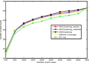
we compared MOClustering means, MOClustering medoids,
DM-76
Clustering, and RT-ms (RT with method sequence — a random
77
sequence generation approach for OOS test cases with method
Table 1: SUBJECT PROGRAMS
ID name
Lines of code
Num. of public classes
Num. of public methods
Num. of faults
Description
1 CCoinBox [32] 120 1 7 4 C++library that simulates a vending machine 2 WindShieldWiper [32] 233 1 13 4 C++library that simulates a windshield wiper 3 SATM [32] 197 1 9 4 C++library that simulates an Automatic Teller Machine 4 RabbitsAndFoxes [33] 770 6 33 9 C# program that simulates a predator-prey model 5 WaveletLibrary [34] 2406 12 84 15 C# library for wavelet algorithms
6 IceChat [34] 571000 101 271 24 C# program that implements an IRC (Internet Relay Chat) Client
7 CSPspEmu [35] 406808 443 1433 26 C# program for a PSP (PlayStation Portable) emulator
Table 2: MUTATION OPERATORS AND THE NUMBER OF FAULTS SEEDED
ID Num.of Mutation operators (number)
faults
1 4 AOR(1), LOR(2), ROR(1) 2 4 AOR(1), LOR(1), ROR(1), ACR(1) 3 4 AOR(1), LOR(1), ROR(1), SCR(1)
4 9 AOR(1), LOR(1), SVR(1), NMI(1), AOC(1), AMeC(1), AMoC(1), HVD(1), PRM(1)
LOR(1), SVR(1),CSR(2), SCR(1), ACR(2), 5 15 NMI(1), AOC(1), AMeC(1), AMoC(2), HVD(2),
PRM(1)
AOR(2), LOR(1), ROR(1), SVR(2),CSR(2), 6 24 SCR(1), ACR(2), NMI(2), AOC(3), AMeC(2),
AMoC(2), HVD(2), PRM(2) AOR(2), LOR(1), ROR(1),SVR(2),CSR(1), 7 26 SCR(1), ACR(2), NMI(2), AOC(3), AMeC(3),
AMoC(3), HVD(3), PRM(2)
invocation sequence),and Method Coverage (a method
cover-1
age TCP technique).
2
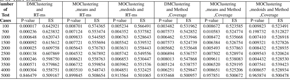
In order to properly assess the statistical significance of the
3
differences between our methods and other methods, we
con-4
ducted the effective statistical analysis based on the p-values
5
and effect size (set at a 5% level of significance)using the
un-6
paired two-tailed Wilcoxon-Mann-Whitney test and the
non-7
parametric Vargha and Delaney effect size measure [38–40].
8
The p-value is used to show the statistical significance of
d-9
ifference. If the p-value (probability value) is less than 0.05,
10
which means that there is significant difference between the
t-11
wo compared methods, otherwise not [38]. Additionally, we
12
used the non-parametric effect size (ES) measure to show the
13
probability that one method is better than another [39]. That is,
14
when we get the ES for any two methods A and B, a higher ES
15
value indicates higher probability showing A is better than B.
16
In this study, we used R language [41] to obtain the p-value and
17
ES value for the pair-wise TCP techniques.
18
5.3. Experimental parameters
19
For both theK-means and theK-medoids clustering
algo-20
rithms,Kis the main input parameter. If the value ofK is not
21
suitable, low quality clusters may be generated: if test cases are
22
clustered into too many clusters, then some similar test cases
23
may be put into different clusters; if they are clustered into too
24
few, then dissimilar test cases may be put into the same
clus-25
ter. Both of these situations may lead to poor failure detection
26
performance.
27
In this study, in order to find its most suitable value,Kwas
28
set to 2%, 5%, 10%, 15%, 20%, 25%, and 30% of the total
29
number of test cases (5000 test cases). Based on the overall
30
experimental results, appropriate values ofK for each subject
31
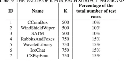
program were determined, as shown in Table 3.
[image:9.595.327.537.328.432.2]32
Table 3: THE VALUE OF K FOR EACH SUBJECT PROGRAMS Percentage of the
ID Name K total number of test
cases
1 CCoinBox 500 10%
2 WindShieldWiper 500 10%
3 SATM 500 10%
4 RabbitsAndFoxes 750 15% 5 WaveletLibrary 750 15%
6 IceChat 750 15%
7 CSPspEmu 750 15%
In addition, in all experiments (Fm,EandAPFD),testcase
-33
poolin Algorithms 1 to 3 simulated the input domain, and
T-34
Numin Algorithms 1 to 3 was the total number of test cases
35
(5000). The value ofn in Algorithm 4 was set to 100, 500,
36
1000, 1500, 2000, 2500, 3000, 3500, 4000 and 5000.
37
5.4. Experiments
38
To evaluate the effectiveness of our approaches, we
attempt-39
ed to answer the following three research questions:
40
RQ1: Do cluster TCP techniques perform better than
prior-41
itization with random sequences or method coverage, in terms
42
ofFm?
43
RQ2: Do cluster TCP techniques perform better than
prior-44
itization with random sequences or method coverage, in terms
45
ofE?
46
RQ3: Do cluster TCP techniques perform better than
prior-47
itization with random sequences or method coverage, in terms
48
of APFD?
49
5.4.1. Results and discussion
50
1)Do MOClustering means, MOClustering medoids and
DM-51
Clustering perform better than prioritization with random
se-52
quences and Method Coverage, in terms of Fm?
53
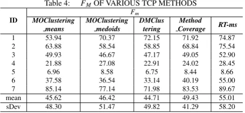
Table 4 summarizes the Fm results for the five different
54
methods. All results in the table were averaged over 100 runs of
55
tests for each subject program, each time with a different seed.
Table 4: FMOF VARIOUS TCP METHODS
ID
Fm
MOClustering means
MOClustering medoids
DMClus tering
Method
Coverage RT-ms
1 53.94 70.37 72.15 71.92 74.87
2 63.88 58.54 58.85 68.84 75.54
3 49.93 46.67 47.17 49.05 52.90
4 21.88 27.08 22.91 24.02 28.45
5 6.96 8.58 6.75 8.44 8.66
6 37.58 36.54 33.14 40.19 55.00
7 85.14 77.14 71.98 83.53 89.67
mean 45.62 46.42 44.71 49.43 55.01
sDev 48.30 51.47 49.82 41.29 58.20
Table 4 shows that, for the CCoinBox program,
MOCluster-1
ing means used the least number of test cases to detect the first
2
failure, followed by MOClustering medoids, Method Coverage,
3
DMClustering and RT-ms. For programs WindShieldWiper,
4
MOClustering medoids found the first fault with the least
num-5
ber of test cases, followed by DMClustering, MOClustering
me-6
ans, Method Coverage and RT-ms. For programs SATM,
MO-7
Clustering medoids found the first fault with the least number
8
of test cases, followed by DMClustering, Method Coverage,
9
MOClustering means and RT-ms. For the RabbitsAndFoxes
10
program, the number of test cases used by MOClustering means
11
and DMClustering to detect the first failure was similar, and less
12
than that for Method Coverage, MOClustering medoids and
RT-13
ms. For the WaveletLibrary, IceChat, and CSPspEmu
program-14
s, DMClustering used the least number of test cases to find
15
the first failure, and RT-ms used the most. For the
program-16
s IceChat and CSPspEmu, MOClustering medoids performed
17
better than MOClustering means and RT-ms, but for the
pro-18
gram WaveletLibrary, MOClustering means performed better
19
than Method Coverage, MOClustering medoids and RT-ms.
Th-20
erefore, in terms of the Fm, on average, DMClustering
per-21
formed best, especially for the large-scale programs, followed
22
by MOClustering means, MOClustering medoids, Method
Cov-23
erage and RT-ms. Compared with RT-ms, DMClustering
achie-24
ved an average of 18.72% improvement; MOClustering means
25
achieved an average of 17.07%; and MOClustering medoids
26
achieved an average of 15.62% improvement. Compared with
27
Method Coverage, DMClustering achieved an average of 9.55%
28
improvement; MOClustering means achieved an average of 7.71%;
29
and MOClustering medoids achieved an average of 6.09%
im-30
provement. Hence, the proposed cluster TCP techniques always
31
performed better than prioritization with random sequences and
32
method coverage prioritization, in terms ofFm.
33
In order to further analyze theFmof each testing method for
34
each subject program, Tables 4 and 5 also summarize the main
35
statistical measures includingsDev(standard deviation) for the
36
7 subject programs. The standard deviation for RT-ms is the
37
biggest (58.20), which indicates that its data points are spread
38
out over a wider range than other TCP techniques.
[image:10.595.42.288.91.204.2]39
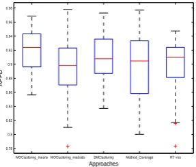
Figure 4 to 10 are box-plots diagrams showing theFm
re-40
sults for the seven subject programs, with the data in each
box-41
plot being theFmresults over 100 runs for each subject program
42
with different seeds.
43
MOClustering_means MOClustering_medoids DMClustering Method_Coverage RT−ms 0
50 100 150 200 250 300 350
Approaches
Fm
Figure 4:Fmexperimental results for CcoinBox
MOClustering_means MOClustering_medoids DMClustering Method_Coverage RT−ms 0
50 100 150 200 250 300 350 400
Approaches
[image:10.595.360.503.265.389.2]Fm
Figure 5:Fmexperimental results for WindShieldWiper
MOClustering_means MOClustering_medoids DMClustering Method_Coverage RT−ms 0
50 100 150 200 250
Approaches
[image:10.595.360.503.440.565.2]Fm
Figure 6:Fmexperimental results for SATM
MOClustering_means MOClustering_medoids DMClustering Method_Coverage RT−ms 0
20 40 60 80 100 120 140 160 180
Approaches
Fm
[image:10.595.358.503.617.739.2]Table 5: STATISTICAL RESULT OFFMFOR 7 SUBJECT PROGRAMS
ID MOClustering MOClustering DMClustering Method RT-ms
means medoids Coverage
1 mean 53.94 70.37 72.15 71.92 74.87
sDev 48.93 64.43 64.39 53.93 70.01
2 mean 63.88 58.54 58.85 68.84 75.54
sDev 61.27 66.24 57.75 48.59 71.40
3 mean 49.93 46.67 47.17 49.05 52.90
sDev 43.13 38.56 40.43 36.79 51.90
4 mean 21.88 27.08 22.91 24.02 28.45
sDev 17.37 24.50 20.80 16.42 29.32
5 mean 6.96 8.58 6.75 8.44 8.66
sDev 6.22 6.88 5.39 5.50 7.67
6 mean 37.58 36.54 33.14 40.19 55.00
sDev 34.09 35.88 34.57 34.13 39.36
7 mean 85.14 77.14 71.98 83.53 89.67
[image:11.595.42.556.283.363.2]sDev 53.06 56.03 54.40 60.42 61.91
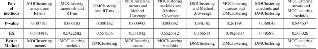
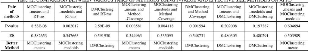
Table 6: COMPARISON BETWEEN VARIOUS PAIRS OF METHODS USING P-VALUE AND EFFECTIVE SIZE METHODS ONFM
Pair MOClustering MOClusterig MOClustering MOClustering DMClustering MOClustering MOClustering MOClustering of means and medoids and DMClusterig means and medoids and and Method means and medoids and means and
methods RT-ms RT-ms and RT-ms Method Method Coverage DMClustering DMClustering MOClustering
Coverage Coverage medoids
P-value 0.007193 0.006183 0.000192 0.000943 0.000692 1.64E-05 0.261891 0.360047 0.844637
ES 0.5434847 0.5422582 0.557556 0.551042 0.5523612 0.566514 0.4826837 0.485873 0.503026
Better MOClustering MOClustering
DMClustering MOClustering MOClustering DMClustering DMClustering DMClustering MOClustering
Method means medoids means medoids means
MOClustering_means MOClustering_medoids DMClustering Method_Coverage RT−ms 0
5 10 15 20 25 30 35 40
Approaches
[image:11.595.358.506.390.515.2]Fm
Figure 8:Fmexperimental results for WaveletLibrary
MOClustering_means MOClustering_medoids DMClustering Method_Coverage RT−ms 0
50 100 150 200
Approaches
[image:11.595.91.234.570.691.2]Fm
Figure 9:Fmexperimental results for IceChat
MOClustering_means MOClustering_medoids DMClustering Method_Coverage RT−ms 0
50 100 150 200 250 300
Approaches
Fm
Figure 10:Fmexperimental results for CSPspEmu
As can be observed from Figure 4, both the outlying and the
1
maximum observed values of MOClustering means are far
s-2
maller than corresponding values of RT-ms. Figure 5 shows that
3
the performances of the five methods are similar, but the
medi-4
ans of MOClustering means, MOClustering medoids and
DM-5
Clustering are much smaller than the medians of Method Coverage
6
and RT-ms. This implies that in most cases, Method Coverage
7
and RT-ms required more test cases to find the first fault. As
8
shown by Figure 6, three cluster TCP techniques outperform
9
other methods with smaller medians. As observed from
Fig-10
ure 7, the performances of MOClustering medoids,
MOClus-11
tering means, DMClustering, and Method Coverage are
simi-12
lar, while they outperform RT-ms with larger outlying point
val-13
ues and maximum values. As seen from Figures 8 and 10,
DM-14
Clustering has the shorter IQR (interquartile range) and smaller
15
medians than Method Coverage and RT-ms, which means that
16
its performance is more stable than that of these two methods