doi:10.1017/S0022112006002412 Printed in the United Kingdom
Effect of Mach number on the structure
of turbulent spots
By L. K R I S H N A NA N D N. D. S A N D H A M Aeronautics and Astronautics, School of Engineering Sciences,
University of Southampton, SO17 1BJ, UK
(Received1 June 2006 and in revised form 10 August 2006)
Direct numerical simulations have been performed to study the dynamics of isolated turbulent spots in compressible isothermal-wall boundary layers. Results of a bypass transition scenario at Mach 2, 4 and 6 are presented. At all Mach numbers the evolved spots have a leading-edge overhang, followed by a turbulent core and a calmed region at the rear interface. The spots have an upstream-pointing arrowhead shape when visualized by near-wall slices, but a downstream-pointing arrowhead in slices away from the wall. The lateral spreading of the spot decreases substantially with the Mach number, consistent with a growth mechanism based on the instability of lateral shear layers. Evidence for a supersonic (Mack) mode substructure is found in the Mach 6 case, where coherent spanwise structures are observed under the spot overhang region.
1. Introduction
The breakdown of a laminar boundary layer into turbulence often occurs via the formation of localized turbulent patches, referred to as turbulent spots. These spots grow as they are convected downstream and eventually merge into a fully turbulent boundary layer. The length of the transition region depends on spot characteristics such as the convection speed of the leading and trailing edges of the spot, the lateral growth rate and any interactions between spots (Krishnan & Sandham 2006). A mature turbulent spot is depicted in figure 1(a), showing the arrowhead-shaped spot core with a leading-edge overhang. Lateral growth from the spot wingtips is measured by the spreading half-angle β = tan−1(b
(a) (b)
Streaks
6
3
3 2 1
2 4
5 1
[image:2.493.67.445.55.165.2]Flow β
Figure 1.Turbulent spot nomenclature: (1) front overhang, (2) turbulent core, (3) lateral
wingtip, (4) calmed region, (5) lateral spreading half-angle (β), (6) spanwise overhang, seen in endview. (a) Schematic outline. (b) Spot flow visualization showing the sublayer streaks. (Cantwellet al.1978).
nonlinear interactions and breakdown of these hairpin structures, resulting in the formation of a fully turbulent flow field. The growth mechanism of a spot in a boundary layer is complex, since the spot interacts with the irrotational free-stream flow above it and the rotational laminar boundary layer flow surrounding it. The physical mechanisms involved in the lateral and wall-normal growth of a spot are different. The wall-normal growth of the spot is similar to the classical entrainment mechanism, while the difference between convective speeds of the front and the tail of a spot results in the spot growth in the streamwise direction. Spots are believed to grow in the lateral direction by destabilizing the surrounding laminar flow, rather than by turbulent diffusion (Gad-el-Hak, Blackwelder & Riley 1981).
Most of the earlier studies on turbulent spots were performed for incompressible flows (see for example Narasimha 1985; Wygnanski, Zilberman & Haritonidis 1982), with relatively few studies of the effect of compressibility. Variation of the wall and lateral spreading angles of the disturbance region with local Mach number was reported by Fischer (1972), who also summarized the results of earlier experiments. The spreading angle relative to the wall remained invariant with Mach number while the lateral spreading angle decreased sharply fromβ= 10◦−11◦to 3◦with increasing Mach number(M) up to M = 6. Clark, Jones & LaGraff (1994) found a decrease in the lateral spreading of the spot with a favourable pressure gradient and also with increasing M (β = 9.9◦ for M = 0.24 and β = 6◦ for M = 1.32). Most recently, in boundary layer transition experiments using thin-film heat-transfer gauges atM = 6, Mee (2002) also demonstrated that turbulent spots grow with a more slender angle (β = 3.0◦) than at low M. Most of the available experimental results are based on ensemble-averaged flow field measurements. The present computational study has been carried out to provide a more complete picture of the effects of compressibility on spot characteristics.
2. Simulation details
A high-order scheme is used to solve the time-dependent compressible Navier– Stokes equations for flow variables (ρ, ρui, ρE), whereρis the density,ui are velocity
Case Mach Re∗δ
in Tw/T∞ (Lx, Ly, Lz)/δ
∗
in Nx, Ny, Nz
M2 2 950 1.67 400×60×60 801×101×121
M4 4 2000 3.69 450×60×60 801×101×121
M6 6 3000 7.00 600×30×40 601×101×121
Table 1. Details of spot simulations.
third-order Runge–Kutta method. Details of the shock-capturing and entropy-splitting algorithms can be found in Yee, Sandham & Djomeri (1999) and Sandham, Li & Yee (2002). An additional filter (Ducroset al.1999; Krishnan & Sandham 2006) is applied to turn off the shock-capturing scheme within most of the boundary layer. All lengths are normalized with the displacement thickness (δ∗in) of the laminar inflow profile, which is obtained by a separate self-similar compressible boundary layer solution. Velocity, temperature, density and viscosity are normalized with free-stream values at the inflow. Details of the various cases considered are given in table 1. The flow is assumed to be periodic in the spanwise direction and a no-slip fixed-temperature wall condition is applied at the plate surface. Characteristic boundary conditions are used at the inflow, outflow and upper surface. The laminar base flow is perturbed by a localized injection of low-momentum fluid through a spanwise symmetric rectangular slot of dimensions 4 × 4 (x, z) centred at x= 22, z=Lz/2. The blowing trip is
applied for a short duration of 8 non-dimensional time units (δ∗in/u∞) by specifying the vertical velocity at the plate surface as vinj = Au∞; the amplitude A of the disturbance is chosen such that a spot can be efficiently triggered and studied within the present computational domain. The blowing trip used here has previously been used in experiments such as Perry, Lim & Teh (1981) and Gad-el-Hak et al. (1981). Fully developed spots are believed to be independent of the method of initiation (Singer 1996). A perturbation amplitude of A = 0.2 was used for the Mach number M = 2 and 6 cases. For the M = 4 case the length of the injection slot was 6 and the value of A was set to 0.35. The maximum local mean friction velocity (uτ =
√
µw(du/dy)w/ρw, with subscript w denoting the wall, and mean properties refer to
the spanwise-averaged flow properties in the spot core) is found to be around 0.055 for the spot cases considered. The estimated grid resolution in viscous wall units is x+ = 7.5–12.5, z+ = 7.5–12.5 based on the maximum mean friction velocity at the wall, suggesting that the spot turbulence is properly resolved in the simulation. The present grid resolution is also comparable to other DNS studies in the literature (for example Maeder, Adams & Kleiser 2001).
3. Results
3.1. Effect of Mach number
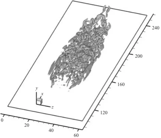
The large-amplitude disturbances trigger an incipient spot downstream of the injection slot as shown by a surface of Π = (∂ui/∂xj)(∂uj/∂xi) on figure 2. The organization
0
20
40
60
120 160
200 240
y x
[image:4.493.123.386.63.289.2]z
Figure 2. Iso-surface of the second invariant of the velocity gradient tensor att= 249; M= 2 (Π=−0.0008).
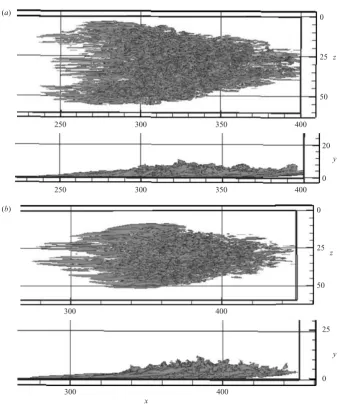
the evolved turbulent spot are shown in figures 3(a) and 3(b) at M = 2 and M = 4 respectively. Near-wall streaky structures are clearly visible in the present DNS, as in flow visualization studies on incompressible spots (Cantwellet al. 1978; Gad-el-Hak et al. 1981).
In high-Mach-number boundary layers there can be additional inviscid modes (Mack 1977). The mechanism for instability involves reflection of acoustic waves between the solid surface and the sonic line. At low Mach numbers the subsonic mode (first mode) instabilities play a major role in destabilizing the flow. However, aboveM= 3.8 the larger amplification rate of the inviscid instabilities (Mack modes) means that they can dominate the first mode instabilities. In this context we note that in the M = 6 spot, shown on figure 4, breakdown to turbulence is markedly different to that at M = 2 and 4. In particular we note the appearance of coherent spanwise structures close to wall, visible for example in the side view of figure 4 under the spot overhang. The location and form suggest an underlying mechanism similar to the Mack modes. Fiala et al. (2006), in their hypersonic transitional boundary layer experiments on a blunt cylinder model at M = 8.9, observed cell-like patterns in the surface heat transfer footprints associated with a spot. Figure 4 suggests that the cell-like patterns may be associated with the development of Mack mode substructures.
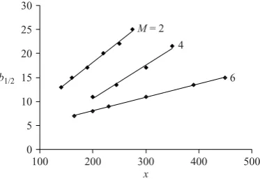
The lateral growth of a spot is highly dependent on the flow Mach number. Figure 5 shows the evolution of the spot half-width (b1/2), which is determined using plan views of the three-dimensional wall-normal vorticity contours (ωy =±0.06). The estimated
400 350
300 250
0
25
50
400 350
300 250
20
0 z
y
400 300
0
25
50
400 300
25
0 z
y (a)
(b)
[image:5.493.70.409.53.463.2]x
Figure 3. Iso-surface of wall-normal vorticity,ωy=±0.06. (a)M= 2,t = 451, (b)M= 4, t= 475.
Case ufront utail uwt β(deg.)
M2 0.87 0.53 0.57 5.0±0.2
M4 0.87 0.59 0.76 4.0±0.2
M6 0.89 0.68 0.76 1.7±0.2
Table 2.Results of spot simulations.
0
10
20
30
40 0 550 500
450 400
550 500
450 400
z
30
20
10
0 y
[image:6.493.76.435.51.255.2]x
Figure 4. Iso-surface of the second invariant showing the Mack mode structures;M= 6,
t= 562,Π=−0.0008.
30
25
20
15
10
5
0
100 200 300 400 500
x b1/2
M = 2 4
6
Figure 5. Variation of spot half-width (b1/2) with axial locationx.
3.2. Spot structure
[image:6.493.161.348.300.428.2]50 (a)
(b) 25
0 0
25
50 200
250
300
350
400
y
y
x x
z
Calmed region
20
15
10
5
0 10 20 30 40 50 60
Lateral overhang region y
[image:7.493.90.392.59.414.2]z
Figure 6. Iso-surface of the streamwise velocity perturbations att= 390 (M= 4); u=±0.02); (a) three-dimensional view, (b) side view.
varying the wall distance within the same spot, irrespective of the origin of the spot. The smaller spot spreading angles obtained by the surface heat transfer experiments of Zhong et al. (2000) are similarly explained by the vertical variations in structure; the lateral overhang means that surface measurements do not represent the width of the spot as would be seen in a plan view.
In the present simulations wall heat transfer is highly dependent on location within the spot. A local wall heat transfer coefficient may be defined by
ch=
qw∗
ρ∗u∗∞cp∗(T0∗−Tw∗), (3.1) where qw =−κ(∂T /∂y)w is the wall heat transfer rate, κ is the thermal conductivity,
T0 is the stagnation temperature and an asterisk denotes a dimensional quantity. The M = 2 simulation has been used to give some typical values. In the laminar region and under the front overhang of the spot ch = 0. In the calmed region behind the
60
40
20
0
200 250 300 350
(a)
(b)
(c) 60
40
20
0
200 250 300 350
60
40
20
0
200 250 300 350
z
z
z
[image:8.493.133.374.49.333.2]x
Figure 7.Two-dimensional slices of the streamwise velocity perturbations at various wall-normal positions,t= 390 (M= 4);u=±0.02); (a)y= 0.16, (b)y= 1.63, (c)y= 4.65.
(see figure 3a). In the rear portion of the turbulent core the heat transfer changes sign, reaching a minimum of ch ≈ −0.003 (wall heating) at x ≈ 300. The level of
ch then ramps upwards through the spot, with peak heat transfer occurring at the
front of the turbulent core, with ch ≈ 0.004 at x ≈ 335. In connection with these
observations we note that within the turbulent core there are competing effects of turbulent dissipation, leading to locally increased temperature close to the wall, and turbulent diffusion, which brings cool fluid towards the wall.
3.3. Intermittency function
In modelling flow transition, the extent of the transition region is described using an intermittency distribution. Based on the hypothesis of concentrated breakdown, i.e. that spots form at a preferred streamwise location randomly in time and cross-stream position, Dhawan & Narasimha (1958) used the universal intermittency distribution function to characterize the transition zone:
γ(x) = 1−exp [−(x−xt)2nσ/u∞](x>xt)
= 0 (x6xt). (3.2)
Heren is the breakdown rate (spots occurring per unit time at the location xt) and
σ is the spot propagation parameter
σ = u∞t x3
x
xo
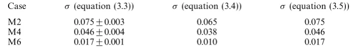
Case σ (equation (3.3)) σ (equation (3.4)) σ (equation (3.5))
M2 0.075±0.003 0.065 0.075
M4 0.046±0.004 0.038 0.046
[image:9.493.64.414.69.120.2]M6 0.017±0.001 0.010 0.017
Table 3.Comparison of different methods of computing the non-dimensional spot
propagation parameter σ.
where b1/2 is the half-width of the spot and xo is the virtual origin of the spot. The
accuracy of any transition model using the above intermittency distribution function mainly depends on the value ofnσ. In most of the previous transition studies attempts were made to fit the data to the universal intermittency function, which has resulted in correlations for nσ in a variety of flows. It is not possible to estimate nfrom the present isolated spot study, but the value of σ can be computed directly. Narasimha (1985) found that 2σ (i.e. using the full spot width in (3.3)) takes a value around 0.25 near the wall and 0.29 away from the wall (the variation is due to the spanwise overhang). He also estimated 2σ ≈ 0.05 at M= 6 using the data of James (1958). Vinod & Rama (2004) in their recent transition studies definedσ as a function of the lateral spreading half-angle β and the convective speeds of the front (ufront) and the tail (utail) of the spot:
σ =
1 utail
− 1 ufront
u∞tanβ. (3.4)
In this study it is more appropriate to define σ based on the spreading half-angle β and the convective speed of the spot wingtip (lateral extremity of the spot):
σ = 1 2
u∞ uwt
tanβ, (3.5)
where uwt is the convective speed of the wingtip. A comparison of the σ values estimated using equations (3.3), (3.4) and (3.5) is shown in table 3. The present definition (3.5) of the non-dimensional spot propagation parameter σ shows good agreement with the integral definition of Narasimha (1985). This reduction in σ is also consistent with the spreading half-angles given in table 2, indicating that compressibility enters primarily via theσ parameter.
4. Summary
with previous experimental results and provide additional data on turbulent spot celerities in compressible flows. The effect of compressibility is found mainly to suppress the spot propagation parameterσ.
The authors would like to acknowledge the financial support of the European Space Agency (ESA-ESTEC) for this work, under contract 17531/03/NL/SFe, technical officer Dr J. Steelant.
R E F E R E N C E S
Cantwell, B., Coles, D. & Dimotakis, P.1978 Structure and entrainment in the plane of symmetry of a turbulent spot.J. Fluid. Mech.87, 641–672.
Clark, J. P., Jones, T. V. & LaGraff, J. E.1994 On the propagation of naturally-occurring turbulent spots.J. Engng Maths 28, 1–19.
Dhawan, S. & Narasimha, R.1958 Some properties of boundary layer flow during transition from laminar to turbulent motion.J. Fluid. Mech.3, 418–436.
Ducros, F., Ferrand, V., Nicoud, F., Weber, C., Darracq, D., Gacherieu, C. & Poinsot, T.1999 large-eddy simulation of the shock/turbulence interaction.J. Comput. Phys.152, 517–549. Fiala, A., Hillier, R., Mallinson, S. G. & Wijesinghe, H. S.2006 Heat transfer measurement of
turbulent spots in a hypersonic blunt-body boundary layer.J. Fluid Mech.555, 81–111. Fischer, M. C.1972 Spreading of a turbulent disturbance.AIAA J.10(7), 957–959.
Gad-el-Hak, M., Blackwelder, R. F. & Riley, R. J.1981 On the growth of turbulent regions in laminar boundary layers.J. Fluid Mech.110, 73–95.
Haidari, A. H. & Smith, C. R.1994 The generation and regeneration of single hairpin vortices.
J. Fluid Mech.277, 135–162.
James, C. J.1958 Observations of turbulent burst geometry and growth in supersonic flow.NACA
Tech. Note4325.
Krishnan, L.2005 Dynamics of turbulent spots in a compressible flow. PhD Thesis, University of Southampton, UK.
Krishnan, L. & Sandham, N. D.2006 On the merging of turbulent spots in a supersonic boundary-layer flow.Intl J. Heat Fluid Flow27, 542–550.
Mack, L. M. 1977Transition prediction and linear stability theory,Agard CP224. NATO, Paris. Maeder, T., Adams, N. A. & Kleiser, L.2001 Direct simulation of turbulent supersonic boundary
layers by an extended temporal approach.J. Fluid Mech.429, 187–216.
Mee, D. J.2002 Boundary-Layer transition measurements in hypervelocity flows in a shock tunnel.
AIAA J.40(8), 1542–1548.
Narasimha, R.1985 The laminar-turbulent transition zone in the boundary layer.Prog. Aero. Sci. 22, 81–111.
Papamoschou, D. & Roshko, A. 1988 The compressible turbulent shear layer: an experimental study.J. Fluid Mech.197, 453–477.
Perry, A. E., Lim, T. T. & Teh, E. W.1981 A visual study of turbulent spots.J. Fluid Mech. 72, 731–751.
Sandham, N. D., Li, Q. & Yee, H. C.2002 Entropy splitting for higher-order numerical simulation of compressible turbulence.J. Comput. Phys.178, 307–322.
Singer, B. A.1996 Characteristics of a young turbulent spot.Phys. Fluids 8(2), 509–521.
Vinod, N. & Rama, G.2004 Pattern of breakdown of laminar flow into turbulent spots.Phys. Rev.
Lett.93(11), 114501-1-4.
Wu, X., Jacobs, R. G., Hunt, J. C. R. & Durbin, P. A.1999 Simulation of boundary layer transition induced by periodically passing wakes.J. Fluid Mech.398, 109–153.
Wygnanski, I., Zilberman, M. & Haritonidis, J. H.1982 On the spreading of a turbulent spot in the absence of a pressure gradient.J. Fluid Mech.123, 69–90.
Yee, H. C., Sandham, N. D. & Djomeri, M. J. 1999 Low-dissipative high-order shock-capturing methods using characteristic-based filters.J. Comput. Phys.150, 199–238.