Transient dynamics of heterogeneous micro grids using second order consensus

This is a repository copy of

Transient dynamics of heterogeneous micro grids using

second order consensus

.

White Rose Research Online URL for this paper:

http://eprints.whiterose.ac.uk/144275/

Version: Accepted Version

Proceedings Paper:

Genis Mendoza, F., Bauso, D. and Namerikawa, T. (2017) Transient dynamics of

heterogeneous micro grids using second order consensus. In: 2017 International

Conference on Wireless Networks and Mobile Communications (WINCOM). 2017

International Conference on Wireless Networks and Mobile Communications (WINCOM),

01-04 Nov 2017, Rabat, Morocco. IEEE . ISBN 978-1-5386-2123-3

https://doi.org/10.1109/WINCOM.2017.8238210

[email protected] https://eprints.whiterose.ac.uk/ Reuse

Items deposited in White Rose Research Online are protected by copyright, with all rights reserved unless indicated otherwise. They may be downloaded and/or printed for private study, or other acts as permitted by national copyright laws. The publisher or other rights holders may allow further reproduction and re-use of the full text version. This is indicated by the licence information on the White Rose Research Online record for the item.

Takedown

If you consider content in White Rose Research Online to be in breach of UK law, please notify us by

Transient Dynamics of Heterogeneous Micro Grids

Using Second Order Consensus

1

Fernando Genis Mendoza

and Systems Engineering The University of Sheffield Mappin Street, S1 3JD Sheffield

United Kingdom

Email: [email protected]

2

Dario Bauso

and Systems Engineering The University of Sheffield Mappin Street, S1 3JD Sheffield

United Kingdom Email:[email protected]

3

Toru Namerikawa

Department of System Design Engineering Keio University

Yokohama, 223-8522, Japan Email: [email protected]

Abstract_{—This paper deals with a network of interconnected}

micro grids. The transient dynamics is modelled as an averaging process involving dynamic agents in a network. An analysis of the convergence of the consensus dynamics is provided using a network model based approach and by exploiting the properties of the corresponding graph-Laplacian matrix. Furthermore an investigation of the transient dynamics is carried out for different damping and inertial parameters and under different time-varying topologies. Finally a simulation is performed based on a model calibrated on an existing network in the UK under parameter uncertainties.

I. INTRODUCTION

This paper provides an analysis of the transient dynamics of a network of micro grids. A micro grid is modelled using the swing dynamics and involving both damping and inertial parameters. The interaction between micro grids is modelled using the coupled oscillator paradigm and the resulting dynam-ics is captured by a Laplacian matrix. The transient analysis is extended to time-varying topologies to gain insight on the role of connectivity.

A. Main Contributions

As first result, similarities between the transient stability and consensus dynamics are emphasized under the assumption of homogeneity between micro grids. This result also shows how different damping coefficients affect the frequency and the power flow consensus values. Stability analysis for the heterogeneous case is performed by estimating the system’s eigenvalues and through the analysis based on the Gershgorin theorem and the Nyquist stability theorem. Simulations are carried out using different topologies to gain insight on how the connectivity of the network affects the time constant of the transient response of the system. The analysis is then extended to the case where the parameters of each micro grid are uncer-tain and subject to change over time, thus providing a better understanding of the resilience of the network. The present work involves also the adaptation of a network topology to real instances and the calibration of the nodes’ parameters using data of the power capabilities of each micro grid.

B. Reviewed Literature

The role of the Laplacian in the swing dynamics and the analogy with the Kuramoto coupled oscillator model is studied in [1]. The model based on the swing dynamics and the link with the Laplacian for small phase angles is discussed in [2]. Modelling design of a network of interconnected oscillators and the influence of disturbances is studied in [3]. Transient analysis on coupled oscillators and the relation between damp-ing and inertial coefficients is investigated in [4]. The role of the damping parameters in a network of electrical generators is discussed in [5]. The examples of existing UK electrical network topologies and parameters in this paper are obtained from [6]. Parameter approximation for electrical networks and their use in the swing equations is studied in [7] and references therein.

This paper is organized as follows. In section II we state the problem and introduce the model. In Section III we present the main results. In Section IV we provide simulations. Finally in Section V we provide conclusions and discuss future directions.

II. PROBLEMSTATEMENT ANDMODEL

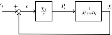
The model of a single micro grid i in a network involves the dynamics of the power flow in the micro grid, denoted by Pi which is given by,

˙

Pi=Ti j(fj−fi), (1)

where fiis the frequency of gridi, fj is the frequency of grid j and Ti j is the synchronizing coefficient which is obtained as the inverse of the line impedance between gridsi and j. If micro gridi is connected to multiple other micro grids, then the variable fj can also represent the average frequency over the neighbour micro grids of micro grid i.

fj +

−

e Ti j

s

1 Mis+Di

fi Pi

Fig. 1. System block representation of micro gridi.

also involves the dynamics for the frequency fi which is in accordance with the following swing equation:

˙ fi=−

Di Mi

fi+ 1 Mi

Pi, (2)

whereDidenotes the damping coefficient of micro gridiand Miis its inertial coefficient. Figure 1 shows the system block representation of the dynamic system (1)-(2).

The state space representation of the system can be obtained by introducing the state variablesPi=x(

i) 1 , fi=x(

i)

2 and taking fj =x(₂j) as an external input. Model (1)-(2) can then be rewritten in compact form as:

"

˙ x(₁i)

˙ x(₂i)

#

=

0 −Ti j 1 Mi −

Di

Mi "

x(₁i) x(₂i)

#

+

Ti j 0

x(₂j). (3)

A system of interconnected micro grids can be represented using a graphG. Each node represents a micro grid and each edge represents the power line that connects two micro grids; the connectivity of each node is the degree of the node and is denoted bydi. In the unweighted and undirected casedi is equal to the number of edges that are incident to node i.

Using the model in (3) and extending it to the case of a system of n micro grids we obtain the following state space representation             ˙ x(₁1)

.. . ˙ x(₁n)

˙ x(₂1)

.. . ˙ x(₂n)

            =           

0 ··· 0 −T11 ··· T1n . .. . .. 0 ··· 0 Tn1 ··· −Tnn 1

M1 ··· 0 − D1

M1 ··· 0

0 . .. 0 0 . .. 0 0 ··· 1

Mn 0 ··· −

Dn Mn                       

x(₁1) .. . x(₁n)

˙ x(₂1)

.. . x(₂n)

            (4) The block matrix that contains the synchronization param-eters Ti j can be linked to the graph-Laplacian matrix, which we define as

L:=



 

T11 ··· −T1n . ..

−Tn1 ··· Tnn





, (5)

where its diagonal entries correspond to the sum of the weights of the outgoing edges, while the off-diagonal entries are the weights of the adjacency matrixAof the network. Let us recall that the Laplacian of a graph is defined as

L=Dout−A, (6)

whereDout is a diagonal matrix whose elements are the out-degree of the nodes.

The Laplacian matrix is then used to represent the system dynamics in matrix form corresponding to (4) as follows

_˙ X1 ˙ X2 =

0 −L

Diag(_M1

i) −Diag(

Di

Mi)

X1 X2

, (7)

whereDiag(Di

Mi)denotes the diagonal matrix with main

diago-nal entries equal to the damping to inertia ratio andDiag(1 Mi)

is the diagonal matrix with main diagonal entries equal to the inverse of the inertial constant Mi of each micro gridi. The state variablesX1andX2are the vectors of power flowsPiand frequencies fi of each micro grid ifor i=1, . . . ,n.

For an unweighted, undirected network of heterogeneous grids with inertial coefficientsMiand damping coefficientsDi, to find the eigenvalues of system (7), the roots ofdet(λI₋A) must be obtained, where A is the matrix in (7). Rewriting A as a block matrix composed by four square matrices, and recalling that the determinant of a block matrix is obtained as:

det(

A B C D

) =det(D)det(A−BD−1C), ifDis invertible,

then we obtain

det(λI₋A) =det(

_{λI −L}

Diag(_M1

i) λI+Diag(

Di

Mi)

)

=det(λI+Diag(Di Mi

))det(λI+L(λI+Diag(Di Mi

)−1Diag( 1 Mi

)

=det(λ2I+λDiag(Di Mi

) +Diag(1 Mi

)L).

(8)

Denoting Ψ:=Diag(Di

Mi) and Φ:=Diag(

1

Mi) the system

matrixAand (8) can be rewritten as:

A=

0 −L

Φ ₋Ψ

, (9)

det(λI₋A) =det(λ2I+λΨ+ΦL). (10) From Nyquist stability theory, all eigenvalues λi must be located in the left half plane of the complex plane for the system to be stable. The following results illustrate how an estimation of the eigenvalues of systemAcan be obtained.

III. MAINRESULTS

A. Influence of Damping

Let us start by noting that A contains an eigenvalue in zero with multiplicity m which is obtained from the first m rows. Assuming Di>0 and Mi=M for all i and utilising the Gershgorin circle theorem, we can obtain a disc ∆_i which encloses the position of the eigenvalueλiin the complex plane. In this specific case, the disc∆_i is defined as

∆_i(−D_Mi, 1

M) ={ξ:ξ∈C| |ξ+ Di

M| ≤R}, (11) where

R=

∑

i6=j

|Qi j|= 1

M. (12)

Every disc ∆_i has a radius equal toR= 1

M and is centered in−Di

M on the real axis in the complex plane. Let us recall that the spectrum of Ais the set of eigenvalues{λ1,λ2, . . . ,λm}.

Theorem 1: For the spectrum of matrix A we have

spec(A)∈ [

i=1,...,m

∆i(− Di Mi

, 1

Mi

). (13)

For the sake of simplicity, let us assume that the nodes are ordered decreasingly in the damping to inertia ratio, namely

−_MDm

m

<−Dm−1

Mm₋1

. . . <−D2

M2

<−D1

M1

. (14)

In other words the ratio −D1

M1 contains the smallest damping

coefficient.

Corollary 1.1: The system (7) is stable if

1−D1 M1

<0. (15)

The above corollary establishes stability under the condition that all discs are in the left half complex plane. This is guaranteed once we obtain that the disc closest to the origin is in the left half plane. The value 1−D1

M1 is the distance of that

disc from the origin in the left half plane. Let us define

λ₁:=1−D1 M1

, (16)

then the following corollary holds.

Corollary 1.2: The value λ₁upper bounds the real part of the second smallest eigenvalue:

ℜ(λ1)≤λ1. (17)

Sinceλ_iis the second smallest eigenvalue, its rate of decay is dominant for the system’s response. In other words, the system’s response is exponentially bounded byλ₁namely the system converges to an equilibrium xeq as described by (18),

|x(t)−xeq| ≤ϒmeλ1t, (18)

whereϒ_m is an opportune 1×mvector.

B. Influence of Inertia

In this section two cases are analysed. For the first one it is assumed that Di

Mi =1, andMi=1 for alliso thatΦ=Ψ=

I_∈Rm_{. Then (10) can be rewritten as:}

det(λI₋A) =det((λ2_I+λ)I+L) =

∏

i

((λ2_I+λ)I+η

i),fori=1, . . . ,m. (19)

In the above equation ηi denotes the ith eigenvalue of −L. Taking the determinant in (19) equal to zero, the eigenvalues of A, which we denote by λi are then obtained as

λi,i+1=−

1±√1+4ηi

2 ,fori=1, . . . ,m. (20) From (20) and from the fact that by definition all ηi≤0, it can be deduced thatℜ(λi) is negative for all eigenvalues, hence the network system is stable.

For the second case, it is assumed that Di

Mi =1 for alli, so

that Ψ=I_∈Rm_{, (10) can now be rewritten as:}

det(λI₋A) =det((λ2_I+λ)I+ΦL) =

∏

i

((λ2_I+λ)I+µ˜

i),fori=1, . . . ,m, (21)

where ˜µi denotes theith eigenvalue of−ΦL. The eigenvalues of A, are then given by

λi,i+1=−

1±√1+4 ˜µi

2 ,fori=1, . . . ,m. (22) Since matrix Φ is diagonal, ΦL is obtained from the Laplacian matrixL by scaling each of its rowsli by _M1_i

ΦL =



  

l11 M1 ···

l1m

M1

. .. lm1 Mm ···

lmm

Mm 

  

=



 

1 M1l1

.. . 1 Mmlm



 . (23)

The scaling of the Laplacian shifts the Gershgorin discs of the eigenvalues closer to the origin in the complex plane.

C. Clusterization

Condition (14) yields the inequality

1−Di Mi

<1−Di+1

Mi+1

,for anyi_{∈ {}1, . . . ,m_}, (24)

where the left hand side describes the minimum distance of a point in ∆i from the origin, and the right hand side is the maximum distance of any point in ∆_i+1 from the origin. Let us now explore the case where two or more discs overlap (partially or completely). The union of the area of the overlapped discs can be referred to as acluster. For instance, a cluster containing the firstidiscs is disjoint from the cluster containing the lastn₋1 discs if

i

[

j=1

∆_j(−Dj,1)∩ n

[

j=i

The above condition means that the union of the first i discs{∆₁, . . . ,∆i}is disjoint from the union of lastn−idiscs

{∆_i+1, . . . ,∆n}. The number of clusters is obtained using the indicator function I_{, as follows}

∑

i

I₍

i

[

j=1 ∆_j∩

m

[

j=i

∆_j=/0). (26)

It is worth mentioning that when we have a sufficiently small Mi, (2) can be approximated as Difi=Pi from which we obtain

Dif˙i=Ti j(fj−fi). (27) System (7) reduces then to

diag(Di)f˙=−L f, (28) which implies

˙

f=−diag(1 Di

)L f. (29)

The above has the form of a consensus system characterized by a scaled Laplacian similar to the one in (23). Its Gershgorin discs can be obtained in a similar fashion as discussed in Section III-B.

IV. SIMULATIONS

In this section, real instances of power network topologies are simulated. The first one covers the case when the network is considered homogeneous, unweighted and undirected. The second example enables the analysis of the systems dynamics with a different network configuration and the influence of the connectivity on the response. Finally the third set of simulations were formulated to accommodate parameter uncer-tainties, in which case the network is heterogeneous, weighted and directed.

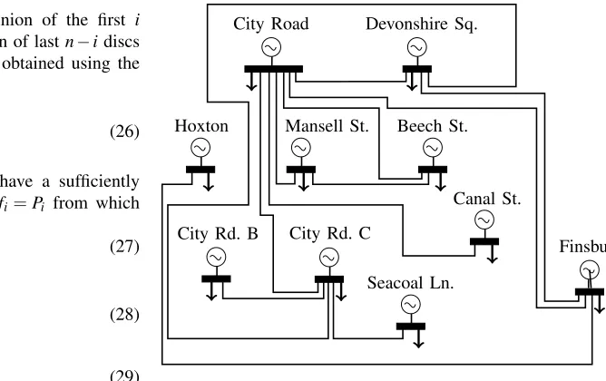
A. Graph Modelling from Existing Network

To support the theoretical analysis, simulations were done using real data of the London City Road electrical power network reported in [6]. Figure 2 illustrates the simplified one-line diagram that contains the geographical location and names of the generators and their respective load buses.

From the one-line diagram, a network topology graph was obtained as displayed in Fig. 3 the graph was modelled as unweighted and undirected as the influence between any two nodes is bidirectional. The graph is composed by 10 nodes and 13 edges.

The aim of the first set of simulations is to analyse the tran-sient dynamics and investigate convergence of the frequency and power of each micro grid to a desired reference. When this occurs, we say that the network achieves synchronization. In the present simulations, all micro grids are assimilated to homogeneous oscillators. The respective parameters were selected as follows: number of nodesn=10, inertial constant Ii=1, synchronizing coefficient Ti j=1, number of iterations N =6000, step size dt =0.01 seconds. Different damping constants Di=1,5,10 are used for different runs. Also the initial states of the frequency and power are obtained as

City Rd. C City Rd. B

Beech St. Mansell St.

Hoxton

Seacoal Ln. Devonshire Sq. City Road

Canal St.

Finsbury

Fig. 2. One-line diagram of part of the London City Road Network [6].

Hoxton Finsbury Canal St.

Seacoal Ln. Beech St. City Rd

Mansell St.

Devonshire Sq. City Rd. C

City Rd. B

Fig. 3. Graph topology analogous to the electrical network.

random values in the interval [0,1]. Frequency and power

variables are also reset every 20 seconds as a way to simulate periodic disturbances. The resulting plots have been scaled around 50 Hz and 30 MWh for the frequency and power flow respectively to approximate realistic values.

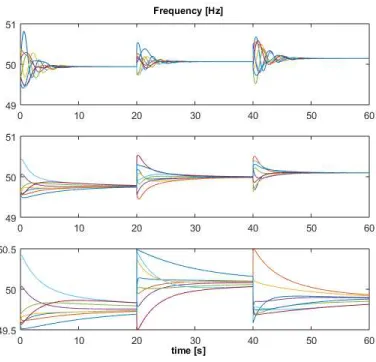
Figure 4 shows the frequency response of each micro grid. It can be seen that the response remains in the range between [49.5,50.5] Hz and thus it does not exceed in magnitude the

desired frequency by more than 1 Hz.

Figure 5 displays the power flow of each micro grid across time, in the same manner as the frequency, the values remain in the range of[29.5,30.5] MWh.

In both plots the different values of the damping constant are used from top to bottom. Observe that for larger values the oscillations are reduced but the settling time increases.

B. Changing the Topology

Fig. 4. State of the micro grid frequency over time.

Fig. 5. State of the power flow in each micro grid over time.

connections per node, in contrast to the 2.5 of the previous example.

Bankside B3 New Cross Canal St.

Charing Cross

Bankside C

Newington House Bankside F

Bankside D

Fig. 6. Derived graph for a different section of the Network

The network is considered unweighted and undirected. The rest of the parameters are left unchanged. The plot of the simulated frequency response can be seen in Figure 7.

Fig. 7. Frequency response in a different topology.

Comparing these results against the response from the first set of simulations in Figure 4, it can be seen that under the second topology the system converges about 2 seconds faster. This is more evident in the plots where Di=5. It is also implied that a larger connectivity yields a smaller time constant in the overall system. Furthermore, given that the nodes are more connected, all the nodes’ frequencies converge to the same value. This is in contrast with the first example where at least one node does not converge to the consensus value reached by the other nodes.

C. Parameter Varying and Heterogeneity

To accommodate heterogeneity, we now focus on the system displayed in Fig. 3 where all nodes are characterized by different parameters and the influence from nodeito jdiffers to the one from j to i. The following simulations display the transient response when the synchronizing coefficientTi j, the damping coefficient Di and the inertial coefficient Mi are different.

First, based on the information from UK Power Networks in [6] and the network’s one-line diagram available there, a weighted and directed graph has been derived as shown in Fig. 8. This yields a Laplacian matrix, whose off-diagonal entries correspond to the synchronizing coefficientTi jof each micro grid. The synchronizing coefficients have been selected depending on the power in MVA that flows in and out of each grid as described in the one-line diagram, i.e. if gridioutputs 60 MVA to grid j, during the simulation itsTi jwill vary within the range[59,61]. This range has been introduced with the aim

of taking into account uncertainties in the system.

The inertial coefficient Mi depends on the capacity Gi in MVA of each micro grid (see Table I). The constant Hi is to be assigned randomly from a range of values in[6,9], which

Hoxton Finsbury Canal St.

Seacoal Ln. Beech St. City Rd

Mansell St.

Devonshire Sq. City Rd. C

City Rd. B

120 132

132 120 170

60 60 66

66

66 66 60 60

60 60

76 76

Fig. 8. Weighted directed graph of the London City Road network according to [6].

Hz:

Mi= GiHi

πfi

. (30)

TABLE I

LONDONCITYROADGRIDPOWERCAPABILITIES

Designated Number Name CapabilityGi [MVA]

1 City Road 1440

2 Devonshire Square 180

3 Beech Street 180

4 Mansell Street 190

5 Hoxton 60

6 Finsbury Market 198

7 Canal Street 132

8 City Road C 202

9 Seacoal Lane 76

10 City Road B 120

Finally, for the damping constant Di a random value in the interval [4.5Mi,5.5Mi] is assigned to each grid for the simulation. To enable further analysis of the system’s dy-namics, the parameters mentioned above change their value randomly within their assigned range every 5 seconds during the simulations. Also the states are reset every 20 seconds like in previous simulations.

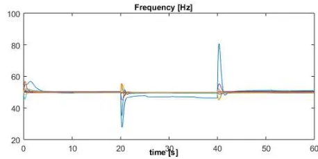
The plots below show the results of the simulation. Figures 9 and 10 show that the system still converges, but as expected, for some nodes the difference in magnitude of their responses is larger than in previous examples since an approximation to the real values was used. The power flow response does not fluctuate in magnitude and is always contained within 1 MWh from the reference value. In the frequency response there is a peak, which is motivated by a large connectivity of the node of City Road representing a source for all its neighbours. Hence this micro grid has to increase its frequency to provide sufficient power to all other nodes in order to steer all their responses from the initial state to the reference. Let us finally mention that in this set of simulations, the final value for every node is different. This is due to the heterogeneous nature of the oscillators which cannot reach frequency synchronization as long as the values are apart from each other within an acceptable range.

Fig. 9. Frequency response for the directed, weighted and approximated configuration.

Fig. 10. Power flow response for the directed, weighted and approximated configuration.

V. CONCLUSION

We have studied the transient stability, discussed the scal-ability of the model approach and provided an insight of the resilience of a network of interconnected micro grids. The findings have shed light on the capability of the micro grids to remain synchronised despite the heterogeneous and uncertain nature of the parameters characterizing the micro grids. Further direction of this work involves the analysis of the impact of stochastic disturbances due to renewable generation and demand response under on-line dynamic pricing.

ACKNOWLEDGEMENT

The first author would like to thank Mexico’s CONACyT for the support during his studies.

REFERENCES [1] F. Bullo.Lectures on Network Systems. 2016.

[2] R. Olfati Saber, J. A. Fax, and R. M. Murray. Consensus and Cooperation in Multi-Agent Networked Systems. Proceedings of IEEE, 95(1):215– 233, 2007.

[3] T. Namerikawa, N. Okubo, R. Sato, Y. Okawa, and M. Ono. Real-Time Pricing Mechanism for Electricity Market with Built-In Incentive for Participation. IEEE Transactions on Smart Grid, 6(6):2714–2724, 2015. [4] F. D¨orfler and F. Bullo. Synchronization and Transient Stability in Power Networks and Nonuniform Kuramoto Oscillators. SIAM Journal on Control and Optimization, 50(3):1616–1642, jan 2012.

[5] I. A. Hiskens. Introduction to Power Grid Operation.Ancillary Services from Flexible Loads CDC’13, 2013.

[6] UK Power Networks. Regional Development Plan City Road City of London (excluding 33kV). 2014.