Asynchronous circuit simulation and design methodologies

(1)

Rochester Institute of Technology

RIT Scholar Works

Theses

Thesis/Dissertation Collections

5-1-1999

Asynchronous circuit simulation and design

methodologies

Michael Hevery

Follow this and additional works at:

http://scholarworks.rit.edu/theses

This Thesis is brought to you for free and open access by the Thesis/Dissertation Collections at RIT Scholar Works. It has been accepted for inclusion

in Theses by an authorized administrator of RIT Scholar Works. For more information, please contact

[email protected]

.

Recommended Citation

(2)

ASYNCHRONOUS CIRCUIT

SIMULATION AND DESIGN

METHODOLOGIES

by

Michael Hevery

A thesis submitted

in

Partial Fulfillment of the

Requirements for the Degree of

MASTER OF SCIENCE

in

Computer Engineering

Approved by

Principal Advisor:

Dr. Kenneth W. Hsu, Professor

Committee

Member:

_

Dr. Tony H. Chang, Professor

Committee

Member:

_

Dr. Pawel Sniatala, Visiting Assistant Professor

Department of Computer Engineering

Kate Gleason College of Engineering

Rochester Institute of Technology

Rochester, New York

(3)

(4)

ABSTRACT

The

purpose

of

this

thesis

is

to

examine

asynchronous

design

as

a

possible

alternative

to

synchronous

design.

Asynchronous

design

promises

better

power

consumption

and

higher

performance.

In

this thesis

an asynchronous simulator capable of

predicting

asynchronous system

performance

is designed. The

simulator

is based

on a

probabilistic

event

driven

model

of

asynchronous elements.

The

simulator

is

performance

oriented

only,

and

thus

is

not

capable

of

functional

simulation

or

verification.

It

provides

a

highly

abstract view of

the

system.

Using

the

simulator

several

design

methodologies

were

inspected

and

simulated

for

their

performance.

Particular

attention

is

paid

to

differences

between

synchronous

and asynchronous

methodologies.

In

addition several

current

sensor

techniques

were examined

as

a possible

way

of

implementing

asynchronous

circuit completion

detection.

The

contribution of

this thesis

is definition

of

the

reasons

why

the

current

sensing

is

not a

feasible way for

completion

detection,

and

the

ability

to

predict

the

asynchronous

(5)

CONTENTS

CHAPTER

1

ASYNCHRONOUS CIRCUITS:

THE

PROMISED

LAND

1

1.1

Introduction

1

1.2

Benefits

of

Asynchronous

Circuits

2

1.2.1

Clock Distribution

2

1.2.2

Power Consumption

3

1.2.3

Faster Performance

4

1.2.4

Better Spectral Noise

4

1.3

Simulation

of

Asynchronous Systems

4

CHAPTER

2:EVENT

DRIVEN

SYSTEM MODEL

6

2.1

Clocked

Systems

6

2.2

Event

Driven Systems

6

2.3

Datagrams

7

2.4

Data

Flow Architecture

8

CHAPTER

3:ASYNSIM:

THE ASYNCHRONOUS SIMULATOR

9

3.1

Data

Flow Simulation

9

3.1.1

Performance

Simulation

9

3.1.2

Functional Simulator

10

3.1.3

Architectural Simulation

10

3.2

Architecture

10

3.3

Topology

11

3.3.1

Datagrams

11

3.3.2

Nodes

12

3.3.3

Paths

12

3.3.4

Probabilistic

Delay

Distribution

13

3.4

Request/ Acknowledge Communication Protocol

14

3.4.1

Datagram

Passing

75

3.4.2

Pipeline

(1:1)

15

3.4.3

Split

Pipeline

(1:2)

16

3.4.4

Merged

Pipeline

2:1

18

3.4.5

Cross

Over Pipeline

(2:2)

19

3.4.6

Path

Buffering

19

3.5

Topology

Description Language

20

3.5.1

Syntax

20

3.5.2

Node

22

3.5.3

Path

24

3.5.4

Delay

26

3.5.5

Token Initialization

28

3.5.6

Topology

example:

A Simple CPU

29

3.6

Output

30

3.6.1

Event Transcript

31

3.6.2

Path Status

33

3.6.3

Node Status

35

3.7

Simulating Synchronous Systems

36

CHAPTER

4:METHODS

OF IMPROVING ASYNCHRONOUS THROUGHPUT

37

4.1

Synchronous

vs.

Asynchronous

37

4.2

Pipelines

39

(6)

4.2.2

Asynchronous

40

4.2.3

Buffered Path

41

4.2.4

Dual Path

Buffering

42

CHAPTER

5:ASYNCHRONOUS

CIRCUIT

COMPLETION

DETECTION

BY

CURRENT

SENSING

44

5.1.1

Function Generation

44

5.1.2

Handshaking

Logic

45

5.2

Completion Signal Generation

by

Current

Sensing

45

5.2.1

Completion Detection

by

Current

Sensing

46

5.2.2

Probabilistic Distribution ofDelays

47

5.3

Measuring

the

Current Sensor

Quality

48

5.3.1

Voltage

Drop

48

5.3.2

Capacitance

49

5.3.3

Sensing Delay

49

5.3.4

Recovery

Time

49

5.3.5

Max Current

49

5.3.6

Voltage

Drop

per mA

49

5.3.7

Quiescent Current Consumption

49

5.4

Different Types

of

Current Sensing Circuits

50

5.4.1

Basic Current Sensors

50

5.4.2

DC

Analysis of Current Sensors

50

5.4.3

Current Sensor

with

Feedback

52

5.5

Current

and

Capacitance Distribution

53

5.5.7

Power

Consumption

53

5.5.2

Capacitor

/

Resistor

Network Distribution

54

5.5.3

Quiescent Current Consumption

56

5.5.4

Effects

of Gain Bandwidth Product

56

5.6

Time Delay Due

to

Long

SignalLines

57

CHAPTER

6:CONCLUSION

59

REFERENCES

60

APPENDIX

A:

ASYNSIM: SOURCE FTLES

/ SIMULATION

63

A.l.

Asynchronous Pipeline

64

A.7.7.

Topology

64

A.l.

2.

Simulation

65

A.l.

Asynchronous

Pipeline

with

Path

Buffering

67

A.2.1.

Topology

67

A.2.2.

Simulation

68

A.3.

Asynchronous Pipeline

with

Dual Path Buffering

69

A.J. 7.

Topology

69

A.3.2.

Simulation

70

APPENDK B: CURRENT SENSORS SCHEMATICS

72

(7)

(8)

LIST

OF

FIGURES

Figure 3.1: AsynSim

usage

model

11

Figure 3.2: Example

of a

node

with

paths

1 1

Figure 3.3: Example

of

a probabilistic

delay

distribution

13

Figure

3.4: Request /

Acknowledge

protocol

14

Figure 3.5: 1:1

pipeline configuration

16

Figure 3.6: 1

:2

split

path

configuration

17

Figure

3.7: 2:1 datagram

merge

path

18

Figure 3.8: 2:2 Cross

over

19

Figure 3.9: Path

buffering

20

Figure 3.10: Portion

of a

topology

file

declaring

three

paths

(A, B,

Sum)

and

a node

(ALU)

21

Figure 3.11:

Topology

file

describing

an

ALU

21

Figure 3.12: Node

attributes

23

Figure

3.13: Path

attributes

24

Figure 3.14: Simple

time

delay

26

Figure 3.15: Time

delay

range

27

Figure 3.16: Piecewise linear

delay

distribution

construction

27

Figure 3.17: Multilevel

piecewise

linear distribution

construction

27

Figure 3.18: Syntax for

absolute

token

initialization

28

Figure 3.19: Sequential

token

initialization

29

Figure 3.20: Simple CPU

topology

29

Figure 3.21: Simple CPU implemented

as an

AsynSim

topology

file

30

Figure 3.22: AsynSim

Even Transcript

results

31

Figure 3.23: Visual

time

representation

of

the

Event Transcript

results

32

Figure 3.24: Sample

path status

34

Figure 3.25:

Sample

node status

35

Figure 3.26: Asynchronous

pipeline

36

Figure

3.27: Modified

pipeline

to

support a

clock

36

Figure 4.1: Acknowledgment penalty

38

Figure 4.2:

Pipeline

representation

39

Figure 4.3:

Asynchronous

pipeline with

buffered

paths

41

Figure 4.4:

Asynchronous

pipeline with

dual

path

buffering

42

Figure 5.1: Function

generator

45

Figure 5.2:

Handshaking

logic

45

Figure

5.3:

Current

sensors

for

completion

detection

46

Figure 5.4:

Probabilistic

delay

distribution

of

functional

block

47

Figure

5.5: Current

sensors

based

on

(a)

Comparator

(b)

BJT

(c)

Current

mirror

50

Figure 5.6: Voltage

vs. current

DC

response of current sensors

51

Figure 5.7:

Current

sensor with

feedback

52

Figure 5.8:

Voltage

versus current

DC

response of an active current sensor

52

Figure 5.9:

Minimal switching

current consumption configuration

53

(9)

Figure 5.11:

(a)

Transistor

schematic

(b)

Power distribution

net

(c)

Simplified

54

(10)

LIST

OF TABLES

Table 4.1: Pipeline

parameters

39

Table 4.2: Performance summary for

an asynchronous pipeline

40

an asynchronous pipeline with path

buffering

42

an

asynchronous pipeline with

dual

path

buffering.

43

(11)

GLOSSARY

Asynchronous

page

2

A

clockless

design methodology

that

employs

handshaking

protocols

to

control

the

flow

of

data.

AsynSim

page

9

Asynchronous Simulator developed for

this

thesis.

Datagram

page

7

A

package of

data

and state

information

that

is

passed

between

nodes

Node

page

12

A functional block

that

computes a

new

datagram

on

its

output(s)

after

consuming

the

datagrams

on

its input(s).

Path

page

12

Communication

route

for datagrams.

Synchronous

page

6

(12)

Chapter

1:

Asynchronous

Circuits: The

Promised

Land

1.1 Introduction

In

recent

years

the

semiconductor

industry

has

managed

to

consistently improve

the

performance

of

its

products.

These improvements have

come

in

two

categories:

the

semiconductor

process;

and

the

novel architectural

design

of

digital logic. Semiconductor

process

improvements

allow

the

shrinking

of

transistors

which permits

an

increased

number

of

transistors

on

the

same

area

of

silicon.

These

improvements

allow

the

architectural

designers

greater

freedom

and

allow

for designs

of

higher

complexity.

However,

increasing

the

number

of

transistors

on a

chip

creates new challenges

that

will

have

to

be

overcome

in

new

designs. Two

of

these

challenges

are

power

consumption

and clock

distribution. Each

will need

to

be

solved

in

order

to

move

to

the

(13)

1.2

Benefits

of

Asynchronous

Circuits

One

technology

that

is promising

to

solve

the

dual

problems of clock

distribution

and power

dissipation

is

asynchronous

circuit

design.

1.2.1

Clock Distribution

Asynchronous

design

eliminates

clocks.

The

elimination

of

a

clock within a

system

both

solves and creates

new problems.

In

current

synchronous

designs

a

centralized

clock

is

responsible

for

synchronizing

all

events.

The

synchronization

of

events

greatly

simplifies

design

and

makes

it

more predictable.

Unfortunately

it

also

creates problems

of

clock

distribution,

power consumption and clock

skew.

A

clocked system needs

to

constantly

charge and

discharge

the

clock

distribution

network.

Because

this

network needs

to trace to

every

flip-flop

or

latch in

the

system

it is

inherently

large

and

therefore

has

a

large

capacitance.

Constant charging

and

discharging

of

the

clock

distribution

network

creates

heavy

currents

and

therefore

consumes

significant

power.

The

constant

presence

of

the

clock signal

is

inefficient,

because

not all

units

in

a system need

the

clock

at

all

times.

For

example

clocking

the

floating-point

unit

(FPU)

in

a processor

is unnecessary

unless

the

processor

is currently performing

floating

point

arithmetic.

However,

even

if

a processor

can

disable

the

clock

to

some of

its

units,

as

many

modern processors

do,

it

can

only do

so at a coarse

level. No design

can control

which

register

receives

a

clock

and

when,

such

a

fine

control

would

be

inefficient.

Therefore

at

best

the

current modern

designs

can

group

blocks

together

(14)

In

addition

to

power

consumption,

clocked systems

face

the

problem of clock

skew.

Having

a

large,

capacitive network

requires

time

for

a clock edge

to

propagate

to

all

parts of

the

chip.

This

propagation

delay

is

small,

however

as

the

clock speed

reaching

1 GHz

the

percentage of

the

whole clock

cycle which

is

taken

up

by

the

clock skew

is

becoming

significant.

Having

a

large

percentage of

the

clock cycle occupied

by

clock

skew

degrades

the

performance of

the

system.

Asynchronous

systems

attempt

to

solve

these

problems

by

the

elimination of

the

clock altogether

from

the

system.

Since

clock signals need

to travel to

all parts

of

the

chip, the

clock

period

is limited

by

the

propagation

delay

of

the

clock

network.

In

asynchronous

design

no such

limitation

exists.

In

addition,

in

asynchronous

systems,

signals

are

time

independent from

all other signals

within a system.

This is

not

true

in

clocked

systems since

all

signals

are

dependent

and must arrive at

their

destination before

the

clock.

1.2.2 Power

Consumption

Asynchronous

systems promise

to

be

more

power efficient.

Their efficiency is

mainly due

to

a

lack

of constant

charging

and

discharging

of

the

clock

network.

In

addition,

asynchronous circuits are event

driven

and consume power

only if

an event

needs

to

be

processed.

If

there

is

no event

to

be

processed asynchronous circuits will

stay

idle

consuming leakage

current only.

On

the

other

hand

synchronous circuits perform

"null"

(15)

1.2.3 Faster Performance

In

a

synchronous

system

the

clock

period

must

accommodate

the

worst

case

scenario.

Most

circuits

within

a

system will

perform

better

and

finish

within

the

clock

period

most

of

the time.

In

addition

the

worst case

delay

might

be

rare,

for

example

it

might occur

in

the

processor

only if

a

certain

instruction is

executed.

If

such

an

instruction

is

rare

the

system

is

underutilized

most of

the time

and could

be running

at a

higher

frequency. Asynchronous

systems

do

not

suffer

from

these

limitations

since each

element within

the

system runs at

its

own pace.

1.2.4 Better

Spectral

Noise

Finally,

asynchronous circuits

offer

better

spectral

noise.

Synchronous

systems

have

a spectral noise with

a

large

peak

at

the

clock

frequency. On

the

other

hand

the

noise

in

the

asynchronous system

is

more even

across

all

frequencies,

this

is mostly due

to

lack

of centralized control.

[15]

1.3

Simulation

of

Asynchronous

Systems

To

further investigate

the

above

claims

of performance

gain

a

"Performance

Simulator"

was

designed

with asynchronous circuits

in

mind.

This

was named

AsynSim

(Asynchronous

Simulator)

and

attempts

to

predict

the

performance

of

a

system

by

simulating

the

flow

of

data

through

it. AsynSim is

not a

functional

simulator,

and

thus

can not

predict

the

correctness of

the

model.

In

addition

AsynSim

is

a

very

high

level

(16)

system's

behavior before its

implementation.

The

simulator

is based

on an event

driven

(17)

Chapter

2:

Event Driven System

Model

An

event

driven

system model

is

the

basis for

the

asynchronous

system.

It is

sometimesreferred

to

as a

data flow

model or

data flow

architecture.

2.1 Clocked

Systems

In

synchronous systems

the

clock

is

the

driving

force.

During

each clock cycle

the

state of

the

system

is known

precisely.

In

fact

the

current

state can

be defined

as

the

current

value

of all

latches

as

well as

the

current values

of

all

inputs. Given

a set

of

known

values

for

the

inputs

and

for

the

latches

there

exist

only

one

Such

systems

are well

behaved,

because

each clock period creates a well-defined

state.

The

state

machines

in

synchronous systems

take

advantage

of

this

property

and use

it

to

direct

the

flow

of

data

through the

system.

2.2 Event

Driven Systems

Event driven

systems on

the

other

hand do

not need a

well-defined state.

In fact

a

(18)

Instead in

an event

driven

system

each

functional

unit

has its

own

state,

such

as

busy,

or

ready.

This

state

defines

whether

the

unit

is

able

to

accept

new

input

events.

The

current

state

of an event

driven

system

is defined

by

the

location

of

the

events within

the

system.

The

advantage

of such

a

system

is

that

it only

performs

actions

if

there

is

something

to

do

and

therefore

only

consumes

power

as

needed.

In

addition

an event

driven

system

is

localized,

since

it only depends

on

the

delays

of

its inputs

and outputs

and

not

on

the

delay

of

the

whole system.

2.3

Datagrams

In

event

driven

systems

the

event refers

to the

presence

of a

new

datagram

on

the

unit's

input. The

unit

consumes

the

datagram

package

compromising

several

different

individual data

elements.

For

example

an

ALU performing

addition

has

a

datagram

consisting

of

A

operand,

B

operand and an

addition

directive. In

addition

a

datagram

might

contain

routing

information

directing

the

result

of

the

addition.

Routing

information is necessary because

event

driven

systems

lack

a

global

state

that

would

otherwise

direct

the

output of

the

data. Instead

the

data

needs

to

be

able

to

route

itself. A

datagram

together

with

its location

within

the

system

represent

the

current state.

Datagram

methodology

is very different from

synchronous

design

methodology

which

usually

has

control and

data

separated.

In

asynchronous systems

this

separation

is

(19)

2.4 Data

Flow

Architecture

There

has been

a

lot

of

research

done in

the

are of

data flow

architectures.

Two

of

which are

Petri

nets and

the

data flow

architecture

for

parallel

programming

as

developed

by

MIT

[13]. Data flow

architectures

have

the

advantage of

being

decentralized,

which

is

exactly

what an asynchronous system needs.

Data flow

architectures

transfer

control

to

the

data

and

its location

within

the

system

rather

than to

a

centralized

set

of

state

(20)

Chapter

3:

AsynSim: The

Asynchronous

Simulator

The

idea behind

the

simulator

is

to

allow

a

performance

analysis

of an

asynchronous

system

design. The

simulator consists of a set of nodes and a set of paths

that

interconnect

the

nodes.

The

performance

is

obtained

by

measuring

the

time

it

takes

for

the

system

to

process

a

set

of

tokens.

During

the

processing

of

the tokens the

simulator

takes

into

account

the

delays in

the

paths as well as

the

delays in

the

nodes.

3.1

Data

Flow Simulation

Data flow

simulation

as

presented

in AsynSim

allows

only

a

very high level

simulation

for

use

early in

the

design

process.

AsynSim

is

a probabilistic

simulator;

therefore

its

output

is

non-deterministic.

The

power of

the

simulation

is in running

large

token

sets which produce a statistical model of

the

system's performance.

3.1.1

Performance Simulation

The

data flow

simulation allows

the

designer

to

see

the

performance of

the

system

(21)

expected

timing

delays

of

the

functional

units specifies

the

probabilities.

The

simulation

is

not

highly

accurate

prediction

of

how

the

system will

behave

rather

it is

an average

prediction

how

the

system will

behave

most of

the time

given

the

probabilities supplied.

3.1.2 Functional Simulator

The

simulator

is

not

a

functional

simulator since

the

description

of

the

system

is

of

the

highest

level

possible.

Functional

simulation

on

the

other

hand

requires a

highly

detail description. The

idea

of

high level

simulation

is

to

perform simulations

early in

the

design

process

and

to

see

how

the

data

flow

will

behave

before

designing

the

functionality

of

any

of

the

individual

nodes.

3.1.3 Architectural Simulation

The

simulator

does

allow

the

verification

of

an

architecture.

It

allows

the

verification

of

deadlock

avoidance.

It

can also show which

nodes

are

over or

under

utilized

and

thus

aid

in redesigning

the

system

to

redistribute

the

data flow.

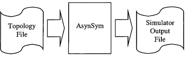
3.2 Architecture

The

AsynSim

overall

usage

model

is

shown

in Figure 3.1. It

consists

of

a

topology

file

which

describes

the

system under simulation

as

the

set of

nodes, paths,

their

interconnections

and a stimulus.

Based

on

the

topology

file AsynSim

then

produces an

(22)

Topology

File

AsynSym

Simulator

Output

File

Figure

3.1: AsynSim

usage model.

3.3

Topology

The

topology

file describes

the

system under simulation.

For

example

in Figure

3.2

an asynchronous adder

is

shown.

It

consists

of

two

inputs A

and

B

and an output

Sum. In AsynSim topology, processing

elements

are called

nodes

and

connections

between

nodes are called

paths.

Therefore Figure 3.2 has

three

paths

(A, B,

Sum)

and one

node

(ALU).

Figure

3.2: Example

of a node with paths.

3.3.1

Datagrams

are

packages

of

data,

its

state,

and

any

other

information

that

is

[image:22.571.78.389.91.189.2]

(23)

generated on

the

output

of

a

node

it

creates an event

for

that

path.

Similarly

when

the

datagram

arrives

at

the

end

of

a path

it

creates

an

event

for

the

destination

node

to

process

it. Datagram

movements

are

responsible

for

events and

the

events

they

produce

is

what

drives

the

system.

Datagrams

observe

the

delays

of nodes and paths as

they

travel

through

the

system.

In AsynSim

the

datagram's location is

represented

by

a

token.

3.3.2 Nodes

A

node

in AsynSim

represents

a

processing

element.

A

node

has

one or more

inputs

and

one or more outputs.

In

addition a node

has

some

delay

associated with

it.

When

a

datagram

arrives

on

the

node's

input

and generates an

event,

the

node checks

if

all of

its inputs have

a

datagram

waiting.

If

all

inputs have datagrams waiting

and

the

node

is

free,

then the

node

consumes

all

of

the

datagrams

at

once

and

proceeds

to

calculate a new output

datagram

some

delay

later. Once

the

output

datagram is

generated

it

then

is

passed

to the

appropriate output.

The

output

is

a

function

of

the

datagrams just

processed.

The

node remains

in

the

busy

state

until

the

path

at

the

output acknowledges

the

receipt

of

the

datagram.

3.3.3

Paths

are

responsible

for moving datagrams

around

the

system.

They

are

the

delivery

mechanism

by

which

the

system communicates.

As

this

is

an

asynchronous

system

the

paths must also contain

the

handshaking

protocol.

Each

path

has

a

delay

associated with

it

representing

the

time

it

takes

for

the

(24)

datagram,

the

path

is

responsible

for acknowledging

to the

source node

that

the

datagram

has

been

passed on

successfully.

3.3.4

Probabilistic

Delay

Distribution

To

better

approximate

the

delays in

asynchronous

systems, the

delays

in AsynSim

have

a probabilistic

distribution

as shown

Figure 3.3.

2.0

4.0

6.0

Time

(ns)

8.0

Figure 3.3: Example

of a probabilistic

delay

distribution.

In

the

example

in Figure 3.3

the

delay

is

never more

then

8ns

or

less

than

2ns,

while

most

of

the time the

delay

is

around

4ns. These kinds

of

dynamic delays

can

better

approximate

what will

happen in

an

asynchronous system.

For

example a ripple

carry

adder might

have

a

very

long

worst case

delay

which occurs when

adding

two

numbers

that

will

cause

the

ripple

carry

to

propagate

through

all of

the

bits. Such

cases

however,

are

rare.

It is

more probable

that

only

a

few

bits

will generate a

carry

out and

the

carry

out

(25)

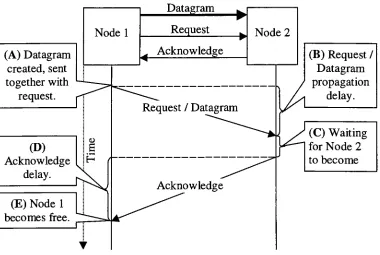
3.4 Request /

Acknowledge

Communication Protocol

When

the

nodes

are

communicating

with each

other

they

must

follow

an

established protocol

to

ensure

that

no

data is lost in

the

transmission.

The

protocol

followed in

asynchronous systems

is

the

request

/

acknowledge protocol.

Datagram

(A)

Datagram

created,

sent

together

with

request.

(D)

Acknowledge

delay.

(E)

Node 1

becomes

free.

(B)

Request /

Datagram

propagation

delay.

(C)

Waiting

for Node 2

to

become

[image:25.571.76.456.189.444.2]

Figure

3.4:

Request /

Acknowledge

protocol.

Figure 3.4

shows an

interaction

between

two

nodes

and

how

one

datagram flows

from Node 1

to

Node 2. In

the

upper part

of

the

Figure 3.4

a physical

interconnection is

shown.

Node 1

has

data

lines

shown

by

the thick

arrow

connecting it

to

node

2. Node 1

also

has

a request

line connecting it

to

Node

2. Node 2 has

an

acknowledge

signal

connecting it

back

to

Node 1.

The

lower

part of

Figure 3.4

shows a

time

representation of

the

event exchange.

First

Node 1

generates a

datagram

and asserts

the

request

line

as

shown

in (A). The

(26)

later

they

reach

Node 2

as

shown

in (B). This

delay

is known

as request

delay

within

the

AsynSim.

Once

the

request

arrives at

Node

2,

Node 2 may

or

may

not

respond

immediately

with an

acknowledgement.

The

delay

in

(C)

is dependent

on

what

state

Node 2 is

in.

If Node 2 is free

then the

response

is

immediate,

if

on

the

other

hand Node 2

is in

the

middle of

calculating

a

datagram

or

is itself waiting for

an acknowledgement

the

delay

in

(C)

might

be longer. At

some

point

Node 2

becomes free

and consumes

the

datagram

produced

by

Node 1

at which

point

it

notifies

Node 1

by

the

acknowledgement

shown

in (C). The

acknowledgement

has

to traverse the

return

path

to

Node 1

and

is

delayed

as shown

in (D).

Finally

as

Node 1

receives

the

acknowledgment

it becomes free

and

stops

driving

the

datagram lines. The

process

described

above

is known

as

the

Request

/ Acknowledge Communication Protocol

and

is

used

in AsynSim.

3.4.1 Datagram

Passing

AsynSim follows

the

Request / Acknowledge Communication Protocol in its

simulations

of an

asynchronous

system.

AsynSim

allows

the

designer

to

define

the

request

and acknowledge

delay. In

addition

there

are a

few

other parameters which effect

the

communication path which

handle

all

of

the

requests and acknowledgements.

Nodes

are

only

responsible

for

the

consumption and generation

of

datagrams

within

the

system.

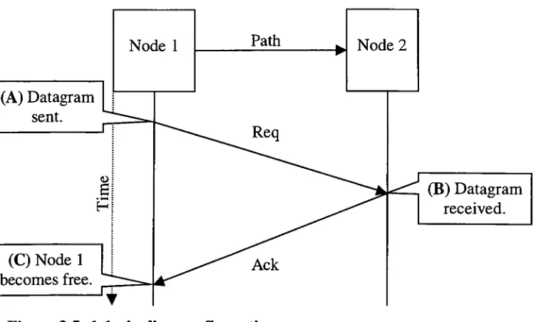
3.4.2

Pipeline

(1:1)

A

pipeline

is

the

simplest case of a

data

path.

It

involves

a connection

between

(27)

(A)

Datagram

sent.

Nodel

(C)

Node

1

becomes

free.

Path

Node 2

(B)

Datagram

received.

[image:27.571.80.456.60.286.2]

Figure

3.5: 1:1

pipeline configuration.

Figure 3.5

shows

the

simplest configuration

that

AsynSim

supports.

A

one

to

one

configuration

is

created

between

the

sender

and receiver.

AsynSim handles

this

as

a

simple

request

/

acknowledge

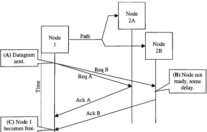
communication.

3.4.3 Split

Pipeline

(1:2)

AsynSim

also supports a

data

path

that

has

more

than

one

destination.

A

split

configuration

is

created

when

a single

node's

output

is

connected

to

more

than

one

(28)

(A)

Datagram

sent.

(C)

Node

1

becomes

free.

Node

2B

(B)

Node

not

ready,

some [image:28.571.72.491.56.324.2]

delay.

Figure 3.6: 1:2

split path configuration.

Figure

3.6

shows a single source

node with

two

destination

nodes.

To

make

the

transition

more

interesting

assume

that

Node 2A is

initially

free

and

Node 2B is

initially

busy. When

the

request arrives

at

Node

2A,

because Node 2A is free it is

able

to

respond

immediately

with

an

acknowledgment,

while

Node 2B

requires

more

time

before it

becomes free

and

thus

incurs

some

delay

as

shown

in (B). Node 1 does

not

become free

until

it

gets

an acknowledgement

from

all of

the

nodes as shown

in (C).

There

exists an alternate mode of

operation,

in

which

the

originating

node waits

for only

one acknowledgment and

only

one

request

is

delivered,

to

the

first

node

that

is

free. This

second mode of operation

is known

as

First Free

Delivery

and

is

useful

in

situations

where

two

nodes

can

perform

the

same

operations

on

a

datagram

and

to

increase

performance

they

are arranged

in

parallel.

For

example

a

CPU

might

have

two

(29)

twice

and would

keep

both

of

the

floating-point

units

busy. Instead

the

first free

floating

point

unit

gets

the

datagram. This

allows

for

parallel

processing

of

data

with can

improve

overall

throughput.

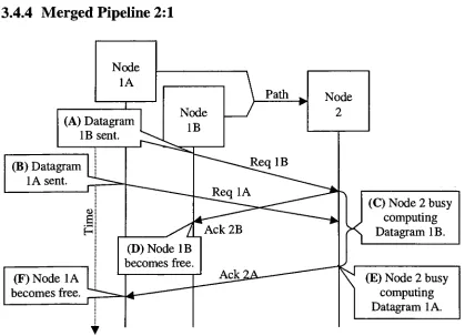
3.4.4

Merged Pipeline

2:1

Node

1A

(A)

Datagram

IB

sent.

(B)

Datagram

1A

sent.

(F)

Node

1A

becomes

free.

(D)

Node IB

becomes free.

(C)

Node

2

busy

computing

Datagram IB.

(E)

Node 2

busy

computing

Datagram 1A.

Figure

3.7:

2:1

datagram

merge path.

It is

possible

for

two

nodes

to talk

to the

same

destination

node.

In

such a case

the

datagrams

need

to

be

synchronized

to

form

a single

sequential

input

to

Node 2. AsynSim

supports

this

model and grants

the

acknowledgment

to the

first datagram

that

arrived.

After Node 2

has

processed

the

first datagram it

can process

the

second at which point

the

[image:29.571.69.488.157.460.2]

(30)

3.4.5

Cross Over

Pipeline

(2:2)

A

cross

over

allows

multiple

sources

to talk

to

multiple

destinations.

In

this

configuration

either each

datagram is delivered

to

each

destination

node or

the

First Free

Delivery

model

can

be

adopted.

Node

1A

\

Path

/

Node

2

^

Node

IB

Node

2

w

Figure

3.8: 2:2 Cross

over.

The

acknowledgement and

request paths of

the

2:2

cross over

follow

those

of

the

2:1

and

1:2

examples,

or

are simplified when

First Free

Delivery

is

used.

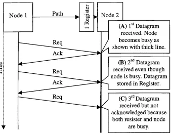
3.4.6 Path

Buffering

Finally

a

special

feature

of

AsynSim

allows

a

buffered

path.

A buffered

path

consists

of

one

or

more registers

before

the

destination

node.

This

register can

latch

the

datagram

and send an acknowledgement

to the

source node even

if

the

destination

node

is

(31)

(A)

Is

Datagram

received.

Node

becomes

busy

as

shown with

thick

line.

,nd

(B)

2

Datagram

received even

though

node

is busy. Datagram

stored

in Register.

(C)

3rd

Datagram

received

but

not

acknowledged

because

both

resister and node

are

busy.

Figure

3.9: Path buffering.

Path

buffering

allows

better

performance

because

datagrams

can

be

acknowledged

faster

and

the time

source nodes

spend

waiting for

acknowledgements can

be

minimized.

More

about

path

buffering

in

Chapter

4:

Methods

of

Improving

Asynchronous

Throughput.

3.5

Topology

Description

Language

AsynSim

uses a

description language

similar

to

C

to

describe

all

nodes, paths,

and

their

interconnections.

It

also

describes

the

delays

within

the

system.

3.5.1

Syntax

The

language is very flexible

and should allow a

description

of almost all system

[image:31.571.78.416.58.323.2]

(32)

before

on object can

be further described. This

prevents one

from accidentally

creating

new objects

by

the

misspelling

of an

object's

name.

After

the

object

declaration

the

object's

details

are

described. These details include

delays,

connections

and

special

behavior if

any.

An

example of an

AsynSim

topology

file

with

declarations

is

shown

below.

//

Double

slash

is

a comment.

//

Path

command

lists

all of

the

paths

in

the

system

//

Notice

the

ft-'

on

the

end of

the

line.

Path{A,

B,

Sum

};

//

Similarly

Node

command

declares

node(s)

.

Node

{ALU};

Figure

3.10: Portion

of a

topology

file

declaring

three

paths

(A, B,

Sum)

and a

node

(ALU).

A

sample

ALU is built in Figure 3.2. The ALU

node

and

its

paths

have been

declared

and now

the

interconnections

need

to

be defined

as

shown

in Figure 3.11.

//

ALU

(Graphic

is

a

comment)

.

//

-A->|

\

//

>

ALU

|

-Sum-->

//

-B->|

/

//

Declare

the

paths

Path

(A,

B,

Sum

}

;

//

Declare

the

node

Node

{ALU};

//

Define

the

interconnections.

ALU{

in

=

{A,

B},

out =

Sum

};

(33)

Figure

3.11

represents one of

the

smallest

topology

files

that

will

successfully

pass

through

AsynSim.

Of

course

this

file

will not simulate

anything

but it describes

a

topology

and shows

the

organization of a sample

topology

file.

3.5.2 Node

A

node

is

a

functional

unit of

an asynchronous

design. A

node can

be in

one of

the

three

states.

1)

Initially

the

node

is free

to

perform

calculations.

In

the

free

state

the

node

has

no

pending input datagrams

and

is ready

to

start

processing

as

soon as all of

its inputs

are

ready.

2)

Once

all

of

the

inputs have

a

datagram

present

the

node enters

the

busy

state.

In

the

busy

state

the

node

is computing

the

result.

This

is

the

only

time

when

the

node

is

being

productive.

A

good

design

will

attempt

to

keep

the

node

in

the

busy

state

as

much

as possible.

3)

Finally,

after

the

node computes

the

resulting datagram it

places

it

on

the

output and

enters a

waiting

state.

In

the

waiting

state

the

node

is

not

doing

anything,

just like in

free

state,

but

unlike

the

free

state

the

node

is

not

allowed

to

accept

inputs. This is

because

the

newly

created

datagram has

not

been

accepted

yet

and

if

a

new

calculation were started

this

datagram

would

be

overwritten.

A

good

design

tries to

minimize

the

waiting

state since a node needs

to

be kept

productive.

In

addition

a

node

can

have

several

other

attributes

that

further

describe

its

behavior.

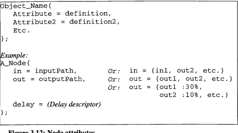
Each

attribute

has

an equal sign and a

definition

as shown

Figure 3.12. The

delay

descriptor is

more complicated and

is

explained

in

more

detail later

in

section

3.5.4

(34)

Object_Name{

Attribute

=

definition,

Attribute2

=

def

inition2

,

Etc.

};

Example:

A_Node

{

in

=

input Path,

Or:

in

==

{inl,

_out

2

,

etc.}

out = _output

Path,

Or:

_out =

{outl,

out2

,

etc.}

Or:

out =

{outl

:30%,

out2

:10%,

etc.}

delay

-(Delay

descriptor)

};

Figure

3.12: Node

attributes.

Below

are

the

definitions

and

the

functionality

of all of

the

attributes

that the

node

declaration

accepts.

3.5.2.1

in

The in

attribute

defines

all of

the

inputs

of

the

node.

If

there

is

more

than

one

input, they

can

be

enclosed

in curly braces.

3.5.2.2

out

The

out

attribute

defines

all of

the

outputs of

the

node.

If

there

is

more

than

one

output,

they

can

be

enclosed

in curly braces. The

output

datagram from

a node

can

be

assigned

to

one output only.

By

default if

more

than

one

output

exists

the

datagrams

generated

are

assigned

in

a

round

robin

fashion. If

a

random

assignment

scheme

is

desired

then

each output can

be

qualified

with

a percentage probability.

In

that

case

the

datagrams

are

assigned

at

random

in

accordance

with

the

probabilities

specified.

If

[image:34.571.71.465.62.283.2]

(35)

3.5.2.3

delay

The

delay

attribute specifies

the

delay

from

the time

the

datagram

is

consumed

by

the

node

until a new

datagram is

generated on

the

node's output.

It

represents

the

node

delay

and

is

specified with a

delay

descriptor,

the

syntax

for

which

is

explained

in

section

3.5.4

Delay.

3.5.3 Path

A

path

is

responsible

for moving

the

datagrams

from

the

source

node

to the

destination

node.

The

request

and

acknowledgement

delays define

the

communication

speed.

After

a

node

generates

a

datagram

the

path's

destination

node

is

notified of

the

request

some

delay

later. If

the

destination

node

is free

to

accept

a

datagram

then

it

consumes

the

datagram

and sends an

acknowledge

signal

back

to the

originating

node.

Once

that

node receives

the

acknowledgment after

some

delay

it is free

to

generate

a new

datagram.

The remaining

attributes

further define

path

behavior.

Object_Name{

Attribute

==

definition,

Attribute2

=

def

inition2

,

Etc.

};

Example:

A_Path{

req

=

delay,

ack =

delay,

token

=

token_

initialization,

queueDepth

=

depth,

delivery

=

/anylall/

};

[image:35.571.69.468.433.647.2]

(36)

3.5.3.1

req

The

req

attribute

defines

a

delay

between

the

creation of

the

datagram

in

the

node

and

its

arrival

at

the

destination

node.

This

time

delay

is usually

defined

as

the

transmission

delay

of

the

path

between

two

nodes.

3.5.3.2

ack

The

ack

attribute

defines

a

delay

from

the time the

datagram is

consumed

by

the

destination

node

until

the

path

delivers

the

acknowledgement

back

to the

originating

node.

3.5.3.3 token

The

token

attribute allows

the

paths

to

be initialized

with

datagrams for

simulation.

For further

explanation and

syntax refer

to

section

3.5.4

3.5.3.4

queueDepth

The

queueDepth

attribute

defines

the

number of

buffering

registers

for

datagrams in

the

path.

Usually

the

path

does

not

have

registers

associated with

it. It is

possible

for

a

path

to

have

a

simple

register

to

latch

a

datagram

and

thus

free

the

originating

node

even

if

the

destination

node

is

not

ready

to

a consume

the

datagram.

By

default

the

queueDepth

is 0

and

therefore the

path acts

as

a

simple

transmission

line.

There

is

also a special value of

infinity

which

creates an

infinite

number of

buffering

elements.

3.5.3.5

delivery

The

delivery

attribute

defines

how

the

path

behaves if

there

is

more

than

one

(37)

path receives one

copy

of

the

datagram.

That

is in

the

1:2

configuration

the

two

destination

nodes

both

get a

copy

of

the

datagram

and must

acknowledge

it before

the

source node

can proceed with

processing its

However,

specifying

the

any

attribute

for

delivery

tells the

simulator

to

assign

the

datagram

to the

first

available

destination

(First Free Destination). This

is

useful

when

the two

destination

nodes

are

identical

and

both

can process

the

datagram

in

the

same way.

For

example

a

CPU

having

two

floating-point

units where

the

first floating-point

unit

to

become free

can process

the

datagram.

3.5.4

Delay

In

AsynSim

the

delays

are

not

fixed,

rather

they

have

a probabilistic

distribution.

The

syntax

for

defining

the

distribution

is based

on a

tree

configuration

with each

node

having

a

delay

range and a continuous

probability distribution.

The

simplest

form

of

delay

is

a

constant

time

as

in Figure 3.14. Notice

the

'ns'

following

the time.

The AsynSim

understands

following

list

of

suffixes:

sec, ms, us,

ns, ps,

f

s.

3

ns

Figure

3.14: Simple

time delay.

It

is

also

possible

to

define

ranges

of

time

as

show

in Figure 3.15. Note

the

distinction

between

square

bracket

'['

and

parenthesis

')'. A

square

bracket

implies

that

the

associated

end point of

the

specified

time

is

included in

the range,

while a parenthesis

implies

that

its

associated end point

is

excluded

from

the time

range.

From

the

example

in

Figure 3.15

the

AsynSim

will

randomly

generate numbers

from

3ns (inclusive

to

less

(38)

[3

ns,

5ns)

//

space optional

Figure 3.15: Time

delay

range.

It is

also

possible

to

construct

any

delay

distribution from

a piecewise

linear

summation of

many

smaller ranges as shown

in Figure 3.16. A

percentage

that

specifies

the

likelihood

of a number within

that

range

being

chosen

follows

each

linear

range.

Please

note

that

all percentages must add

up

to

100% for

each

delay

distribution.

{

[3

ns,

5ns)

:20%,

[5

ns,

6.5ns)

:80%

Figure

3.16: Piecewise linear

delay

distribution

construction.

Finally,

piecewise

linear

delay

construction can

have

multiple

levels

of

delay

ranges

as

shown

in Figure 3.17. In

the

first level

the

delay

is divided into

a

20%

probability from 3

ns

to

5

ns

and

an

80% probability in

two

ranges

with

their

own

percentages.

Notice

that the

outer percentages

add

up

to

100% (20%

+

80%)

and

the

second

level

percentages also add

up

to

100% (40%

+

60%). Of

course

there

is

no

limit

to

how many levels

a

delay

definition

can

have.

{

[3

ns,

5ns)

:20%,

{

[5

ns,

4ns)

:40%,

[4

ns,

6.5ns)

:60%,

}:80%

Figure

3.17:

Multilevel

piecewise

linear

distribution

construction.

Using

combinations

of

many

small

linear

regions

any

delay

distribution

can

be

(39)

3.5.5

Token Initialization

When simulating

a

design in AsynSim it is necessary

to

introduce

datagrams into

system

at specific

times to

simulate

the throughput

of

the

system.

In AsynSim datagrams

are

called

tokens.

The difference between

tokens

and

datagrams is

that

a

datagram

carries

data

to

be

processed,

while

token

is just

a

placeholder.

AsynSim is

not

a

functional

simulator

and

therefore

does

not perform

any kind

of operations on

the

data (in fact data

is

absent

from

the

simulations),

instead

the

focus is

on

how

fast

these

datagrams

move

through the

system.

Therefore in

place

of

datagrams AsynSim

uses

tokens.

Token

initialization

comes

in

two

forms. Absolute

initialization is

a

list

of

tokens

to

be inserted

at

the

given specific

times.

The

other

form is

of sequential

token

streams.

An

example

of

absolute

initialization

is

shown

in Figure 3.18. First

at

3ns

tokenl

is introduced into

the

system.

Then

somewhere

between 4ns

and

5ns

a

second

token

token2

will

be introduced. Notice

that time

specifications

are

in

the

delay

notation

introduced in 3.5.2.3 delay.

{

name

@

delay,

name

@

delay,

etc.

}

Example:

{

tokenl

@

3ns,

token2

@

[4ns,

5ns]

}

Figure

3.18: Syntax for

absolute

token

initialization.

Initialization

of

tokens

as a

sequential

stream

is

shown

in

Figure

3.19. Note

the

(40)

in Figure

3.19

will

generate

tokens

fast_l,

f

ast_2,

etc.

at a rate of

2ns. At

the

same

time

slow_l, slow_2,

etc.

is

generated at a rate of

15

to

25ns.

{

}

name

[from,

to]

every

delay,

name

(from,

to)

every

delay,

etc. . .

Example:

{

fast

[1,100]

every

2ns,

slow

(0,10]

every

[15ns,

25ns]

}

Figure

3.19: Sequential

token

initialization.

3.5.6

Topology

example:

A

Simple CPU

To

better

explain

how

the

individual

parts of

AsynSim

work

together

a simple

CPU design is

shown

in Figure 3.20.

Instruction

fetch:

85%: hit 5ns

15%:

miss

15ns

Op.

queue:

Depth 5 inst.

Req/Ack:

Ins

20%: l-2ns

20%

:

2-5ns

50%: 5-1 Ons

10-50ns

Memory

Queue depth:

infinite

Result

queue:

Depth 5

results

Req/Ack

Ins

Write back:

85%: hit 5ns

15%:

miss

15ns

Figure

3.20: Simple CPU

topology.

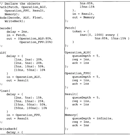
The

CPU

of

Figure 3.20 is

represented

in

AsynSim

topology

language

in

Figure

(41)

//

Declare

the

objects

5ns:85%,

Path

{Fetch,

Operation_ALU,

15ns: 15%

Operation_FPU,

Result,

},

Memory}

;

in

=

Result,

Node

{Decode,

ALU,

Float,

out =

Memory

WriteBack}

;

};

Decode

{

Fetch

{

delay

=

2ns,

token

=

{

in

=

Fetch,

lnst[0,

1000]

every

{

out =

{Operation_ALU:80%,

5ns:85%,

15ns:15%

}

Operation_FPU

:

2 0%

}

};

}

};

ALU{

Operation_ALU

{

delay

=

{

queueDepth =

5,

[Ins,

2ns)

:

20%,

req

=

Ins,

[2ns,

5ns)

:

20%,

ack =

Ins

[5ns,

10ns)

:

50%,

};

[10ns,

50ns]

:

10%

}

Operation_FPU{

in

=

Operation_ALU,

queueDepth =

5,

out =

Result

req

=

Ins,

};

ack =

Ins

};

Float

{

delay

=

{

Result

{

[2ns,

5ns)

:

15%,

queueDepth =

5,

[5ns,

15ns)

:

25%,

req

=

Ins,

[15ns,

50ns)

:

50%,

ack =

Ins

[50ns,

100ns]

:

10%

}

in

=

Operation_FPU,

};

Memory {

out =

Result

_queueDepth =

infinite.

};

req

-

Ins,

ack =

Ins

WriteBack

{

};

delay

=

{

Figure

3.21:

Simple CPU

implemented

as an

AsynSim

topology

file.

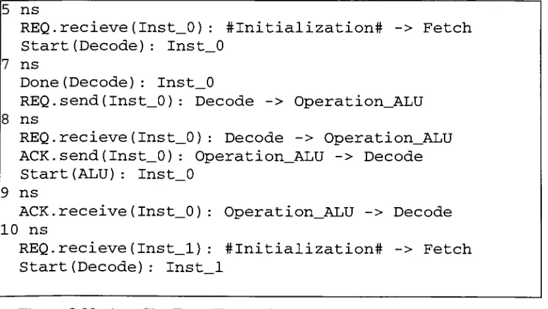
3.6 Output

After

executing

a

topology

file,

AsynSim

returns

the

simulation

results.

The

simulation

results are

divided

into

three

categories.

The Event

Transcript

shows all of

the

[image:41.571.74.493.60.498.2]

(42)

shows

which

paths

have

tokens

waiting in

them.

And

finally

Node Status

shows

the

utilization

of

the

nodes.

These

results give