Quadratic differentials as stability conditions

White Rose Research Online URL for this paper:

http://eprints.whiterose.ac.uk/84399/

Version: Accepted Version

Article:

Bridgeland, T. and Smith, I. (2014) Quadratic differentials as stability conditions.

Publications mathématiques de l'IHÉS. ISSN 0073-8301

https://doi.org/10.1007/s10240-014-0066-5

[email protected] https://eprints.whiterose.ac.uk/ Reuse

Unless indicated otherwise, fulltext items are protected by copyright with all rights reserved. The copyright exception in section 29 of the Copyright, Designs and Patents Act 1988 allows the making of a single copy solely for the purpose of non-commercial research or private study within the limits of fair dealing. The publisher or other rights-holder may allow further reproduction and re-use of this version - refer to the White Rose Research Online record for this item. Where records identify the publisher as the copyright holder, users can verify any specific terms of use on the publisher’s website.

Takedown

If you consider content in White Rose Research Online to be in breach of UK law, please notify us by

TOM BRIDGELAND AND IVAN SMITH

Abstract. We prove that moduli spaces of meromorphic quadratic differentials with simple zeroes on compact Riemann surfaces can be identified with spaces of stability conditions on a class of CY3triangulated categories defined using quivers with

poten-tial associated to triangulated surfaces. We relate the finite-length trajectories of such quadratic differentials to the stable objects of the corresponding stability condition.

Contents

1. Introduction 1

2. Quadratic differentials 13

3. Trajectories and geodesics 22

4. Period co-ordinates 33

5. Stratification by number of separating trajectories 42

6. Colliding zeroes and poles: the spaces Quad(S,M) 56

7. Quivers and stability conditions 65

8. Surfaces and triangulations 75

9. The category associated to a surface 85

10. From differentials to stability conditions 94

11. Proofs of the main results 100

12. Examples 113

References 122

1.

Introduction

In this paper we prove that spaces of stability conditions on a certain class of

tri-angulated categories can be identified with moduli spaces of meromorphic quadratic

differentials. The relevant categories are Calabi-Yau of dimension three (CY

), and are

described using quivers with potential associated to triangulated surfaces. The

observa-tion that spaces of abelian and quadratic differentials have similar properties to spaces

of stability conditions was first made by Kontsevich and Seidel several years ago. On

the one hand, our results provide some of the first descriptions of spaces of stability

conditions on CY

categories, which is the case of most interest in physics. On the

other, they give a precise link between the trajectory structure of flat surfaces and the

theory of wall-crossing and Donaldson-Thomas invariants.

Our results can also be viewed as a first step towards a mathematical understanding

of the work of physicists Gaiotto, Moore and Neitzke [13, 14]. Their paper [13]

de-scribes a remarkable interpretation of the Kontsevich-Soibelman wall-crossing formula

for Donaldson-Thomas invariants in terms of hyperk¨ahler geometry. In the sequel [14]

an extended example is described, relating to parabolic Higgs bundles of rank two. The

mathematical objects studied in the present paper are very closely related to their

phys-ical counterparts in [14], and some of our basic constructions are taken directly from

that paper. We hope to return to the relations with Hitchin systems and cluster

vari-eties in a future publication. In another direction, the CY

categories appearing in this

paper also arise as Fukaya categories of certain quasi-projective Calabi-Yau threefolds.

That relation is the subject of a sequel paper [35].

In this introductory section we shall first recall some basic facts about quadratic

differ-entials on Riemann surfaces. We then describe the simplest examples of the categories

we shall be studying, before giving a summary of our main result in that case, together

with a very brief sketch of how it is proved. We then state the other version of our result

involving quadratic differentials with higher-order poles. We conclude by discussing the

relationship between the finite-length trajectories of a quadratic differential and the

stable objects of the corresponding stability condition.

As a matter of notation, the triangulated categories we consider here are most

natu-rally labelled by combinatorial data consisting of a smooth surface

S

equipped with a

collection of marked points

M

_⊂

S

, all considered up to diffeomorphism. Initially

S

will be closed, but in the second form of our result

S

can have non-empty boundary.

The quadratic differentials we consider live on Riemann surfaces

S

whose underlying

smooth surface is obtained from

S

by collapsing each boundary component to a point.

To avoid confusion, we shall try to preserve the notational distinction whereby

S

refers

to a smooth surface, possibly with boundary, whereas

S

is always a Riemann surface,

usually compact. All these surfaces will be assumed to be connected.

We fix an algebraically closed field

k

throughout.

1.1.

Quadratic differentials.

A meromorphic quadratic differential

φ

on a Riemann

surface

S

is a meromorphic section of the holomorphic line bundle

ω

. We

empha-size that all the differentials considered in this paper will be assumed to have simple

zeroes. Two quadratic differentials

φ

, φ

on Riemann surfaces

S

, S

are considered to

be equivalent if there is a holomorphic isomorphism

f

:

S

→

S

such that

f

(

φ

) =

φ

.

Let

S

be a compact, closed, oriented surface, with a non-empty set of marked points

By a quadratic differential on (

S

,

M

) we shall mean a pair (

S, φ

), where

S

is a compact

and connected Riemann surface of genus

g

=

g

(

S

), and

φ

is a meromorphic quadratic

differential with simple zeroes and exactly

d

=

_|

M

_|

poles, each one of order

6

2. Note

that every equivalence class of such differentials contains pairs (

S, φ

) such that

S

is the

underlying smooth surface of

S

, and

φ

has poles precisely at the points of

M

.

A quadratic differential (

S, φ

) of this form determines a double cover

π

: ˆ

S

_→

S

, called

the spectral cover, branched precisely at the zeroes and simple poles of

φ

. This cover

has the property that

π

(

φ

) =

ψ

_⊗

ψ

for some globally-defined meromorphic 1-form

ψ

. We write ˆ

S

_⊂

_S

ˆ

_{for the complement}

of the poles of

ψ

. The hat-homology group of the differential (

S, φ

) is defined to be

ˆ

H

(

φ

) =

H

( ˆ

S

;

Z

)

where the superscript indicates the anti-invariant part for the action of the covering

involution. The 1-form

ψ

is holomorphic on ˆ

S

_{and anti-invariant, and hence defines a}

de Rham cohomology class, called the period of

φ

, which we choose to view as a group

homomorphism

Z

: ˆ

H

(

φ

)

→

C

,

γ

7→

Z

γ

ψ.

There is a complex orbifold Quad(

S

,

M

) of dimension

n

= 6

g

₋

6 + 3

d

parameterizing equivalence-classes of quadratic differentials on (

S

,

M

). We call a

qua-dratic differential complete if it has no simple poles; such differentials form a dense open

subset Quad(

S

,

M

)

⊂

Quad(

S

,

M

).

The homology groups ˆ

H

(

φ

) form a local system over the orbifold Quad(

S

,

M

)

. A

slightly subtle point is that this local system does not extend over Quad(

S

,

M

), but

rather has monodromy of order 2 around each component of the divisor

parameteriz-ing differentials with a simple pole. It therefore defines a local system on an orbifold

Quad

(

S

,

M

) which has larger automorphism groups along this divisor. There is a

natural map

Quad

(

S

,

M

)

_→

Quad(

S

,

M

)

,

which is an isomorphism over the open subset Quad(

S

,

M

)

, and which induces an

isomorphism on coarse moduli spaces. Fixing a free abelian group Γ of rank

n

, we can

also consider an unramified cover

Quad

(

S

,

M

)

_−→

Quad

(

S

,

M

)

In Section 4 we shall prove the following result, which is a variation on the usual

existence of period co-ordinates in spaces of quadratic differentials. For this we need to

assume that (

S

,

M

) is not a torus with a single marked point.

Theorem 1.1.

The space of framed differentials

Quad

(

S

,

M

)

is a complex manifold,

and there is a local homeomorphism

(1.1)

π

: Quad

(

S

,

M

)

_−→

Hom

(Γ

,

C

)

,

obtained by composing the framing and the period.

In the excluded case the space Quad

(

S

,

M

) is not a manifold because it has generic

automorphism group

Z

.

1.2.

Triangulations and quivers.

Suppose again that

S

is a compact, closed, oriented

surface with a non-empty set of marked points

M

_⊂

S

. For the purposes of the following

discussion we will assume that if

g

(

S

) = 0 then

_|

M

_|

>

5.

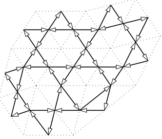
By a non-degenerate ideal triangulation of (

S

,

M

) we mean a triangulation of

S

whose

vertex set is precisely

M

and in which every vertex has valency at least 3. To each such

triangulation

T

there is an associated quiver

Q

(

T

) whose vertices are the midpoints of

the edges of

T

, and whose arrows are obtained by inscribing a small clockwise 3-cycle

inside each face of

T

, as illustrated in Figure 1.

Figure 1.

Quiver associated to a triangulation.

There are two obvious systems of cycles in

Q

(

T

), namely a clockwise 3-cycle

T

(

f

) in

each face

f

, and an anticlockwise cycle

C

(

p

) of length at least 3 encircling each point

p

_∈

M

. We define a potential

W

(

T

) on

Q

(

T

) by taking the sum

W

(

T

) =

X

f

T

(

f

)

₋

X

p

Consider the derived category of the complete Ginzburg algebra [15, 23] of the quiver

with potential (

Q

(

T

)

, W

(

T

)) over

k

, and let

_D

(

T

) be the full subcategory consisting of

modules with finite-dimensional cohomology. It is a CY

triangulated category of finite

type over

k

, and comes equipped with a canonical t-structure, whose heart

_A

(

T

)

_{⊂ D}

(

T

)

is equivalent to the category of finite-dimensional modules for the completed Jacobi

algebra of (

Q

(

T

)

, W

(

T

)).

Suppose that two non-degenerate ideal triangulations

T

are related by a flip, in which

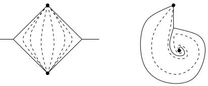
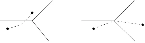
the diagonal of a quadilateral is replaced by its opposite diagonal, as in Figure 2. The

point of the above definition is that the resulting quivers with potential (

Q

(

T

)

, W

(

T

))

are related by a mutation at the vertex corresponding to the edge being flipped; see

Fig-ure 2. It follows from general results of Keller and Yang [23] that there is a distinguished

pair of

k

-linear triangulated equivalences Φ

:

D

(

T

)

∼

=

D

(

T

).

Figure 2.

Effect of a flip.

Labardini-Fragoso [27] extended the correspondence between ideal triangulations and

quivers with potential so as to encompass a larger class of triangulations containing

vertices of valency

6

2. He then proved the much more difficult result that flips induce

mutations in this more general context. Since any two ideal triangulations are related

by a finite chain of flips, it follows that up to

k

-linear triangulated equivalence, the

category

_D

(

T

) is independent of the chosen triangulation. We loosely use the notation

D

(

S

,

M

) to denote any triangulated category

_D

(

T

) defined by an ideal triangulation

T

of the marked surface (

S

,

M

).

1.3.

Stability conditions.

A stability condition on a triangulated category

_D

is a

pair

σ

= (

Z,

_P

) consisting of a group homomorphism

Z

:

K

(

_D

)

_→

C

called the central

charge, and an

R

-graded collection of objects

P

=

[

φ∈R

P

(

φ

)

_{⊂ D}

known as the semistable objects, which together satisfy some axioms (see Section 7.5).

For simplicity, let us assume that the Grothendieck group

K

(

_D

) is free of some finite

rank

n

. There is then a complex manifold Stab(

_D

) of dimension

n

whose points are

stability conditions on

_D

satisfying a further condition known as the support property.

The map

taking a stability condition to its central charge is a local homeomorphism. The manifold

Stab(

_D

) carries a natural action of the group Aut(

_D

) of triangulated autoequivalences

of

_D

.

Now suppose that (

S

,

M

) is a compact, closed, oriented surface with marked points, and

let

_D

be the CY

triangulated category

D

(

S

,

M

) defined in the last subsection. There

is a distinguished connected component

Stab

(

D

)

⊂

Stab(

D

)

,

containing stability conditions whose heart is one of the standard hearts

_A

(

T

)

_{⊂ D}

(

T

)

discussed above. We write

Aut

(

D

)

⊂

Aut(

D

)

for the subgroup of autoequivalences of

_D

which preserve this component. We also

define

Aut

(

D

) to be the quotient of Aut

(

D

) by the subgroup of autoequivalences

which act trivially on Stab

(

D

).

The first form of our main result is

Theorem 1.2.

Let

(

S

,

M

)

be a compact, closed, oriented surface with marked points.

Assume that one of the following two conditions holds

(a)

g

(

S

) = 0

and

_|

M

_|

>

5

;

(b)

g

(

S

)

>

0

and

_|

M

_|

>

1

.

Then there is an isomorphism of complex orbifolds

Quad

(

S

,

M

)

∼

= Stab

(

D

)

/

Aut

(

D

)

.

The assumption on the number of punctures in the

g

(

S

) = 0 case of Theorem 1.2 comes

from a similar restriction in a crucial result of Labardini-Fragoso [29]. We conjecture

that the conclusion of the Theorem holds with the weaker assumptions that

_|

M

_|

>

1

and that if

g

(

S

) = 0 then

_|

M

_|

>

3. The case of a once-punctured surface is special in

many respects, and we leave it for future research; see Section 11.6 for more comments

on this. The case of a three-punctured sphere is also special, and is treated in Section

12.4.

Away from its critical points (zeroes and poles), a quadratic differential

φ

on a Riemann

surface

S

induces a flat metric, together with a foliation known as the horizontal

folia-tion. One way to see this is to write

φ

=

dz

_{for some local co-ordinate}

_z

_{, well-defined}

up to

z

_{7→ ±}

z

+constant. The metric is then given by pulling back the Euclidean metric

on

C

using

z

, and the horizontal foliation is given by the lines Im(

z

) = constant.

The integral curves of the horizontal foliation are called trajectories. The trajectory

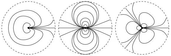
structure near a simple zero and a generic double pole are illustrated in Figure 3. Note

Figure 3.

Local trajectory structure at a simple zero and a generic

dou-ble pole.

that generic double poles behave like black holes: any trajectory passing beyond a

certain event horizon eventually falls into the pole. Thus for a generic differential one

expects all trajectories to tend towards a double pole in at least one direction.

In the flat metric on

S

induced by

φ

, any pole of order

>

2 lies at infinity. Therefore,

assuming that

S

is compact, any finite-length trajectory

γ

is either a simple closed curve

containing no critical points of

φ

, or is a simple arc which tends to a finite critical point

of

φ

(a zero or simple pole) at either end. In the first case

γ

is called a closed trajectory,

and moves in an annulus of such trajectories known as a ring domain. In the second

case we call

γ

a saddle trajectory. Note that the endpoints of a saddle trajectory

γ

could well coincide; when this happens we call

γ

a closed sadddle trajectory.

The boundary of a ring domain has two components, and each boundary component

usually consists of unions of saddle trajectories. There is one other possibility however: a

ring domain may consist of closed curves encircling a double pole

p

with real residue; the

point

p

is then one of the boundary components. We call such ring domains degenerate.

There is a dense open subset

B

⊂

Quad(

S

,

M

) consisting of differentials (

S, φ

) with

no simple poles and no finite-length trajectories; we call such differentials saddle-free.

For saddle-free differentials, each of the three horizontal trajectories leaving a given

zero eventually tend towards a double pole. These separating trajectories divide the

surface

S

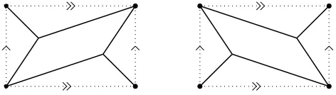
into a union of cells, known as horizontal strips (see Figure 5). Taking a

Figure 5.

The separating (solid) and generic trajectories (dotted) for a

saddle-free differential; the black dots represent double poles.

single generic trajectory from each horizontal strip gives a triangulation of the surface

S

, whose vertices lie at the poles of

φ

, and this then induces an ideal triangulation

T

of the surface (

S

,

M

), well-defined up to the action of the mapping class group. This is

what is referred to as the WKB triangulation in [14].

The dual graph to the collection of separating trajectories is precisely the quiver

Q

(

T

)

considered before. In particular, the vertices of

Q

(

T

) naturally correspond to the

hori-zontal strips of

φ

. In each horizontal strip

h

there is a unique homotopy class of arcs

ℓ

joining the two zeroes of

φ

lying on its boundary. Lifting

ℓ

to the spectral cover gives a

class

α

∈

H

ˆ

(

φ

), and taken together, these classes form a basis. There is thus a natural

isomorphism

ν

:

K

(

_D

(

T

))

_→

H

ˆ

(

φ

)

,

which sends the class of the simple module

S

at a vertex of

Q

(

T

), to the class

α

defined

by the corresponding horizontal strip

h

.

Using the isomorphism

ν

, the period of

φ

can be interpreted as a group homomorphism

Z

:

K

(

D

(

T

))

→

C

. More concretely, this is given by

Z

(

S

) = 2

Z

ℓi

p

φ

_∈

C

,

where the sign of

√

φ

is chosen so that Im

Z

(

S

)

>

0. We thus have a triangulated

category

_D

(

T

), with its canonical heart

_A

(

T

), and a compatible central charge

Z

. This

We refer to the connected components of the open subset

B

as chambers; the horizontal

strip decomposition and the triangulation

T

are constant in each chamber, although

the period

Z

varies. As one moves from one chamber to a neighbouring one, the

triangulation

T

can undergo a flip. Gluing the stability conditions obtained from all

these chambers using the Keller-Yang equivalences Φ

referred to above eventually leads

to a proof of Theorem 1.2.

1.5.

Higher-order poles.

We can extend Theorem 1.2 to cover quadratic differentials

with poles of order

>

2. Such differentials correspond to stability conditions on

cate-gories defined by triangulations of surfaces with boundary. For this reason it will be

convenient to also index the relevant moduli spaces of differentials by such surfaces, as

we now explain.

A marked, bordered surface (

S

,

M

) is a pair consisting of a compact, oriented, smooth

surface

S

, possibly with boundary, together with a collection of marked points

M

_⊂

S

,

such that every boundary component of

S

contains at least one point of

M

. The marked

points

P

_⊂

M

lying in the interior of

S

are called punctures. We shall always assume

that (

S

,

M

) is not one of the following:

(i) a sphere with

6

2 punctures;

(ii) an unpunctured disc with

6

2 marked points on its boundary.

These excluded surfaces have no ideal triangulations, and so our theory would be

vac-uous in these cases.

The trajectory structure of a quadratic differential

φ

near a higher-order pole is

illus-trated in Figure 6; just as with double poles there is an event horizon beyond which

all trajectories tend to the pole, but at a pole of order

k

+ 2 there are, in addition,

k

distinguished tangent vectors along which all trajectories enter.

Figure 6.

Local trajectory structure at a pole of order 5.

A meromorphic quadratic differential

φ

on a compact Riemann surface

S

determines a

marked, bordered surface (

S

,

M

) by the following construction. To define the surface

considered as points of the interior of

S

, together with the points on the boundary of

S

corresponding to the distinguished tangent directions.

Let us now fix a marked, bordered surface (

S

,

M

). Let Quad(

S

,

M

) denote the space

of equivalence classes of pairs (

S, φ

), consisting of a compact Riemann surface

S

,

to-gether with a meromorphic quadratic differential

φ

with simple zeroes, whose associated

marked bordered surface is diffeomorphic to (

S

,

M

).

More concretely, the pair (

S

,

M

) is determined up to diffeomorphism by the genus

g

=

g

(

S

), the number of punctures

p

=

_|

P

_|

, and a collection of integers

k

>

1 encoding

the number of marked points on each boundary component of

S

. The space Quad(

S

,

M

)

then consists of equivalence classes of pairs (

S, φ

) consisting of a meromorphic quadratic

differential

φ

on a compact Riemann surface

S

of genus

g

, having

p

poles of order

6

2,

a collection of higher-order poles with multiplicities

k

+ 2, and simple zeroes.

The space Quad(

S

,

M

) is a complex orbifold of dimension

n

= 6

g

₋

6 + 3

p

+

X

i

(

k

+ 3)

.

We can define the spectral cover

π

: ˆ

S

_→

S

, the hat-homology group ˆ

H

(

φ

), and the

spaces Quad

(

S

,

M

) and Quad

(

S

,

M

) exactly as before. We can also prove the analogue

of Theorem 1.1 in this more general setting.

The theory of ideal triangulations of marked bordered surfaces has been developed

for example in [10]. The results of Labardini-Fragoso [27] apply equally well in this

more general situation, so exactly as before, there is a CY

triangulated category

D

=

_D

(

S

,

M

), well-defined up to

k

-linear equivalence, and a distinguished connected

component Stab

(

D

).

The second form of our main result is

Theorem 1.3.

Let

(

S

,

M

)

be a marked bordered surface with non-empty boundary. Then

there is an isomorphism of complex orbifolds

Quad

(

S

,

M

)

∼

= Stab

(

D

)

/

Aut

(

D

)

.

There are six degenerate cases which have been suppressed in the statement of Theorem

1.3. Firstly, if (

S

,

M

) is one of the following three surfaces

(a) a once-punctured disc with 2 or 4 marked points on the boundary;

(b) a twice-punctured disc with 2 marked points on the boundary;

then Theorem 1.3 continues to hold, but only if we replace

Aut

(

D

) by a certain index

surface is not determined up to the action of the mapping class group by the associated

quiver

Q

(

T

). Secondly, if (

S

,

M

) is one of the following three surfaces

(c) an unpunctured disc with 3 or 4 marked points on the boundary;

(d) an annulus with one marked point on each boundary component;

then the space Quad(

S

,

M

) has a generic automorphism group which must first be killed

to make Theorem 1.3 hold. These exceptional cases are treated in more detail in Section

11.6.

Particular choices of the data (

S

,

M

) lead to quivers of interest in representation theory.

See Section 12 for some examples of this. In particular, we can recover in this way some

recent results of T. Sutherland [37, 38], who used different methods to compute the

spaces of numerical stability conditions on the categories

_D

(

S

,

M

) in all cases in which

these spaces are two-dimensional.

1.6.

Saddle trajectories and stable objects.

In the course of proving the Theorems

stated above, we will in fact prove a stronger result, which gives a direct correspondence

between the finite-length trajectories of a quadratic differential and the stable objects

of the corresponding stability condition.

To describe this correspondence in more detail, fix a marked bordered surface (

S

,

M

)

satisfying the assumptions of one of our main theorems, and let

_D

=

_D

(

S

,

M

) be

the corresponding triangulated category. Let

φ

be a meromorphic differential on a

compact Riemann surface

S

defining a point

φ

_∈

Quad(

S

,

M

), and let

σ

_∈

Stab

(

D

)

be the corresponding stability condition, well-defined up to the action of the group

Aut

(

D

). We shall say that the differential

φ

is generic if for any two hat-homology

classes

γ

∈

H

ˆ

(

φ

)

R

_·

Z

(

γ

) =

R

·

Z

(

γ

) =

⇒

Z

·

γ

=

Z

·

γ

.

Generic differentials form a dense subset of Quad(

S

,

M

), and for simplicity we shall

restrict our attention to these.

To state the result, let us denote by

_M

(0) the moduli space of objects in

D

that are

stable in the stability condition

σ

and of phase 0. This space can be identified with

a moduli space of stable representations of a finite-dimensional algebra, and hence by

work of King [24], is represented by a quasi-projective scheme over

k

.

Theorem 1.4.

Assume that

φ

is generic. Then

_M

(0)

is smooth, and each of its

con-nected components is either a point, or is isomorphic to the projective line

P

. Moreover,

there are bijections

0-dimensional components of

_M

(0)

←→

non-closed saddle trajectories of

φ

;

1-dimensional components of

_M

(0)

←→

Note that with our conventions, all trajectories are assumed to be horizontal, and

correspond to stable objects of phase 0. In particular, a stability condition

σ

has a

stable object of phase 0 precisely if the corresponding differential

φ

has a finite-length

trajectory. Stable objects of more general phases

θ

correspond in exactly the same way

to finite-length straight arcs which meet the horizontal foliation at a constant angle

πθ

. This more general statement follows immediately from Theorem 1.4, because the

isomorphisms of our main theorems are compatible with the natural

C

-actions on both

sides.

Standard results in Donaldson-Thomas theory imply that the two types of moduli spaces

appearing in Theorem 11.6 contribute +1 and

₋

2 respectively to the BPS invariants,

although we do not include the proof of this here. These exactly match the

contri-butions to the BPS invariants described in [14, Section 7.6]. In physics terminology,

non-closed saddle trajectories correspond to BPS hypermultiplets, and non-degenerate

ring domains to BPS vectormultiplets.

It is a standard open question in the theory of flat surfaces to characterise or constrain

the hat-homology classes which contain saddle connections. Theorem 1.4 relates this to

the similar problem of identifying the classes in the Grothendieck group which support

stable objects. Here one has the powerful technology of Donaldson-Thomas invariants

and the Kontsevich-Soibelman wall-crossing formula [26], which in principle allows one

to determine how the spectrum of stable objects changes as the stability condition

varies. It would be interesting to see whether these techniques can be usefully applied

to the theory of flat surfaces.

1.7.

Structure of the paper.

The paper splits naturally into three parts.

The first part, consisting of Sections 2–6, is concerned with spaces of meromorphic

qua-dratic differentials. Section 2 reviews basic notions concerning quaqua-dratic differentials,

and introduces orbifolds Quad(

g, m

) parameterizing differentials with simple zeroes and

fixed pole orders. Section 3 consists of well-known material on the trajectory structure

of quadratic differentials. Section 4 is devoted to proving that the period map on

Quad(

g, m

) is a local isomorphism. Section 5 studies the stratification of the space

Quad(

g, m

) by the number of separating trajectories. Finally, Section 6 introduces the

spaces Quad(

S

,

M

) appearing above, in which zeroes of the differentials are allowed to

collide with the double poles.

The second part, comprising Sections 7–9, is concerned with CY

triangulated

The geometry and algebra come together in the last part, which comprises Sections 10–

12. Section 10 describes the WKB triangulation associated to a saddle-free differential,

and the way it changes as one passes between neighbouring chambers. Section 11

contains the proofs of our main results identifying spaces of stability conditions with

spaces of quadratic differentials. We finish in Section 12 with some illustrative examples.

The reader is advised to start with

_§§

2–3, the first half of

_§

6, and

_§§

7–9, since these

contain the essential definitions and are the least technical. It may also help to look at

some of the examples in

_§

12.

Acknowledgements.

Thanks most of all to Daniel Labardini-Fragoso, Andy Neitzke and

Tom Sutherland, all of whom have been enormously helpful. Thanks too to Sergey

Fomin, Bernhard Keller, Alastair King, Howard Masur, Michael Shapiro and Anton

Zorich for helpful conversations and correspondence. This paper owes a significant debt

to the work of Davide Gaiotto, Greg Moore and Andy Neitzke [14].

2.

Quadratic differentials

We begin by summarizing some of the basic properties of meromorphic quadratic

dif-ferentials on Riemann surfaces. This material is mostly well-known, although we were

unable to find any references dealing with the moduli spaces of differentials with

higher-order poles that we shall be using. Our standard reference for quadratic differentials is

Strebel’s book [36].

2.1.

Quadratic differentials.

Let

S

be a Riemann surface, and let

ω

denote its

holomorphic cotangent bundle. A

meromorphic quadratic differential

φ

on

S

is a

mero-morphic section of the line bundle

ω

. Two such differentials

φ

, φ

on surfaces

S

, S

are said to be equivalent if there is a biholomorphism

f

:

S

→

S

such that

f

(

φ

) =

φ

.

In terms of a local co-ordinate

z

on

S

we can write a quadratic differential

φ

as

φ

(

z

) =

ϕ

(

z

)

dz

_⊗

dz

with

ϕ

(

z

) a meromorphic function. We write Zer(

φ

)

,

Pol(

φ

)

_⊂

S

for the subsets of

zeroes and poles of

φ

respectively. The subset Crit(

φ

) = Zer(

φ

)

_∪

Pol(

φ

) is the set of

critical points

of

φ

.

At a point of

S

_\

Crit(

φ

) there is a distinguished local co-ordinate

w

, uniquely defined

up to transformations of the form

w

_{7→ ±}

w

+ constant, with respect to which

φ

(

w

) =

dw

_⊗

dw.

In terms of an arbitrary local co-ordinate

z

we have

w

=

R p

A quadratic differential

φ

determines two structures on

S

_\

Crit(

φ

), namely a flat metric

(called the

φ

-metric) and a foliation (the horizontal foliation). The

φ

-metric is defined

locally by pulling back the Euclidean metric on

C

using a distinguished co-ordinate

w

.

The horizontal foliation is given in terms of a distinguished co-ordinate by the lines

Im(

w

) = constant.

The

φ

-metric and the horizontal foliation on

S

_\

Crit(

φ

) together determine both the

complex structure on

S

and the differential

φ

. Note that the set of quadratic differentials

on a fixed surface

S

has a natural

S

_{-action given by scalar multiplication :}

_φ

_7→

_e

_·

_φ

_.

This action has no effect on the

φ

-metric, but alters which in the circle of foliations

defined by Im(

w/e

_{) = constant is regarded as being horizontal.}

In terms of a local co-ordinate

z

on

S

, the length of a smooth path

γ

in the

φ

-metric is

(2.1)

ℓ

(

γ

) =

Z

γ

|

ϕ

(

z

)

_|

_|

dz

_|

.

It is important to divide the critical set into a disjoint union

Crit(

φ

) = Crit

(

φ

)

∪

Crit

(

φ

)

,

where Crit

(

φ

) consists of

finite critical points

, namely zeroes and simple poles, and

Crit

(

φ

) consists of

infinite critical points

, that is poles of order

>

2. We write

S

₌

_S

_\

_Crit

∞

(

φ

)

for the complement of the infinite critical points.

Note that the integral (2.1) is well-defined for curves passing through points of Crit

(

φ

).

This gives the surface

S

_{the structure of a metric space, in which the distance between}

two points

p, q

_∈

S

_{is the infimum of the lengths of smooth curves in}

_S

_connecting

_p

to

q

. The topology on

S

_{defined by this metric agrees with the standard one induced}

from the surface

S

.

2.2.

GMN differentials.

All the quadratic differentials considered in this paper live

on compact surfaces and have simple zeroes and at least one pole. Since it will be

convenient to eliminate certain degenerate situations we make the following definition.

Definition 2.1.

A GMN differential is a meromorphic quadratic differential

φ

on a

compact, connected Riemann surface

S

such that

(a)

φ

has simple zeroes,

(b)

φ

has at least one pole,

(c)

φ

has at least one finite critical point.

Given a GMN differential (

S, φ

) we write

g

for the genus of the surface

S

and

d

for

the number of poles of

φ

. The

polar type

of

φ

is the unordered collection of

d

integers

m

=

_{

m

}

giving the orders of the poles of

φ

. We define

(2.2)

n

= 6

g

₋

6 +

d

X

i=1

(

m

+ 1)

,

A GMN differential (

S, φ

) is said to be

complete

if

φ

has no simple poles, or in other

words, if all

m

>

2. This is exactly the case in which the

φ

-metric on

S

\

Pol(

φ

) is

complete. At the opposite extreme, the differential (

S, φ

) is said to have

finite area

if

φ

has only simple poles, that is if all

m

= 1.

2.3.

Spectral cover and periods.

Suppose that

φ

is a GMN differential on a compact

Riemann surface

S

, with poles of order

m

at points

p

∈

S

. We can alternatively view

φ

as a holomorphic section

(2.3)

ϕ

_∈

H

(

S, ω

(

E

)

)

,

E

=

X

i

l

m

i

2

m

·

p

,

with simple zeroes at both the zeroes and the odd order poles of

φ

. The

spectral cover

of

S

defined by

φ

is the compact Riemann surface

ˆ

S

=

(

p, l

(

p

)) :

p

_∈

S, l

(

p

)

_∈

L

such that

l

(

p

)

⊗

l

(

p

) =

ϕ

(

p

)

⊂

L,

where

L

is the total space of the line bundle

ω

(

E

). This is a manifold because

ϕ

has

simple zeroes.

The obvious projection map

π

: ˆ

S

_→

S

is a double cover, branched precisely over the

zeroes and the odd order poles of the original meromorphic differential

φ

. There is a

covering involution

τ

: ˆ

S

_→

S

ˆ

, commuting with the map

π

. The surface ˆ

S

is connected

because Definition 2.1 implies that

π

has at least one branch point.

We define the hat-homology group of the differential

φ

to be

ˆ

H

(

φ

) =

H

( ˆ

S

;

Z

)

,

where ˆ

S

₌

_π

₍

_S

_{), and the superscript denotes the anti-invariant part for the action}

of the covering involution

τ

.

Lemma 2.2.

The group

H

ˆ

(

φ

)

is free of rank

n

given by

(2.2)

.

Proof. The Riemann-Hurwitz formula applied to the spectral cover

π

: ˆ

S

_→

S

implies

that

(2.4)

2ˆ

g

₋

2 = 2(2

g

₋

2) + (4

g

₋

4 +

d

X

i=1

m

) + (

d

−

e

)

,

where ˆ

g

is the genus of ˆ

S

, and

e

is the number of even

m

. The group

H

(

S

;

Z

) is

free of rank 2

g

+

d

₋

s

₋

1, where

s

is the number of simple poles. Similarly, using

equation (2.4), and noting that each even order pole has two inverse images in ˆ

S

, the

group

H

( ˆ

S

;

Z

) is free of rank

r

= 2ˆ

g

+

d

+

e

₋

s

₋

1 = 8

g

₋

6 +

d

X

i=1

m

+ 2

d

−

s

−

1

.

Since the invariant part of

H

( ˆ

S

;

Z

) can be identified with

H

(

S

;

Z

), the anti-invariant

part

H

( ˆ

S

;

Z

)

is therefore free of rank

n

.

The spectral cover ˆ

S

comes equipped with a tautological section

ψ

of the line bundle

π

₍

_ω

S

(

E

)) satisfying

π

(

ϕ

) =

ψ

⊗

ψ

and

τ

(

ψ

) =

−

ψ

. There is a canonical map

η

:

π

₍

_ω

S

)

→

ω

and we can form the composition

O

−−→

π

(

ω

(

E

))

−−−−→

ω

( ˆ

E

)

,

where ˆ

E

=

π

₍

_E

_{). This defines a meromorphic 1-form on ˆ}

_S

_{, which we also denote by}

ψ

.

Since the canonical map

η

vanishes at the branch-points of

π

, the differential

ψ

is regular

at the inverse images of the simple poles of

φ

, and hence restricts to a holomorphic

1-form on the open subsurface ˆ

S

_{. By construction}

_ψ

_{is anti-invariant for the action of}

the covering involution

τ

, and therefore defines a de Rham cohomology class

[

ψ

]

_∈

H

_{( ˆ}

_S

_;

_C

₎

called the period of

φ

. We choose to view this instead as a group homomorphism

Z

: ˆ

H

(

φ

)

→

C

.

2.4.

Intersection forms.

Consider a GMN differential

φ

on a Riemann surface

S

, and

its spectral cover

π

: ˆ

S

_→

S

. Write

ˆ

D

=

π

(Crit

(

φ

))

.

Thus ˆ

S

_{= ˆ}

_S

_\

_D

_ˆ

∞

. There are canonical maps of homology groups

H

( ˆ

S

;

Z

) =

H

( ˆ

S

\

D

ˆ

;

Z

)

−−→

H

( ˆ

S

;

Z

)

−−→

H

( ˆ

S,

D

ˆ

;

Z

)

.

The intersection form on

H

( ˆ

S

;

Z

) is a non-degenerate, skew-symmetric pairing, and

induces a degenerate skew-symmetric form

H

( ˆ

S

;

Z

)

×

H

( ˆ

S

;

Z

)

→

Z

,

which we also call the intersection form, and write as (

α, β

)

_7→

α

_·

β

. On the other hand,

Lefschetz duality gives a non-degenerate pairing

These bilinear forms restrict to the anti-invariant eigenspaces for the actions of the

covering involutions.

For each pole

p

_∈

S

of

φ

of even order there is an associated

residue class

β

∈

H

( ˆ

S

;

Z

)

,

well-defined up to sign. It is obtained by taking the inverse image under

π

of a small

loop in

S

_{encircling the point}

_p

_{, and then orienting the two connected components so}

that the resulting class is anti-invariant.

The

residue

of

φ

at

p

is defined to be

(2.6)

Res

(

φ

) =

Z

(

β

) =

±

2

Z

δp

p

φ,

and is well-defined up to sign.

Lemma 2.3.

The classes

β

∈

H

( ˆ

S

;

Z

)

are a

Q

-basis for the kernel of the

intersec-tion form.

Proof. If

p

_∈

S

is an even order pole of

φ

, let

_{

s

, t

}

be the classes in

H

( ˆ

S

;

Z

) defined

by small clockwise loops around the two inverse images of

p

in the spectral cover ˆ

S

.

Similarly, if

p

_∈

S

is a pole of odd order

>

3, let

u

∈

H

( ˆ

S

;

Z

) be the class defined by

a small loop around the single inverse image of

p

. Standard topology of surfaces shows

that there is an exact sequence

0

_−→

Z

_−→

Z

_−−→

H

( ˆ

S

;

Z

)

−−→

H

( ˆ

S

;

Z

)

−→

0

,

where the map

h

is induced by the inclusion ˆ

S

_⊂

_S

_ˆ

_{, the map}

_f

_{sends the generators}

to the classes

s

,

t

and

u

respectively, and the image of

i

is spanned by the element

(1

,

1

, . . . ,

1).

The covering involution exchanges

s

and

t

, and fixes

u

, and we have

β

=

±

(

s

−

t

).

Since the image of the map

i

lies in the invariant part of

H

( ˆ

S

;

Z

), the elements

β

are linearly independent. The intersection form on

H

( ˆ

S

;

Z

)

is non-degenerate, so the

kernel of the induced form on

H

( ˆ

S

;

Z

)

is precisely the kernel of the surjective map

h

:

H

( ˆ

S

;

Z

)

→

H

( ˆ

S

;

Z

)

.

The group

H

( ˆ

S

;

Z

)

has rank 2(ˆ

g

−

g

), which by (2.4) is equal to

n

−

e

, where

e

is

the number of even order poles of

φ

. Thus the kernel of

h

_{is spanned over}

_Q

_{by the}

_e

2.5.

Moduli spaces.

We now consider moduli spaces of GMN differentials of fixed

polar type. For this purpose we fix a genus

g

>

0 and an unordered collection of

d

>

1

positive integers

m

=

_{

m

}

.

Define Quad(

g, m

) to be the set of equivalence-classes of pairs (

S, φ

) consisting of a

compact, connected Riemann surface

S

of genus

g

, equipped with a GMN differential

φ

having polar type

m

=

_{

m

}

.

Proposition 2.4.

The space

Quad(

g, m

)

is either empty, or is a connected complex

orbifold of dimension

n

given by

(2.2)

.

Proof. Let

_M

(

g, d

) be the moduli stack of compact Riemann surfaces of genus

g

with

an ordered set of

d

marked points (

p

,

· · ·

, p

). This is a smooth, connected algebraic

stack of finite type over

C

. Choose an ordering of the integers

m

, and let Sym(

m

)

⊂

Sym(

d

) be the subgroup of the symmetric group consisting of permutations

σ

such that

m

=

m

.

At each point of

_M

(

g, d

)

/

Sym(

m

) there is a Riemann surface

S

equipped with a

well-defined divisor

D

=

P

i

m

p

. The spaces of global sections

H

(

S, ω

(

D

)) fit together

to form a vector bundle

(2.7)

_H

(

g, m

)

_{−→ M}

(

g, d

)

/

Sym(

m

)

.

To see this, note first that if

g

= 0 then we can assume that the divisor

D

has degree

at least 4, since otherwise the vector spaces are all zero, and the space Quad(

g, m

) is

empty. Serre duality therefore gives

H

(

S, ω

(

D

))

∼

=

H

(

S, ω

(

D

)

)

= 0

which proves the claim. It then follows using Riemann-Roch that the rank of the bundle

(2.7) is 3

g

₋

3 +

P

i=1

m

.

The stack Quad(

g, m

) is the Zariski open subset of

_H

(

g, m

) consisting of sections with

simple zeroes disjoint from the points

p

. Since

M

(

g, d

) is connected of dimension

3

g

₋

3+

d

, the stack Quad(

g, m

) is either empty, or is smooth and connected of dimension

n

.

The final step is to show that the automorphism groups of the relevant quadratic

dif-ferentials are finite. This claim is clear if

g

>

1 or

d

>

3, because the same property

holds for

_M

(

g, d

) (a curve of genus

g

>

2 has a finite automorphism group; a curve of

genus 1 has finitely many automorphisms fixing a given point). When

g

= 0 the claim

is also clear if the total number of critical points is

>

3. Since there is at least one pole,

and the number of zeroes is

P

m

−

4, the only other possibilities are polar types (1

,

3),

(4), (5) and (2

,

2).

groups are

_{

1

_}

,

Z

⋉ C

and

Z

respectively. In the remaining case (2

,

2) the possible

differentials are

φ

=

r dz

_/z

_for

_r

_∈

_C

_{. Each of these differentials has automorphism}

group

Z

⋉ C

. By Definition 2.1(c), a GMN differential must have a zero or a simple

pole; this exactly excludes the troublesome cases (2

,

2) and (4).

Example 2.5.

Consider the case

g

= 1

, m

= (1)

. The corresponding space

Quad(

g, m

)

is empty, even though the expected dimension is

n

= 2

. Indeed, this space parameterizes

pairs

(

S, φ

)

, where

S

is a Riemann surface of genus 1, and

φ

is a meromorphic

differ-ential on

S

having only a simple pole. On the surface

S

the bundle

ω

is trivial, so

φ

defines a meromorphic function with a single simple pole. The Riemann-Roch theorem

shows that no such function exists.

We shall often abuse notation by referring to the points of the space Quad(

g, m

) as

GMN differentials, and by denoting such a point simply by

φ

_∈

Quad(

g, m

). This

is shorthand for the statement that

φ

is a GMN differential on a compact Riemann

surface

S

, such that the equivalence class of the pair (

S, φ

) defines a point of the space

Quad(

g, m

).

The homology groups

H

(

S

;

Z

)

form a local system over the orbifold Quad(

g, m

)

because we can realise the spectral cover construction in families, and the Gauss-Manin

connection gives a flat connection in the resulting bundle of anti-invariant homology

groups. Often in what follows we will be studying a small analytic neighbourhood

φ

∈

U

⊂

Quad(

g, m

)

of a fixed differential

φ

. Whenever we do this we will tacitly assume that

U

is

con-tractible, and use the Gauss-Manin connection to identify the hat-homology groups of

all differentials in

U

.

2.6.

Framings and the period map.

As in the last section, we fix a genus

g

>

0 and

a collection of

d

>

1 positive integers

m

=

_{

m

}

. Let us also fix a free abelian group Γ

of rank

n

given by (2.2).

As before, we consider pairs (

S, φ

) consisting of a Riemann surface

S

of genus

g

,

equipped with a GMN differential

φ

of polar type

m

=

_{

m

}

. A Γ-framing of such

a pair (

S, φ

) is an isomorphism of groups

θ

: Γ

_→

H

ˆ

(

φ

)

.

Suppose (

S

, φ

) for

i

= 1

,

2 are two quadratic differentials as above, and

f

:

S

→

S

is an isomorphism such that

f

₍

_φ

2

) =

φ

. Then

f

lifts to an isomorphism ˆ

f

: ˆ

S

→

ˆ

S

2

, which is unique if we insist that it also satisfies ˆ

f

(

ψ

) =

ψ

, where

ψ

are the

Let Quad

(

g, m

) be the set of equivalence classes of triples (

S, φ, θ

) consisting of a

compact, connected Riemann surface

S

of genus

g

equipped with a GMN differential

φ

of polar type

m

=

_{

m

}

together with a Γ-framing

θ

. We define triples (

S

, φ

, θ

) to be

equivalent if there is an isomorphism

f

:

S

→

S

such that

f

(

φ

) =

φ

and such that

the distinguished lift ˆ

f

makes the following diagram commute

(2.8)

Γ

θ1

~

~

θ2

ˆ

H

(

φ

)

/

/

H

ˆ

(

φ

)

We can define families of framed differentials in the obvious way, and the forgetful map

(2.9)

Quad

(

g, m

)

_→

Quad(

g, m

)

is then an unbranched cover. Thus the set Quad

(

g, m

) is naturally a complex

orb-ifold. The group Aut(Γ) of automorphisms of the group Γ acts on Quad

(

g, m

), and

the quotient orbifold is precisely Quad(

g, m

). Note that Quad

(

g, m

) will not usually

be connected, because the monodromy of the local system of hat-homology groups

pre-serves the intersection form, and hence cannot relate all different framings of a given

differential. But since all such framings

are

related by the action of Aut(Γ), the different

connected components of Quad

(

g, m

) are all isomorphic.

The period of a framed GMN differential (

S, φ, θ

) can be viewed as a map

Z

◦

θ

: Γ

→

C

.

This gives a well-defined

period map

(2.10)

π

: Quad

(

g, m

)

_→

Hom

(Γ

,

C

)

.

In Section 4.7 we shall prove that, with the exception of the six special cases considered

in the next section, the space Quad

(

g, m

) is a complex manifold, and the period map

π

is a local homeomorphism.

2.7.

Generic automorphisms.

In certain special cases the orbifolds Quad(

g, m

) and

Quad

(

g, m

) have non-trivial generic automorphism groups. In this section we classify

the polar types when this occurs.

Lemma 2.6.

The generic automorphism group of a point of

Quad(

g, m

)

is trivial, with

the exception of the polar types

(5);

(6);

(1

,

1

,

2);

(3

,

3);

(1

,

1

,

1

,

1)

,

in genus

g

= 0

, and the polar type

m

= (2)

in genus

g

= 1

.