This is a repository copy of
Performance of the cut-cell method of representing orography
in idealized simulations
.
White Rose Research Online URL for this paper:
http://eprints.whiterose.ac.uk/80134/
Version: Published Version
Article:
Good, B, Gadian, A, Lock, S-J et al. (1 more author) (2014) Performance of the cut-cell
method of representing orography in idealized simulations. Atmospheric Science Letters,
15 (1). 44 - 49. ISSN 1530-261X
https://doi.org/10.1002/asl2.465
[email protected] https://eprints.whiterose.ac.uk/
Reuse
Unless indicated otherwise, fulltext items are protected by copyright with all rights reserved. The copyright exception in section 29 of the Copyright, Designs and Patents Act 1988 allows the making of a single copy solely for the purpose of non-commercial research or private study within the limits of fair dealing. The publisher or other rights-holder may allow further reproduction and re-use of this version - refer to the White Rose Research Online record for this item. Where records identify the publisher as the copyright holder, users can verify any specific terms of use on the publisher’s website.
Takedown
If you consider content in White Rose Research Online to be in breach of UK law, please notify us by
(wileyonlinelibrary.com)DOI:10.1002/asl2.465
Performance of the cut-cell method of representing
orography in idealized simulations
†Beth Good,1* Alan Gadian,1Sarah-Jane Lock2and Andrew Ross3 1ICAS, NCAS, University of Leeds, Leeds, UK
2ECMWF, Reading, UK
3ICAS, University of Leeds, Leeds, UK
*Correspondence to: Beth Good, ICAS, NCAS, University of Leeds, Leeds, UK. E-mail: [email protected]
†The creative commons license
for this article was changed on 20 November 2013 after original online publication.
Received: 20 May 2013 Revised: 21 August 2013 Accepted: 29 August 2013
Abstract
Several tests of a model with a cut-cell representation of orography are presented: a resting atmosphere test, advection across a hill and a warm rising bubble over hills with different gradients. The tests are compared with results from terrain-following models. Results indicate that errors associated with terrain-following coordinates are reduced, in some cases greatly reduced, with the cut-cell approach. In a resting atmosphere, the cut-cell approach does not generate flow around an isolated hill however steep the terrain. Relative errors in a rising bubble test are an order of magnitude smaller than terrain-following simulations.
Keywords: cut-cell; orography; numerical methods; idealized simulations; high resolution; finite volume
1. Introduction
The underlying surface topography has a significant effect on the local and in some cases synoptic weather patterns. Mountain ranges can cause severe downslope winds and impact local rain patterns (McIlveen, 1992). Terrain also exerts low-level and gravity wave drag on the atmosphere that influences the global circulations. Correctly representing this drag is essential for getting the large scale circulations right (McFarlane, 1987). To enable accurate forecasts, it is important for numeri-cal weather prediction (NWP) models to accurately represent the terrain and lower boundary.
The majority of NWP models use terrain-following coordinates, where the vertical levels follow the shape of the underlying terrain near the model-bottom, smoothly reverting to horizontal surfaces by the model-top. The traditional, and most commonly used, methods reduce the influence of the terrain linearly with height (or pressure), removing it completely only by the uppermost level [basic terrain-following, BTF, of Gal-Chen and Somerville (1975)] or some level below the model-top [hybrid terrain-following, HTF, of Simmons and Burridge (1981)]. As the coordinate surfaces are not horizontal, errors occur in the calcula-tion of the discrete horizontal pressure gradient giving rise to spurious winds in the vicinity of orography (Janjic, 1989). Horizontal diffusion errors also occur in mountainous regions (Z¨angl, 2002). Recent work has demonstrated that such errors can be reduced by using more sophisticated methods to reduce the terrain influence more rapidly with height [SLEVE of Sch¨ar
et al. (2002) and Leuenberger et al. (2010); and STF of Klemp (2011)] and by modifying the computation of the horizontal pressure gradient term itself (Klemp,
2011; Z¨angl, 2012). Terrain-following coordinates have the advantage of easy implementation because there is a one-to-one transformation between grid cells in the regular computational grid for the cases with and without orography. Moreover, it is also easy to implement a variable vertical resolution that is fine close to the surface, where small-scale physical processes are important, and coarser further aloft.
As computing power continues to increase, models move towards higher and higher resolutions. Conse-quently, steeper and more complex features in the terrain can be resolved by the model grid, placing greater demands on the terrain-following methods. The alternative approach of representing terrain within a Cartesian grid is being explored. These methods retain horizontal vertical grid levels throughout the depth of the model, enabling a more accurate calculation of the horizontal pressure gradient term. The step-coordinate model (Mesingeret al., 1988) approximates the pres-ence of terrain by removing entire grid cells from the computational domain producing a block-shaped mountain. However, Gallus and Klemp (2000) showed that this method fails to accurately simulate flows, gen-erating spurious vorticity at the step corners.
The ‘cut-cell’ (or ‘shaved cell’) method extends the step-coordinate approach by using piecewise continu-ous sections that lie within the regular grid, thereby permitting some grid cells to be cut by the terrain surface. Accuracy and stability have been demon-strated for moderate and very steep gradients for two-dimensional (2D) and 3D hills (Adcroft et al., 1997; Bonaventura, 2000; Steppeler et al., 2002; Yamazaki and Satomura, 2008, 2010; Lock et al., 2012).
The cut-cells vary in size depending on the orog-raphy and approaches have been proposed to handle
Idealized simulations of the cut-cell method of representing orography 45
the severe stability constraints that are possible due to the presence of very small cut-cells. The thin-wall approximation (Steppeler et al., 2002, 2006) artifi-cially inflates the volumes of the cut-cells to match those of the uncut-cells, enabling the use of a time-step similar to that of the equivalent terrain-following model. Their results exhibited no indication of the spurious vorticity of the step-coordinate and showed improved skill scores for precipitation and tempera-ture in 39 1-day forecasts from real data. Subsequent analysis of a 5-day hindcast over the Himalaya region exhibited improvements in the temperature field and precipitation field (Steppeleret al., 2011, 2013).
Klein et al. (2009) developed a 2D cut-cell model using directional operator splitting and the well-balancing strategy described in Bottaet al. (2004) to reduce the stability constraints from small cells, show-ing simulations of flow over hills and bubbles inter-acting with a zeppelin.
Yamazaki and Satomura (2010) implemented a cell-combining technique whereby small cells near the surface are combined either horizontally or vertically with neighbouring cells to reduce the restriction on the step. They demonstrated that the length of time-step permitted by combining cells could increase by as much as a factor of 10, and that the method produced more accurate results than a terrain-following model for flow over a semi-circular hill. Yamazaki and Satomura (2012) also successfully implemented the cut-cell technique in a block structured grid which enabled a higher resolution near the surface.
Jebens et al. (2011) demonstrated a partially implicit method to avoid the time-step constraints by solving all computations in the cut-cells with a fully implicit solver and reverting to a more common semi-implicit approach in the regular grid cells.
This paper presents further examples and discus-sions of the reduction in errors that are achieved in simulations of flows near orography by use of the cut-cell method from Locket al.(2012) relative to terrain-following models. These simulations demonstrate the ability of the cut-cell technique in a wider variety of test cases than previously seen and allow a compar-ison with a terrain-following approach. The models used are outlined in Section 2. Section 3 describes the set-up and results from simulations of a resting atmo-sphere, advection and rising bubble tests and Section 4 summarizes the conclusions of these tests.
2. Model
The model (Cut-cell) used for the cut-cell tests, described in detail in Lock et al. (2012), is a non-hydrostatic 3D model that was designed for high-resolution microscale studies. The dry equations are in advective form and they predict potential temperature, velocity and the Exner function of pressure. The time-stepping scheme is a split-explicit scheme with Robert-Asselin filtered leapfrog used on the longer
time-step and a forward– backward scheme used on the short step (Klemp and Wilhelmson, 1978). For the spatial differencing, a centred Piacsek–Williams scheme that is second-order accurate is combined with a Charney–Phillips and Arakawa C grid. The orog-raphy is represented by piecewise continuous bilinear sections that intersect the grid. This produces three different types of cells: those cells completely below the boundary which are ignored, those completely above the boundary which are treated as normal and those cut by the boundary which are treated using a finite volume approach. For more details see Lock (2008) and Locket al.(2012).
3. Tests
A number of 2D idealized tests commonly used for atmospheric dynamics have been conducted to further demonstrate the benefits of the cut-cell method relative to the terrain-following approach. The Cut-cell model is run in 2D by reducing the number of cells in the
y direction to 10 and setting up the test cases so that there is no variation in they direction.
3.1. Resting atmosphere
In Klemp (2011), model simulations of a resting atmosphere demonstrated the relative errors associated with various terrain-following coordinates, which arise from grid-induced errors in the calculation of the horizontal pressure gradient and diffusion terms. The terrain-following coordinates considered by Klemp (2011) include the BTF of Gal-Chen and Somerville (1975), the HTF of Simmons and Burridge (1981), the SLEVE of Sch¨ar et al. (2002) and the STF of Klemp (2011). Each coordinate distorts the vertical grid differently for the coordinate surfaces, see Figure 1 in Klemp (2011). By retaining a Cartesian grid in the cut-cell model, these errors should not occur and the model should be able to accurately simulate an atmosphere at rest. To test the accuracy of the Cut-cell model, it was initialized to simulate the resting atmosphere of Klemp, 2011.
The periodic domain was set at 200 km wide and 20 km high with a uniform grid spacing of 500 m. At the bottom of the domain in the centre there is a range of hills with height
h(x)=h∗(x)cos
πx
λ
(1)
where
h∗(x)=
h0 cos2
πx
2a
|x| ≤a
0 |x|>a
and h0=1000 m is the maximum height,a=5000 m is the half width andλ=4000 m is the wavelength of small perturbations. As highlighted in Klemp (2011), errors in simulating a resting atmosphere occur for terrain-following coordinates due to the horizontal
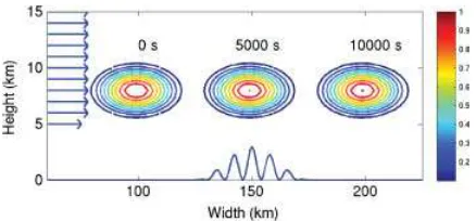
Figure 1.Results from the Cut-cell model for the advection test. Contours indicate the tracer bubble concentration according to the colour bar with intervals of 0.1 and ranging from−0.2 to 1. The position of the bubble is indicated at three times 0, 5000 and 10 000 s after the introduction of the bubble on the left. The domain shown is 150 km wide and 15 km high centred on the orography which is indicated by the blue line at the base. The vectors down the left show the wind profile, large vectors have a magnitude of 10 m s−1.
pressure gradient calculation. The errors can be vanish-ingly small for nearly linear vertical pressure gradients. By introducing an inversion layer, the nearby verti-cal pressure gradients become very non-linear, causing small errors in the horizontal pressure gradient cal-culation which induce spurious motion. To highlight these errors, an inversion is included in this test. The background potential temperature profile is a constant 300 K. The potential temperature perturbations are non-zero such that the full potential temperature pro-file varies with the Brunt–V¨ais¨ala frequency (N) and has an inversion between 2 and 3 km. Below 2 km and above 3 kmN=0.1 s−1 whereas between 2 and 3 km
N=0.2 s−1. The initial wind field is set to zero and the simulation is run out to 5 h with a time-step of 1.01 s. After 5 h the maximum vertical velocity in the cut-cell experiment is 10−12m s−1≈0 m s−1 to machine accuracy and the horizontal velocities are identically zero. By comparison, for terrain-following models Klemp (2011) reports a maximum velocity of 1 m s−1 for the basic terrain-following methods (BTF/HTF) and 0.1 m s−1 for the more sophisticated methods (STF/SLEVE).
Increasing the height of the hill up to at least 4000 m does not change this result for the Cut-cell model. This confirms that a correctly implemented cut-cell model does not suffer the spuriously generated winds associated with terrain-following models.
3.2. Advection test
Sch¨aret al.(2002) demonstrated errors due to terrain-following coordinates with a simple advection test. This test is reproduced here with the cut-cell model.
A bubble of tracer is blown across a mountain range with a wind profile that is zero below the mountain tops and constant above 5 km is described by
u(z)=
u0 z2≤z
u0sin2
π 2
z−z1 z2−z1
z1≤z ≤z2
0 z ≤z1
where u0=10 m s−1, z1=4 km and z2=5 km, see Figure 1. The initial tracer concentration is described by
q(x,z)=
cos2πr 2
r ≤1
0 otherwise (2)
where
r =
x−x0
Ax 2
+
z −z0
Az
212
and Az=3 km is the vertical radius, Ax=25 km is the horizontal radius and the bubble is centred at
x0=100 km, z0=9 km. The domain is 300 km wide and 25 km high with a horizontal grid spacing of 1000 m and a vertical grid spacing of 500 m. In the centre of the bottom boundary is a sinusoidal mountain range described by Equation 1 from the resting atmosphere test withh0=3 km,a=25 km and
γ=8 km. The atmosphere is neutrally stratified with a constant potential temperature of 300 K and the model is run for 10 000 s so that the bubble passes once across the mountain range.
The results from the cut-cell model are shown in Figure 1. Results have been compared (though not shown) to the same run with no orography. The differences between the two simulated bubbles were exactly zero confirming that any observed differences along the trajectory are due to the advection scheme and not the representation of terrain. Furthermore, moving the bubble closer to the top of the mountains does not change the results suggesting there is no undue influence from the terrain on the flow aloft.
Sch¨ar et al. (2002, Figure 6) demonstrate that the basic terrain-following coordinates induce distur-bances which visibly distort the bubble downstream of the mountain range. By removing the terrain influ-ence more rapidly with height, the SLEVE coordinate exhibits much improved results (Schaer et al. (2002) Figure 6c,d), similar to those described here. Regayre
et al. (2013) shows that bringing the tracer bubble closer to the hill affects the evolution of the bub-ble downstream of the mountain range when terrain-following methods are used.
3.3. Rising bubble
Idealized simulations of the cut-cell method of representing orography 47
flows over small hills. The model solves the time-dependent Boussinesq equations in a BTF (Gal-Chen and Somerville, 1975) terrain-following coordinate system and utilises a finite-difference discretisation and an explicit time integration scheme. For these simulations a centred-difference advection scheme was used and the turbulence closure scheme was turned off to keep the numerics as similar to the Cut-cell model as possible.
The Cut-cell model and BLASIUS were both set up with a no-slip condition imposed at the lower boundary, periodic lateral boundary conditions and a rigid-lid upper boundary condition. A round, warm potential temperature perturbation with a Gaussian profile is initialized in the centre of a domain 20 km wide and 20 km high, with a uniform grid spacing of 100 m. The bubble is described by
θ′(x,z)=
cos2π2r r ≤1
0 otherwise (3)
where
r =
x −x0
Ax 2
+
z −z0
Az
212
and Az=2 km is the vertical radius, Ax=2 km is the horizontal radius and the bubble is centred at
x0=10 km, z0=4.5 km.
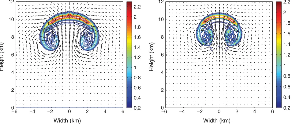
The atmosphere is neutrally stable with a back-ground potential temperature of 300 K and the model is run out to 1000 s. Several runs are completed with the cut-cell model with different terrain at the lower boundary and repeated with the terrain-following model BLASIUS. Figure 2 shows the evolution of the bubble in the no-hill case with a flat lower boundary for both the Cut-cell model and BLASIUS. These are
similar to the bubble produced by Bryan and Fritsch (2002) and are used as a reference in the discussion below.
Three different runs are made each with a bell-shaped hill described by
h(x)= h0 1+x2
a2
(4)
with a maximum height (h0) of 1,000 m and three different half widths (a) of 3,000 m, 2,000 m and 1,000 m. The key difference between these hills is the gradient of their slopes which increases as the width decreases indicated by the aspect ratio (h0/a) increasing from 1/3 to 1/2 to 1. As indicated by the wind vectors in Figure 2, the winds are not strong below 1,100 m: for both models, the maximum wind speed below 1,100 m remains more than an order of magnitude smaller than the maximum further aloft, at all times throughout the simulation, and for all hills. Therefore, as the hill is far beneath the bubble, where the winds are not strong, the different hills should not significantly impact the evolution of the bubble.
The Cut-cell model uses a time-step of 10−3 s due to the restrictions on the CFL condition because of the small cut-cells at the boundary. BLASIUS uses a variable time-step dependent on the CFL condition of about 1.3 s. Tests have been run with BLASIUS for smaller fixed time-steps of 0.1 s and 0.01 s for the steepest hill (not shown) and no significant differences in the results were observed. Therefore we are confident that the results for the terrain-following model are not strongly dependent on the time-step.
For both models the result from each hill is sub-tracted from the respective no hill case and the dif-ferences are plotted in Figure 3. For the Cut-cell
−6 −4 −2 0 2 4 6
0 2 4 6 8 10 12
Width (km)
Height (km)
0.2 0.4 0.6 0.8 1 1.2 1.4 1.6 1.8 2 2.2
Width (km)
Height (km)
−6 −4 −2 0 2 4 6
0 2 4 6 8 10 12
[image:5.595.62.539.535.739.2]0.2 0.4 0.6 0.8 1 1.2 1.4 1.6 1.8 2 2.2
Figure 2.Potential temperature perturbations for the warm bubble after 1000 s from the Cut-cell model (a) and BLASIUS (b). The contour interval is 0.1 K. The vectors indicate the wind velocity. The maximum vertical velocity in (a) is 15.61 m s−1and in (b) is 17.17 m s−1
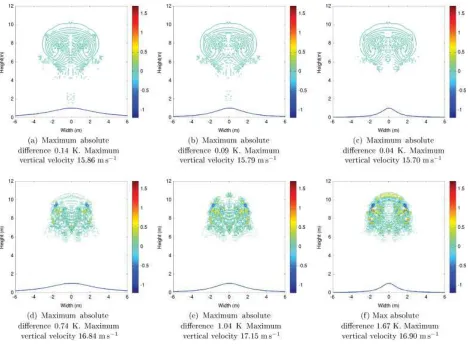
Figure 3.Potential temperature difference plots at time t=1000 s. Differences are between the warm rising bubble with no hill and 1000 m high hills of different half-widths. For (a) and (d)a=3 km, for (b) and (e)a=2 km and for (c) and (f)a=1 km wide. Panels (a–c) are from the cut-cell model and panels (d–f) are from the terrain-following model, BLASIUS. Differences are in K the contour interval is 0.1 K ranging from−1.2 to 1.7 K. The maximum absolute potential difference is given beneath each subfigure, along with the maximum vertical velocity.
model the difference is a straightforward subtraction. However as the computational grid is different for each hill with BLASIUS the results are first interpolated lin-early onto a regular grid before subtracting. The errors of this interpolation are of the order 10−3 K, 3 orders of magnitude smaller than the differences plotted in Figure 3 and therefore do not significantly contribute to the results.
The differences with the cut-cell model are an order of magnitude smaller than the differences with the terrain-following model and do not increase as
h0/a increases from 1/3 to 1. The differences in the BLASIUS plots on the other hand increase as the aspect ratio increases, from a max of 0.70 K when the ratio is 1/3 to a max of 1.67 K when it is 1. The increase in differences from BLASIUS as h0/a
increases indicates a worsening in the solution as the computational grid becomes increasingly deformed and for steeper hills, with aspect ratios greater than 1, BLASIUS no longer converges to a solution. This problem is not encountered with the Cut-cell model, whose computational grid away from the lower boundary is not affected by the presence of orography. The Cut-cell model has been successfully run with hills having aspect ratios up to 10. Though not shown,
the results remain consistent with those presented here, showing little change in the magnitude of the differences from the no-hill case.
4. Conclusions
Idealized simulations of the cut-cell method of representing orography 49
computational grid away from the terrain, the cut-cell method reduces errors in the flow aloft compared to terrain-following methods. Furthermore, results from the rising bubble test with very steep orography (aspect ratio of 10) demonstrate that the Cut-cell model is stable, without compromising accuracy. This is impor-tant for large scale models and in representing features such as wave propagation.
Acknowledgements
The authors would like to acknowledge the support of a NERC studentship and use of JASMIN/NERC computer facilities. Gadian, Lock and Ross were partially funded in this work by Natural Environment Research Council grants NE/I022094/1 and NE/K006746/1.
References
Adcroft A, Hill C, Marshall J. 1997. Representation of topography by shaved cells in a height coordinate ocean model.Monthly Weather
Review125: 2293–2315.
Bonaventura L. 2000. A semi-implicit semi-lagrangian scheme using the height coordinate for a nonhydrostatic and fully elastic model of atmospheric flows.Journal of Computational Physics158: 186–213.
Botta N, Klein R, Langenberg S, Luetzenkirchen S. 2004. Well balanced finite volume methods for nearly hydrostatic flows.Journal
of Computational Physics196: 539–565.
Bryan G, Fritsch JM. 2002. A benchmark simulation for moist nonhydrostatic numerical models. Monthly Weather Review 130: 2917–2928.
Gal-Chen T, Somerville RCJ. 1975. On the use of a coordinate transformation for the solution of the Navier– Stokes equations.
Journal of Computational Physics17: 209–228.
Gallus WA, Klemp J. 2000. Behavior of flow over step orography.
Monthly Weather Review128: 1153–1164.
Janjic ZI. 1989. On the pressure gradient force error inσ-coordinate spectral models.Monthly Weather Review117: 2285–2292. Jebens S, Knoth O, Weiner R. 2011. Partially implicit peer methods for
the compressible Euler equations.Journal of Computational Physics 230: 4955–4974.
Klein R, Bates KR, Nikiforakis N. 2009. Well-balanced compressible cut-cell simulation of atmospheric flow.Philosophical Transaction
of Royal Society London A367: 4559–4575.
Klemp J. 2011. A terrain-following coordinate with smoothed coordi-nate surfaces.Monthly Weather Review139: 2163–2169.
Klemp JB, Wilhelmson RB. 1978. The simulation of three-dimensional convective storm dynamics.Journal of the Atmospheric Sciences35: 1070–1096.
Lock S-J. Development of a new numerical model for studying microscale atmospheric dynamics. PhD thesis, School of Earth and Environment, University of Leeds, 2008.
Lock S-J, Bitzer H, Coals A, Gadian A, Mobbs S. 2012. Demon-stration of a cut-cell representation of 3D orography for studies of
atmospheric flows over very steep hills. Monthly Weather Review 140: 411–424.
Leuenberger D, Koller M, Fuhrer O, Sch¨ar C. 2010. A generalization of the SLEVE vertical coordinate. Monthly Weather Review 138: 3683–3689.
McFarlane NA. 1987. The Effect of orographically excited gravity wave drag and the general circulation of the lower stratosphere and troposphere.Journal of the Atmospheric Sciences44: 1775–1800. McIlveen R. 1992.Fundamentals of Weather and Climate. Chapman
and Hall: London, UK.
Mesinger F, Janjic ZI, Nickovic S, Gavrilov D, Deaven DG. 1988. The step-mountain coordinate: model description and performance for cases of alpine lee cyclogenesis and for a case of an Appalachian redevelopment.Monthly Weather Review116: 1493–1518. Regayre, LA, Ross AN, Lock S-J. 2013: A new terrain-following
coordinate transformation with improved accuracy. Quart. J. Roy.
Meteor. Soc., (submitted).
Sch¨ar C, Leuenberger D, Fuhrer O, Luthi D, Girad C. 2002. A new terrain following vertical coordinate formulation for atmospheric prediction models.Monthly Weather Review138: 2459–2480. Simmons AJ, Burridge DM. 1981. An energy and angular momentum
conserving vertical finite difference scheme and hybrid vertical coordinates.Monthly Weather Review109: 758–766.
Steppeler J, Bitzer H, Minotte M, Bonaventura L. 2002. Nonhydrostatic atmospheric modeling using a Z-coordinate representation.Monthly
Weather Review 130: 2143–2149.
Steppeler J, Bitzer HW, Janjic Z, Sch¨attler U, Prohl P, Gjertsen U, Torrisi L, Parfinievicz J, Avgoustoglou E, Damrath U. 2006. Prediction of clouds and rain using a z-coordinate non-hydrostatic model.Monthly Weather Review134: 3625–3643.
Steppeler J, Park SH, Dobler A. 2011. A 5-day hindcast experiment using a cut cell z-coordinate model.Atmospheric Science Letters12: 340–344.
Steppeler J, Park S-H, Dobler A. 2013. Forecasts covering one month using a cut cell model.Geoscientific Model Development6: 875–882.
N. Wood. Turbulent flow over three-dimensional hills. PhD thesis, University of Reading, 1992.
Wood N, Mason PJ. 1993. The pressure force induced by neutral, turbulent flow over hills.Quarterly Journal of Royal Meteorological
Society119: 1233–1267.
Yamazaki H, Satomura T. 2008. Vertically combined shaved cell model in a z-coordinate nonhydrostatic atmospheric model. Atmospheric
Science Letters9: 171–175.
Yamazaki H, Satomura T. 2010. Nonhydrostatic atmospheric modeling using a combined cartesian grid. Monthly Weather Review 138: 3932–3945.
Yamazaki H, Satomura T. 2012. Non-hydrostatic atmospheric cut cell model on a block-structured mesh.Atmospheric Science Letters13: 29–35.
Z¨angl G. 2002. An improved method for computing horizontal dif-fusion in a sigma-coordinate model and its application to simula-tions over mountainous topography.Monthly Weather Review 130: 1423–1432.
Z¨angl G. 2012. Extending the numerical stability limit of terrain-following coordinate models over steep slopes. Monthly Weather
Review140: 3722–3733.