This is a repository copy of
A progressive refinement approach for the visualisation of
implicit surfaces
.
White Rose Research Online URL for this paper:
http://eprints.whiterose.ac.uk/3761/
Book Section:
Gamito, M.N. and Maddock, S.C. (2007) A progressive refinement approach for the
visualisation of implicit surfaces. In: Braz, J., Ranchordas, A., Araújo, H. and Jorge, J.,
(eds.) Advances in Computer Graphics and Computer Vision : International Conferences
VISAPP and GRAPP 2006, Setúbal, Portugal, February 25-28, 2006, Revised Selected
Papers. Communications in Computer and Information Science, 4 (Part 3). Springer ,
Berlin Heidelberg , pp. 93-108. ISBN 978-3-540-75274-5
https://doi.org/10.1007/978-3-540-75274-5_6
[email protected] https://eprints.whiterose.ac.uk/
Reuse
Unless indicated otherwise, fulltext items are protected by copyright with all rights reserved. The copyright exception in section 29 of the Copyright, Designs and Patents Act 1988 allows the making of a single copy solely for the purpose of non-commercial research or private study within the limits of fair dealing. The publisher or other rights-holder may allow further reproduction and re-use of this version - refer to the White Rose Research Online record for this item. Where records identify the publisher as the copyright holder, users can verify any specific terms of use on the publisher’s website.
Takedown
If you consider content in White Rose Research Online to be in breach of UK law, please notify us by
A PROGRESSIVE REFINEMENT APPROACH
FOR THE VISUALISATION OF IMPLICIT SURFACES
Manuel N. Gamito
∗, Steve C. Maddock
Department of Computer Science, The University of Sheffield [email protected], [email protected]
Keywords: Affine arithmetic, implicit surface, progressive refinement, ray casting.
Abstract: Visualising implicit surfaces with the ray casting method is a slow procedure. The design cycle of a new implicit surface is, therefore, fraught with long latency times as a user must wait for the surface to be rendered before being able to decide what changes should be introduced in the next iteration. In this paper, we present an attempt at reducing the design cycle of an implicit surface modeler by introducing a progressive refinement rendering approach to the visualisation of implicit surfaces. This progressive refinement renderer provides a quick previewing facility. It first displays a low quality estimate of what the final rendering is going to be and, as the computation progresses, increases the quality of this estimate at a steady rate. The progressive refinement algorithm is based on the adaptive subdivision of the viewing frustrum into smaller cells. An estimate for the variation of the implicit function inside each cell is obtained with an affine arithmetic range estimation technique. Overall, we show that our progressive refinement approach not only provides the user with visual feedback as the rendering advances but is also capable of completing the image faster than a conventional implicit surface rendering algorithm based on ray casting.
1
INTRODUCTION
Implicit surfaces play an important role in Computer Graphics. Surfaces exhibiting complex topologies, i.e. with many holes or disconnected pieces, can be easily modelled in implicit form. An implicit surface is defined as the set of all pointsxthat verify the
con-ditionf(x) = 0 for some functionf : R3 7→ R.
Modelling with implicit surfaces amounts to the con-struction of an appropriate functionf that will gener-ate the desired surface.
Rendering algorithms for implicit surfaces can be broadly divided into meshing algorithms and ray cast-ing algorithms. Meshcast-ing algorithms convert an im-plicit surface to a polygonal mesh format, which can be subsequently rendered in real time with modern graphics processor boards (Lorensen and Cline, 1987; Bloomenthal, 1988; Velho, 1996). Ray casting al-gorithms compute the projection of an implicit sur-face on the screen by casting rays from each pixel into three-dimensional space and finding their intersection with the surface (Roth, 1982).
∗Supported by grant SFRH/BD/16249/2004 from Fundac¸˜ao para a Ciˆencia e a Tecnologia, Portugal.
Our ultimate goal is to use implicit surfaces as a tool to model and visualise realistic procedural plan-ets over a very wide range of scales. The function
f that generates the surface terrain for such a planet must have fractal scaling properties and exhibit a large amount of small scale detail. Examples of this type of terrain generating function can be found in the Com-puter Graphics literature (Ebert et al., 2003). In our planet modelling scenario, meshing algorithms are too cumbersome as they generate meshes with a very high polygon count in order to preserve all the visible surface detail. Furthermore, as the viewing distance changes, the amount of surface detail varies accord-ingly and the whole polygon mesh needs to be regen-erated. For these reasons, we have preferred a ray casting approach because of its ability to render the surface directly without the need for an intermediate polygonal representation.
compounded by the fact that an anti-aliased image re-quires that many rays be shot for each pixel (Cook, 1989).
We propose to alleviate the long rendering times as-sociated with the modelling and subsequent ray cast-ing of complex fractal surfaces by providcast-ing a quick previewer based on a progressive refinement render-ing principle. The idea of progressive refinement for image rendering was first formalised in 1986 (Berg-man et al., 1986). Progressive refinement rendering has received much attention in the fields of radios-ity and global illumination (Cohen et al., 1988; Guo, 1998; Farrugia and Peroche, 2004). Progressive re-finement approaches to volume rendering have also been developed (Laur and Hanrahan, 1991; Lippert and Gross, 1995). Our previewer uses progressive rendering to visualise an increasingly better approx-imation to the final implicit surface. It allows the user to make quick editing decisions without having to wait for a full ray casting solution to be computed. Because the rendering is progressive, the previewer can be terminated as soon as the user is satisfied or not with the look of the surface.
Our progressive refinement previewing method re-lies on affine arithmetic to compute an estimate of the variation of the implicit functionf inside some re-gion (Comba and Stolfi, 1993). Affine arithmetic is a framework for evaluating algebraic functions with arguments that are bounded but otherwise unknown. It is a generalisation of the older interval arithmetic framework (Moore, 1966). Affine arithmetic, when compared against interval arithmetic, is capable of returning much tighter estimates for the variation of a function, given input arguments that vary over the same given range. Affine arithmetic has been used with success in an increasing number of Computer Graphics problems, including the ray casting of im-plicit surfaces (de Cusatis Jr. et al., 1999). We use a simpler form of affine arithmetic known as Affine Form 1 (AF1), which we term reduced affine arith-metic (Messine, 2002). Reduced affine aritharith-metic, in the context of ray casting implicit surfaces made from procedural fractal functions, returns the same results as standard affine arithmetic while being faster to compute and requiring smaller data structures.
2
PREVIOUS WORK
One of the best known techniques for previewing implicit surfaces at interactive frame rates is based on the dynamic placement of discs that are tangent to the surface (Witkin and Heckbert, 1994; Hart et al., 2002). The discs are kept apart by the application of repulsive forces and are constrained to remain on the implicit surface. Each disc is also made tangent to
the surface by sharing the surface normal at the point where it is located. This previewing system relies on a characteristic of our visual system whereby we are able to infer the existence of an object based solely on the distribution of a small number of features on the surface of that object. This visual trait only works, however, when the surface of the object is simple and fairly smooth. If the surface is irregular, an apparently random distribution of discs is visible and no object is perceived.
An approximate representation of an implicit sur-face can be generated by subdividing the space in which the surface is embedded into progressively smaller voxels and using a surface classification tech-nique to identify which voxels are potentially inter-secting with the surface. One such spatial subdivi-sion method employs interval arithmetic to perform the surface classification step (Duff, 1992). The sub-division strategy of this method is adapted from an earlier work and is not suitable for interactive pre-viewing (Woodwark and Quinlan, 1982). One must wait for the subdivision to finish before any surface approximation can be visualised unless some addi-tional data processing is added, which will tend to slow down the algorithm. Another spatial subdivision method employs affine arithmetic to perform surface classification and subdivides space with an octree data structure (de Figueiredo and Stolfi, 1996). The octree voxels are rendered from back to front, relative to the viewpoint, with a painter’s algorithm. This subdivi-sion strategy is wasteful as it tracks the entire surface through subdivision, including parts that are occluded and that could be safely discarded for a given viewing configuration.
3
RENDERING WITH
PROGRESSIVE REFINEMENT
The main stage of our method consists in the binary subdivision of the space, visible from the camera, into progressively smaller cells that are known to straddle the boundary of the surface. The subdivision mechan-ism stops as soon as the projected size of a cell on the screen becomes smaller than the size of a pixel. In-formation about the behaviour of the implicit function
f inside a cell is returned by evaluating the function with reduced affine arithmetic. The procedure for ren-dering implicit surfaces with progressive refinement can be broken down into the following steps:
1. Build an initial cell coincident with the camera’s viewing frustrum. The near and far clipping planes are determined so as to bound the implicit surface.
2. Recursively subdivide this cell into smaller cells. Discard cells that do not intersect with the implicit surface. Stop subdivision if the size of the cell’s projection on the image plane falls below the size of a pixel.
3. Assign the shading value of a cell to all pixels that are contained inside its projection on the image plane. The shading value for a cell is taken from the evaluation of the shading model at the centre point of the cell.
The following sections will explain how each of the steps in our rendering method work, starting with a presentation of the reduced affine arithmetic frame-work in Section 3.1. We then explain the geometry of a cell inside the camera’s viewing frustrum (Sec-tion 3.2) and how a cell is subdivided and rendered (Sections 3.3 and 3.4). We also explain in Section 3.5 how a region of interest can be optionally defined so as to provide the user with interactive control during the rendering process.
3.1
Reduced Affine Arithmetic
A variable is represented with reduced affine arith-metic (rAA) as a central value plus a series of noise symbols. In contrast to the standard affine arith-metic model, the number of noise symbols is con-stant and can be used to describe the fundamental degrees of freedom of the problem under considera-tion (Messine, 2002). In the rendering method that is being described in this paper, the degrees of freedom are the three parameters necessary to locate any point inside the viewing frustrum of the camera. These parameters are the horizontal distanceualong the im-age plane, the vertical distancevalong the same im-age plane and the distancetalong the ray that passes through the point at(u, v). A rAA variableˆa has,
therefore, the following representation:
ˆ
a=a0+aueu+avev+atet+akek. (1)
The noise symbolseu,evandetare shared between
all rAA variables in the system, which allows for the representation of correlation information between rAA variables relative to the u, v andt degrees of freedom. The extra noise symbolekis included to
ac-count for uncertainties in theaˆvariable that are not shared with any other variable.
Operations on rAA variables are performed by up-dating theau,avandatnoise coefficients with their
new uncertainties and clumping all other uncertain-ties into the ak coefficient. We give an example of
how rAA operations work by considering the case of the multiplication between two variablesˆaandˆb of the form (1). In the original standard affine arithmetic framework, the resultˆc= ˆaˆbwould be written as:
ˆ
c=c0+cueu+cvev+ctet+
+ckaeka+ckbekb+cnen. (2)
The final error symbols fromˆaandˆbwere written as
ekaandekb, respectively, to make it clear that they are
independent. The new noise symbolen is introduced
to account for the non-linearity of the multiplication operator. The coefficients for the variableˆcare:
c0=a0b0,
cu=a0bu+b0au,
cv=a0bv+b0av,
ct=a0bt+b0at,
cka=b0ak,
ckb=a0bk,
cn= (|au|+|av|+|at|+|ak|)× (|bu|+|bv|+|bt|+|bk|).
(3)
is condensed into a new variabledˆwith only four er-ror symbols, we will have for the coefficients ofdˆ:
d0=c0,
du=cu,
dv=cv,
dt=ct,
dk=|cka|+|ckb|+|cn|.
(4)
The condensed variabledˆis now in the rAA form, according to (1). With the reduced affine arithmetic framework, all operations are always followed by a condensation step to keep a constant number of er-ror symbols for every variable throughout the com-putation. In practice, all operations in reduced affine arithmetic are modified so that the condensation step (4) is automatically built into them. The multiplic-ationˆc = ˆaˆb, that in standard affine arithmetic was given by (3), now becomes:
c0=a0b0,
cu=a0bu+b0au,
cv=a0bv+b0av,
ct=a0bt+b0at,
ck=|a0bk|+|b0ak|+
(|au|+|av|+|at|+|ak|)× (|bu|+|bv|+|bt|+|bk|).
(5)
Reduced affine arithmetic is more efficient than standard affine arithmetic because it keeps only the required minimum amount of correlation information between all rAA quantities. In our progressive refine-ment renderer, much faster convergence rates can be obtained towards the final image by using affine arith-metic in reduced form.
For an implicit surface, the value f(x) at some
pointxin space can be computed with reduced
af-fine arithmetic. The rAA representationxˆof the
vec-torx is a tuple of three rAA coordinates, similar to
(1), where each coordinate has its own independent noise symboleki, withi = 1,2,3. The rAA vector
ˆ
xdescribes not a point but a region of space spanned
by the uncertainties associated with its three coordin-ates. Evaluation of the expressionyˆ=f(ˆx)leads to
a range estimateyˆfor the variation off(ˆx)inside the
region spanned byxˆ. Knowingyˆ, the average value ¯
yand the variancehyifor that range estimate can be computed as follows:
¯
y,y0, (6a)
hyi,|yu|+|yv|+|yt|+|yk|. (6b)
The range estimate yˆis then known to lie inside the interval[ ¯y− hyi, ¯y+hyi]. If this interval con-tains zero, the region spanned byxˆ may or may not
intersect with the implicit function. This is because
affine arithmetic (both in its standard and reduced forms) always computes conservative range estimates and it is possible that the exact range resulting from
f(ˆx)may be smaller thanyˆ. What is certain is that
if [ ¯y − hyi, ¯y+hyi] does not contain zero the re-gion spanned byxˆis either completely inside or
com-pletely outside the implicit surface and therefore does not intersect it.
3.2
The Anatomy of a Cell
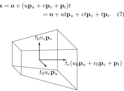
A cell is a portion of the camera’s viewing frustrum that results from a recursive subdivision along theu,
v andt parameters. Figure 1 depicts the geometry of a cell. It has the shape of a truncated pyramid of quadrangular cross-section, similar to the shape of the viewing frustrum itself. Four vectors, taken from the camera’s viewing system, are used to define the spa-tial extent of a cell. These vectors are:
The vectoro This is the location of the camera in the
world coordinate system.
The vectorspuandpv They represent the
hori-zontal and vertical direction along the image plane. The length of these vectors gives the width and height, respectively, of a pixel in the image plane.
The vectorpt It is the vector from the camera’s
viewpoint and orthogonal to the image plane. The length of this vector gives the distance from the viewpoint to the image plane.
The vectorspu,pvandptdefine a left-handed
per-spective viewing system. The position of any pointx
inside the cell is given by the following inverse per-spective transformation:
x=o+ (upu+vpv+pt)t
=o+utpu+vtpv+tpt. (7)
t0uepu
t0vepv
[image:5.612.321.521.481.628.2]te(u0pu+v0pv+pt)
Figure 1: The geometry of a cell. The vectors show the three medial axes of the cell.
The spatial extent of a cell is obtained from the above by having theu,v andtparameters vary over appropriate intervals [ua, ub], [va, vb]and [ta, tb].
variables must first be performed. The rAA variable
ˆ
u=u0+ueeuwill span the same interval[ua, ub]
asudoes if we have:
u0= (ub+ua)/2, (8a)
ue= (ub−ua)/2. (8b)
Similar results apply for the v and t parameters. Substitutinguˆ,vˆandtˆin (7) foru,vandt, we get:
x=o+t0u0pu+t0v0pv+t0pt +t0ueeupu+t0veevpv
+u0teetpu+v0teetpv+teetpt +teueeuetpu+teveevetpv.
(9)
The first line of (9) contains only constant terms. The second and third lines contain linear terms of the noise symbolseu,evandet. The fourth line contains
two non-linear termseuetandevet, which are a
con-sequence of the non-linearity of the perspective trans-formation. Since a rAA representation cannot accom-modate such non-linear terms they are replaced by the independent noise termsek1,ek2 andek3 for each of
the three cartesian coordinates ofxˆ. The rAA vector ˆ
xis finally given by:
ˆ
x=o+t0(u0pu+v0pv+pt) +t0uepueu+t0vepvev +te(u0pu+v0pv+pt)et + [xk1ek1 xk2ek2 xk3ek3]
T
,
(10)
with
xki =|teuepui|+|tevepvi|, i= 1,2,3. (11)
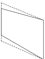
A consequence of the non-linearity of the perspect-ive projection and its subsequent approximation with rAA is that the region spanned byxˆis going to be
lar-ger than the spatial extent of the cell. Figure 2 shows the geometry of a cell and the region spanned by its rAA representation in profile. Because the rAA rep-resentation has been linearised, its spatial extent is a prism rather than a truncated pyramid. This has fur-ther consequences in that the evaluation off(ˆx) is
going to include information from the regions of the prism outside the cell and will, therefore, lead to range estimates that are larger than necessary. The linearisa-tion error is more pronounced for cells that exist early in the subdivision process. As subdivision continues and the cells become progressively smaller, their geo-metry becomes more like that of a prism and the dis-crepancy with the geometry ofxˆdecreases2.
The subdivision of a cell proceeds by first choos-ing one of the three perspective projection parameters
2
This can be demonstrated by the fact that the termsteue
andtevein (9) decrease more rapidly than any of the linear
termsue,ve andteof the same equation as the latter
[image:6.612.371.460.90.205.2]con-verge to zero.
Figure 2: The outline of a cell (solid line) and the outline of its rAA representation (dashed line) shown in profile. The rAA representation is a prism that forms a tight enclosure of the cell.
u,vortand splitting the cell in half along that para-meter. This scheme leads to a k-d tree of cells where the sequence of dimensional splits is only determined at run time. The choice of which parameter to split along is based on the average width, height and depth of the cell:
¯
wu= 2t0uekpuk, (12a) ¯
wv = 2t0vekpvk, (12b) ¯
wt= 2teku0pu+v0pv+ptk. (12c)
If, say, w¯u is the largest of these three measures,
the cell is split along theuparameter. The two child cells will have theiruparameters ranging inside the intervals [ua, u0]and[u0, ub], where[ua, ub]was
the interval spanned byuin the mother cell. In prac-tice, the factors of2 in (12) can be ignored without changing the outcome of the subdivision. This subdi-vision strategy ensures that, after a few iterations, all the cells will have an evenly distributed shape, even when the initial cell is very long and thin.
3.3
The Process of Cell Subdivision
ub−ua >1, (13a)
vb−va >1. (13b)
The values on the right hand sides of (13) are a con-sequence of the definition ofpuandpvin Section 3.2,
which cause all pixels to have a unit width and height. The sequence of events after a cell has been sub-divided depends on which of the parametersu,v or
twas used to perform the subdivision. If the subdi-vision occurred alongt, there will be two child cells with one in front of the other and totally occluding it. The front cell is first checked for the condition
0 ∈ f(ˆx). If the condition holds, the cell is pushed
into the priority queue and the back cell is ignored. If the condition does not hold, the back cell is also checked for the same condition. The difference now is that, if0 6∈f(ˆx)for the back cell, a new cell must
be searched by marching along thet direction. The first cell scanned, at the same subdivision level of the front and back cells, for which0 ∈ f(ˆx) holds is
the one that is pushed into the priority queue. On the other hand, if the subdivision occurred along theuor
vdirections, there will be two child cells that sit side by side relative to the camera without occluding each other. Both cells are processed in the same way. If, for any of the two cells,0 ∈ f(ˆx)holds, that cell is
[image:7.612.97.268.422.544.2]placed on the priority queue, otherwise a farther cell must be searched by marching forward in depth.
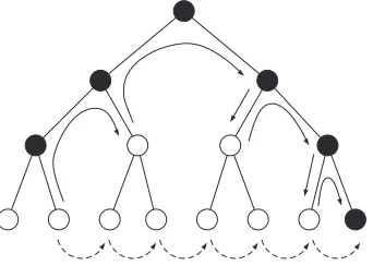
Figure 3: Scanning along the depth subdivision tree. Cells represented by black nodes may intersect with the surface. Cells represented by white nodes do not. The solid arrows show progression by depth-first order. The dotted arrows show progression by breadth-first order.
The process of marching forward from a cell along the depth directionttries to find a new cell that has a possibility of intersecting the implicit surface by verifying the condition0 ∈ f(ˆx). The process is
invoked when the starting cell has been determined not to verify the same condition. The reason for hav-ing this scannhav-ing in depth is because cells that do not intersect with the surface must be discarded. Only cells that verify0 ∈ f(ˆx)are allowed into the
pri-ority queue for further processing. Figure 3 shows
an example of this marching process. The scanning is performed by following a depth-first ordering re-lative to the tree that results from subdividing in t. The scanning sequence skips over the children of cells for which0 6∈ f(ˆx). The possibility of scanning in
breadth-first order, by marching along all the cells at the same level of subdivision, is not recommended be-cause in deeply subdivided trees a very high number of cells would have to be tested.
As mentioned before, when subdivision is per-formed alongt, the back cell is ignored whenever the front cell verifies0∈f(ˆx). This does not mean,
how-ever, that the volume occupied by this back cell will be totally discarded from further consideration. The front cell may happen to be subdivided during sub-sequent iterations of the algorithm and portions of the volume occupied by the back cell may then be revis-ited by the depth marching procedure.
3.4
Rendering a Cell
The shading value of a cell is obtained by evaluat-ing the shadevaluat-ing function at the centre of the cell. The central pointx0 for the cell is determined from (10)
to be:
x0=o+t0(u0pu+v0pv+pt). (14)
During rendering, the shading value of a cell is as-signed to all the pixels that are contained within its image plane projection. The centre of a pixel (i, j)
occupies the coordinates cij = (i+ 1/2, j+ 1/2)
on the image plane. All the pixels that verifycij ∈ [ua, ub]× [va, vb] for the cell being rendered will
be assigned its shading value. Any previous shad-ing values stored in these pixels will be overwritten. This process happens after cell subdivision and before the newly subdivided cells are placed on the priority queue. The subdivided cells will overwrite the shad-ing value of their mother cell on the image buffer. The same process also takes place for leaf cells before they are discarded. In this way, the image buffer always contains the best possible representation of the image at the start of every new iteration.
3.5
Specifying a Region of Interest
with the difference that the secondary queue is now being used. Once this queue becomes empty, the por-tion of the image inside the ROI is fully rendered and the algorithm returns to subdividing the cells that were left in the primary queue. It is also possible to cancel the ROI at any time by flushing any cells still in the secondary queue back to the primary queue.
3.6
Some Implementation Remarks
The best implementation strategy for our rendering method is to have an application that runs two threads concurrently: a subdivision thread and a rendering thread. An internal image buffer is used to store the rendering of the surface as it is being refined. The subdivision thread requires read-write access to this buffer while the rendering thread requires read-only access to the same buffer. The rendering thread is re-sponsible for periodically updating the graphical out-put of the application with the latest results from the subdivision thread. Its task is to invoke a single graph-ics library call that transfers the content of the internal image buffer to the frame buffer of the GPU card. A timer is used to keep a constant frame refresh rate. Except for the periodical invocation of the timer hand-ler routine, the rendering thread remains in a sleep state so that the subdivision thread can use all the CPU resources.
It is possible that, on machines with a small amount of main memory, excessive paging may occur due to the need to store a large number of samples in the pri-ority queue. We have implemented our application on a Pentium 4 1.8GHz with 1Gb of memory. All the results shown in the next section were tested on this computer and it was found that the use of swap memory was never necessary. In any case, it is advis-able that the data structure used to hold a sample be as light as possible.
4
RESULTS
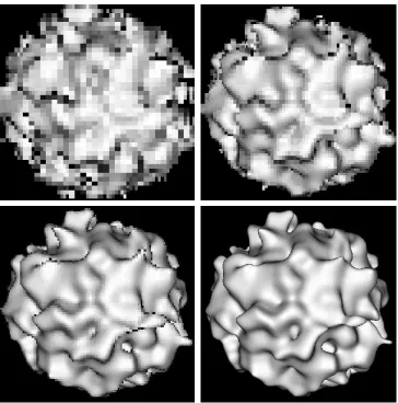
Figure 5 on the next page shows four snapshots taken during the progressive refinement rendering of an im-plicit sphere modulated with a Perlin procedural noise function (Perlin, 2002). The last snapshot shows the final rendering of the surface. The large scale features of the surface become settled quite early and the lat-ter stages of the refinement are mostly concerned with resolving small scale details.
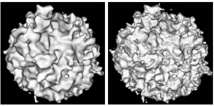
Figure 4 shows an implicit sphere modulated with two and three layers of the Perlin noise function. Table 1 shows the total number of iterations and the computation time for the surfaces that were rendered in Figures 4 and 5. The table also shows the computa-tion time for ray casting the same surfaces by
shoot-Figure 4: An implicit surface with two layers (left) and three layers (right) of a Perlin noise function.
[image:8.612.309.520.93.198.2]ing a single ray through the centre of each pixel. The number of iterations required to complete the pro-gressive rendering algorithm is largely independent of the complexity of each surface. It depends only on the image resolution and on the percentage of the image that is covered by the projected surface.
Table 1: Rendering statistics for an implicit sphere with sev-eral layers of Perlin noise.
Layers Iterations T ime Raycasting
1 350759 27.8s 1m10.4s
2 349465 1m16.8s 4m16.7s
3 359659 3m01.5s 8m51.7s
As estimated by the results in Table 1, preview-ing by progressive refinement is approximately three times faster than previewing by ray casting without anti-aliasing. It should be added that these numbers do not entirely reflect the reality of the situation be-cause, as demonstrated in the example of Figure 5, progressive refinement previewing already gives an accurate rendering of the surface at early stages of re-finement. From a perceptual point of view, therefore, the difference between the two previewing techniques is greater than what is shown in Table 1.
Figure 6 shows two snapshots of a progressive re-finement rendering where a region of interest is act-ive. The surface being rendered is the same two layer Perlin noise surface that was shown in Figure 4. The rectangular ROI is defined on the lower right corner of the image. The portion of the surface that projects inside the ROI is given priority during progressive re-finement.
[image:8.612.315.514.365.412.2]Figure 5: From left to right, top to bottom, snapshots taken during the progressive refinement rendering of a procedural noise function. The snapshots were taken after 5000, 10000, 28000 and 350759 iterations, respectively. The wall clock times at each snapshot are1.02s,1.98s,4.18s and27.80s, respectively.
[image:9.612.116.479.507.692.2]5
CONCLUSIONS
The rendering method, here presented, offers the pos-sibility of visualising implicit surfaces with progress-ive refinement. The main features of a surface be-come visible early in the rendering process, which makes this method ideal as a previewing tool dur-ing the editdur-ing stages of an implicit surface modeler. In comparison, a meshing method would generate expensive high resolution preview meshes for the more complex surfaces while a ray caster would be slower and without the progressive refinement fea-ture. Our rendering method, however, does not im-plement anti-aliasing and cannot compete with an anti-aliased ray caster as a production tool. Produc-tion quality renderings of some of the surfaces shown in this paper are typically done overnight, a fact which further justifies the need for a previewing tool.
It would have been straightforward to incorporate anti-aliasing into our rendering method by allowing cells to be subdivided down to sub-pixel size and then applying a low-pass filter to reconstruct the pixel samples. There is, however, one issue that prevents the use of our method for high quality renderings and which makes such implementation effort not worth-while. As explained in Section 3.1, the computation of range estimates with affine arithmetic is always conservative. This conservativeness implies that some cells a small distance away from the surface may be incorrectly flagged as intersecting with it. As a con-sequence, some portions of the surface may appear dilated after rendering. The offset error at some point on the surface is in the same order as the size of a pixel times the distance to the point. This artifact can be tolerated during previewing but is not acceptable for production quality renderings.
We intend in the future to apply our progressive re-finement previewing strategy not only to procedural fractal planets in implicit form but also to implicit sur-faces that interpolate scattered data points.
REFERENCES
Bergman, L., Fuchs, H., Grant, E., and Spach, S. (1986). Image rendering by adaptive refinement. In Evans, D. C. and Athay, R. J., editors, Computer Graphics (SIGGRAPH ’86 Proceedings), volume 20, pages 29– 37. ACM Press.
Bloomenthal, J. (1988). Polygonisation of implicit surfaces. Computer Aided Geometric Design, 5(4):341–355.
Cohen, M. F., Chen, S. E., Wallace, J. R., and Greenberg, D. P. (1988). A progressive refinement approach to fast radiosity image generation. In Dill, J., editor, Computer Graphics (SIGGRAPH ’88 Proceedings), volume 22, pages 75–84. ACM Press.
Comba, J. L. D. and Stolfi, J. (1993). Affine arithmetic and its applications to computer graphics. In Proc. VI Brazilian Symposium on Computer Graphics and Image Processing (SIBGRAPI ’93), pages 9–18. Cook, R. L. (1989). Stochastic sampling and distributed
ray tracing. In Glassner, A. S., editor, An Introduction to Ray Tracing, chapter 5, pages 161–199. Academic Press.
de Cusatis Jr., A., de Figueiredo, L. H., and Gattas, M. (1999). Interval methods for raycasting implicit sur-faces with affine arithmetic. In Proc. XII Brazilian Symposium on Computer Graphics and Image Pro-cessing (SIBGRAPI ’99), pages 65–71.
de Figueiredo, L. H. and Stolfi, J. (1996). Adaptive enu-meration of implicit surfaces with affine arithmetic. Computer Graphics Forum, 15(5):287–296.
Duff, T. (1992). Interval arithmetic and recursive subdivi-sion for implicit functions and constructive solid geo-metry. In Catmull, E. E., editor, Computer Graph-ics (SIGGRAPH ’92 Proceedings), volume 26, pages 131–138. ACM Press.
Ebert, D. S., Musgrave, F. K., Peachey, D. R., Perlin, K., and Worley, S. P. (2003). Texturing & Modeling: A Procedural Approach. Morgan Kaufmann Publishers Inc., 3rd edition.
Farrugia, J. P. and Peroche, B. (2004). A progressive ren-dering algorithm using an adaptive perceptually based image metric. Computer Graphics Forum, 23(3):605– 614.
Guo, B. (1998). Progressive radiance evaluation using dir-ectional coherence maps. In Beach, R. J., editor, Computer Graphics (SIGGRAPH ’98 Proceedings), volume 22, pages 255–266. ACM Press.
Hart, J. C., Jarosz, W., and Fleury, T. (2002). Using particles to sample and control more complex implicit surfaces. In Proceedings Shape Modeling International, pages 129–136.
Laur, D. and Hanrahan, P. (1991). Hierarchical splatting: A progressive refinement algorithm for volume ren-dering. In Sederberg, T. W., editor, Computer Graph-ics (SIGGRAPH ’91 Proceedings), volume 25, pages 285–288. ACM Press.
Lewis, J.-P. (1989). Algorithms for solid noise synthesis. In Lane, J., editor, Computer Graphics (SIGGRAPH ’89 Proceedings), volume 23, pages 263–270. ACM Press.
Lippert, L. and Gross, M. H. (1995). Fast wavelet based volume rendering by accumulation of transparent tex-ture maps. Computer Graphics Forum, 14(3):431– 444.
Lorensen, W. E. and Cline, H. E. (1987). Marching cubes: A high resolution 3D surface construction algorithm. In Stone, M. C., editor, Computer Graphics (SIG-GRAPH ’87 Proceedings), volume 21, pages 163– 169. ACM Press.
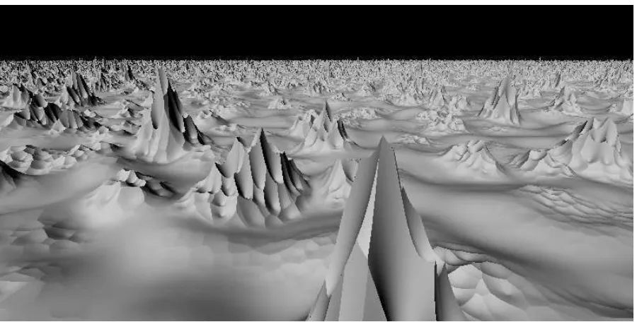
Figure 7: The visualisation of a procedural landscape that corresponds to a small section of an entire fractal planet. The image shows the final rendering result obtained with progressive refinement.
Rendering, pages 9–19, Bristol. Eurographics, Con-solidation Express Publishing.
Messine, F. (2002). Extentions to affine arithmetic: Applic-ation to unconstrained global optimizApplic-ation. Journal of Universal Computer Science, 8(11):992–1015.
Mitchell, D. P. (1990). Robust ray intersection with interval arithmetic. In Proceedings of Graphics Interface ’90, pages 68–74. Canadian Information Processing Soci-ety.
Moore, R. (1966). Interval Arithmetic. Prentice-Hall.
Painter, J. and Sloan, K. (1989). Antialiased ray tracing by adaptive progressive refinement. In Lane, J., ed-itor, Computer Graphics (SIGGRAPH ’89 Proceed-ings), volume 23, pages 281–288. ACM Press.
Perlin, K. (2002). Improving noise. ACM Transactions on Graphics (SIGGRAPH ’02 Proceedings), 21(3):681– 682.
Roth, S. D. (1982). Ray casting for modeling solids. Com-puter Graphics and Image Processing, 18(2):109– 144.
Stolfi, J. and de Figueiredo, L. H. (1997). Self-validated numerical methods and applications. Course notes for the 21st Brazilian Mathematics Colloquium.
Velho, L. (1996). Simple and efficient polygonization of implicit surfaces. Journal of Graphics Tools, 1(2):5– 24.
Whitted, T. (1980). An improved illumination model for shaded display. Communications of the ACM, 23(6):343–349.
Witkin, A. P. and Heckbert, P. S. (1994). Using particles to sample and control implicit surfaces. In Glassner, A.,
editor, Computer Graphics (SIGGRAPH ’94 Proceed-ings), volume 28, pages 269–278. ACM Press.
Woodwark, J. R. and Quinlan, K. M. (1982). Reducing the effect of complexity on volume model evaluation. Computer Aided Design, 14(2):89–95.