City, University of London Institutional Repository
Citation
: Salako, K. (2012). Extension to models of coincident failure in multiversion
software. (Unpublished Doctoral thesis, City University London)
This is the unspecified version of the paper.
This version of the publication may differ from the final published
version.
Permanent repository link:
http://openaccess.city.ac.uk/1302/
Link to published version
:
Copyright and reuse:
City Research Online aims to make research
outputs of City, University of London available to a wider audience.
Copyright and Moral Rights remain with the author(s) and/or copyright
holders. URLs from City Research Online may be freely distributed and
linked to.
City Research Online: http://openaccess.city.ac.uk/ [email protected]
M
ultiversion
S
oftware
by
Kizito Oluwaseun Salako
[email protected]
The Centre for Software Reliability
City University
London EC1V 0HB
United Kingdom
List of Figures 4
List of Symbols 6
Acknowledgments 9
Abstract 11
1 The Introduction 15
1.1 Reliability via Fault-Tolerance . . . 15
1.2 Layout of the Thesis . . . 19
2 Models Of Coincident Failure 21 2.1 Reference Scenario and Terminology . . . 23
2.2 Modelling System Failure . . . 24
2.3 Modelling the Development of a Program . . . 30
2.4 Modelling the Development of a 1–out–of–2 System . . . 37
2.5 EL and LM Model Results . . . 42
2.6 Visual Representations of the EL and LM models . . . 48
2.6.1 The EL/LM Model as a BBN . . . 49
2.6.2 Conditional Independence and BBN Transformations . . . 50
2.6.3 Difficulty Functions as Vectors . . . 53
2.7 Summary . . . 54
3 Generalised Models of Coincident Failure 57 3.1 Modelling Dependence between Version Developments . . . 58
3.2 Modelling Dependent Software Development Processes . . . 60
3.2.1 Justifying Conditional Independence in Practical Situations . . . 65
3.2.2 Effect of a single common influence . . . 68
3.2.3 The general case: multiple common influences . . . 69
3.2.4 Implications and interesting special cases . . . 70
3.3 Summary . . . 80
4 Geometric Models of Coincident Failure 83 4.1 Requirements for an Approach to ExtremisingPFDs . . . 84
4.2 A Geometric Approach to ExtremisingPFDs . . . 87
4.3 The Geometry of the LM Model . . . 88
4.4 Transformation between Bases . . . 95
4.5 A Brief Clarification On Notation . . . 101
4.6 Extremisation via Angles, Magnitudes and Planes . . . 102
4.7 Preliminary Results of Geometry–based Extremisation . . . 109
4.7.1 Angles with Demand Profile under Weak Constraints . . . 109
4.7.2 Relationship between Magnitudes, Angles and Projections . . . 110
4.7.3 Extremisation in Subspaces . . . 111
4.7.4 Largest Difficulty Function with Specified Mean . . . 117
4.8 Summary . . . 122
5 Bounds on Expected System PFD 125 5.1 Reasons for Bounding the Expected System PFD . . . 126
5.2 Forced Diversity vs Natural Diversity . . . 128
5.2.1 Preliminary Bounds when Forcing Diversity . . . 129
5.2.2 Forced Diversity under Indifference between Methodologies . . . 133
5.3 Optimisation of Expected System Pfd under Forced Diversity . . . 137
5.3.1 Extremisation ofqAB (given a Demand Profile) . . . 138
5.3.2 Extremisation ofqAB (given a Demand Profile,qB andqBB) . . . 138
5.3.3 Extremisation ofqAB (given a Demand Profile and Difficulty Function) 139 5.3.4 Extremisation ofqAB (given Demand Profile,qA, Difficulty Function) 141 5.3.5 Extremisation ofqAB (given values forqA, qB, qAA, andqBB) . . . 146
5.3.6 Maximisation ofqAB (given a Demand Profile,qA andqB) . . . 150
5.3.7 Maximisation ofqAB (given a Demand Profile,qAA andqBB) . . . 152
5.4 Summary . . . 152
6 Summary of Main Conclusions 161 6.1 Models of Controlled Team Interaction . . . 161
6.1.1 Decoupling Channel Development Processes . . . 162
6.1.2 The Independent Sampling Assumption . . . 165
6.1.3 Common Influences . . . 169
6.1.4 Modelling Results and Practical Considerations . . . 169
6.2 Geometric Model of Coincident Failure . . . 173
6.2.1 Benefits of Geometry-based Analyses . . . 174
6.2.2 Results and Practical Considerations . . . 178
7 Suggestions for Future Work 187 A Finite–Dimensional, Real Inner–Product Spaces 190 A.1 Vectors, Vector Spaces and Basis Vectors . . . 190
A.2 Real Inner–Product . . . 197
A.3 Orthogonality and Collinearity . . . 203
B Negative Correlation in Diversity Experiments 207 C The LM Model: Interpretations and Applications 214 C.1 A Characterization of Isolated Teams . . . 214
C.2 Conditionally Independent Version Sampling Distributions . . . 216
C.3 Relationships Between The EL and LM Models . . . 218
C.4 Modelling Non–linear Software Development Frameworks . . . 219
C.6 Cost Considerations . . . 220
C.7 Definitions of Terms and Concepts in The LM Model . . . 221
C.7.1 Relationship Between The Score Function and Correctness . . . 221
C.7.2 The Demand Space, Program Space and Score Function . . . 221
C.7.3 The (In)divisibility of Programs . . . 224
C.7.4 Subjective vs Objective Probabilities . . . 224
C.7.5 The Definition of Program and System Failure . . . 225
2.1 Plant Safety Protection System . . . 23
2.2 Demands and Internal Program–State . . . 28
2.3 Software Failure Regions . . . 29
2.4 BBN of Single–version development process . . . 32
2.5 BBN of LM model . . . 49
2.6 An Extension of the LM–Model BBN topology . . . 51
2.7 An Extension of the LM–Model BBN topology . . . 51
2.8 Difficulty functions as vectors . . . 54
3.1 BBN of LM model . . . 62
3.2 BBN of conditionally independent development, in the abstract . . . 62
3.3 Example BBN of typical development process . . . 63
3.4 Canonical form of BBN for conditionally independent development . . . 64
3.5 BBN with single common influence . . . 68
3.6 BBN ofdecoupled development processes . . . 73
4.1 Geometric Extremisation of PFDs . . . 87
4.2 Untransformed Basis Vectors . . . 96
4.3 Transformed Basis vectors . . . 97
4.4 “Worst” version in orthogonal basis . . . 97
4.5 “Worst” version in orthonormal basis . . . 98
4.6 Failure Regions as vectors . . . 100
4.7 Difficulty Functions as Vectors . . . 100
4.8 Expectedpfd as projections . . . 103
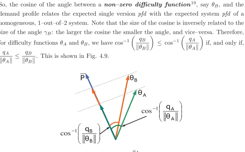
4.9 Cosine of angles with demand profile . . . 104
4.10 Variance vector . . . 105
4.11 Cosine and magnitude . . . 106
4.12 A plane inRn . . . 107
4.13 Planar representation of averages . . . 108
4.14 Parallel Planes . . . 109
4.15 Size of Difficulty Functions with Fixed Means . . . 111
4.16 Fixed Angles from demand profile . . . 112
4.17 Diagonals in subspaces . . . 116
4.18 qBB≤qB . . . 116
4.19 MaximumqBB in 2–dimensions . . . 118
5.1 Distribution of Expected System PFD . . . 129
5.2 Reliability Under Forced Diversity: Equal expected systempfds . . . 131
5.3 Reliability Under Forced Diversity: Orthogonal Difficulty Functions . . . 132
5.4 Reliability Under Forced Diversity: One Constant Difficulty Function . . . . 132
5.5 qAB Maximisation, givenθB . . . 142
5.6 Attainable Lower Bound: √qA qAA ≤ qB √ qBB and √ qBB≤ √qAA . . . 148
5.7 Attainable Upper Bound: √qqA AA ≤ qB √q BB and√qAA≤ √qBB. . . 149
5.8 qAB Maximisation givenqAAandqBB . . . 152
5.9 Demand profile that maximisesqAB . . . 157
5.10 Distribution ofθAwhich maximisesqAB . . . 158
5.11 Distribution ofθB which maximisesqAB . . . 159
5.12 Difficulty functions and demand profile that maximiseqAB . . . 160
6.1 Generalised Model of Coincident Failure with Conditional Independence . . . 163
6.2 Generalised Model of Coincident Failure with Some Decoupling . . . 166
6.3 LM Model . . . 167
6.4 “Completely” Decoupled Development Processes . . . 168
6.5 Space of scenarios and results . . . 170
6.6 Model of Coincident Failure: Decoupling Possible . . . 171
6.7 Results from Model of Coincident Failure: Decoupling Possible . . . 172
6.8 Diagonals in subspaces . . . 176
6.9 Geometric Model of Coincident Software Failure . . . 181
6.10 Constrained Optimisation ofqAB: Summary of Results . . . 182
6.11 Constrained Optimisation ofqAB: Summary of Results (contd.) . . . 183
6.12 Constrained Optimisation ofqAB: Summary of Results (contd.) . . . 184
6.13 Constrained Optimisation ofqAB: Summary of Results (contd.) . . . 185
6.14 Forced Diversityvs Natural Diversity . . . 186
A.1 Vectors as arrows . . . 194
A.2 Vector Addition . . . 194
A.3 Scalar Multiplication . . . 195
A.4 Standard Basis inRn. . . 196
A.5 Projections of unit vectors . . . 199
A.6 Projections of sums of vectors . . . 199
A.7 Angle between two vectors . . . 203
C.1 Summary of LM Model . . . 215
EL Eckhardt and Lee Model . . . 17
LM Littlewood and Miller Model . . . 17
ISA The Independent Sampling Assumption . . . 18
pfd Probability of failure on demand . . . 24
(X,ΣX,PX(·)) Probabilistic model of demand occurrence . . . 25
X Demand space . . . 25
ΣX Sigma–algebra of events in model of demand occurrence . . . 25
X Random variable defined over the demand space . . . 26
PX(·) Probability measure that defines the distribution ofX . . . 26
pmf Probability mass function . . . 26
ω(π, x) Score function, for versionπ, that is defined on demand space . . . 29
E Y(·) Mathematical expectation with respect to the distribution of Y . . . 30
Cov Y (·,·) Covariance of a pair of random variables that are both functions of the random variable Y . . . 30
di Theith software development process activity . . . 31
di A realisation of the random variable Di . . . 31
Ωdi Sample space for theith software development process activity . . . 31
Σdi Event space for theith software development process activity . . . .31
Di Random variable defined over the sample space, Ωdi . . . 31
PDi(·|d(i−1), . . . , d1) Probability measure that defines conditionalDidistribution . . . .31
Ωdi,Σdi,PDi(·|d(i−1), . . . , d1) Probabilistic model of development process activitydi . . . 31
P Set of all programs of interest . . . 33
ΣP Event space for single–version development process . . . 33
Π Random variable defined over the set of all programs,P . . . 33
(P,ΣP,PΠ(·|di, . . . , d1)) Conditional probabilistic model of final software deployment . . . 33
PΠ(·) Probability measure that defines distribution of Π . . . 33
PΠ(·|di, . . . , d1)
Probability measure that defines conditional distribution of Π . . . 33
Ωd1×. . .×Ωdn−1×P
Sample space for single–version development process model . . . .34
ΣΩd1,...,Ωdn−1,P Event space for single–version development process model . . . 34
P
D1,...,D(n−1),Π Probability measure that defines the joint distribution of{D1, . . . ,Π} . . . 34
θ(x) Difficulty function defined on demand space . . . 36
ΠA The random variable modelling the development of a version – either according to
methodology A or with respect to channel A . . . 38
θA(x)
Difficulty function – either induced by use of methodology A or related to channel A’s development . . . 42
θ1(x) Difficulty function related to channel 1’s development . . . 43
qAA The expected systempfd of a 1–out–of–2 system with channels built using the same
methodology . . . 47
qAB
The expected system pfd of a 1–out–of–2 system with one channel built using methodologyAand the other channel built using methodologyB . . . 47
θA;e1,...,eN(x)
The Difficulty function, related to channel A, that is defined over a set of N activities and the demand space . . . 70
θA;e1,...,eN θA;e1,...,eN(x) . . . 70
θA∗(xi) orθA∗i ith component of the vector denoted byθA(or θ∗A) in the basis
¯
P1, . . . ,P¯n
. . 89
¯
P1, . . . ,P¯n
The basis in which the components of vectors of interest are difficulty functions 91
ˆ
P1, . . . ,Pˆn
The basis of unit vectors in the direction of the vectorsP¯1, . . . ,P¯n
. . . 92
Pi Shorthand for the symbol PX(xi) . . . 95
¯
P Vector that models the difficulty function which fails on all demands . . . 99
θA or θ∗A The vector whoseith component in basis
¯
P1, . . . ,P¯n
isθA∗i . . . 101
θA(xi) orθAi ith component of the vector denoted byθA(or θ∗A) in the basis
ˆ
P1, . . . ,Pˆn
.101
V A vector space . . . 190
Rn The set ofn–tuples of real numbers . . . 191
V¯ Norm/length/size of the vector ¯V in an inner–product space . . . 197
ˆ
A Unit vector in the direction of the vector ¯Ain an inner–product space . . . 197
¯
I would like to thank and acknowledge my supervisor, Lorenzo Strigini, for his helpful guid-ance, deep insight, attention to detail and collaboration since my joining CSR (The Centre for Software Reliability).
In particular, I would like to acknowledge the following contributions he has made. An initial statement and proof of Eq. (2.19), on page 48. This equation shows, under a form of indifference between two development process methodologies, forcing diversity results in an expected probability–of–failure–on–demand (pfd) that is no worse (and may be better) than if diversity were allowed to occur naturally. Also, in Chapter 3, the idea of depicting the
generalised models of coincident failure as directed acyclic graphs (that is, depicting these models as BBNs), and thereby being a vehicle for proofs of relationships between alternative ways of organising development processes. Also, an initial statement and proof of Lemma 3.2.5 on page 75. The creation of Fig.’s 2.1 and 2.3, on pages 23 and 29 respectively. An initial proof of Eq. (5.25) on page 147. Finally, parts of Chapters 3 and 6 are based on prose collaboratively written by Lorenzo and me as part of the following projects which funded some of the research presented here:
• the U.K. Engineering and Physical Sciences Research Council (EPSRC) under the project DIRC (InterdisciplinaryResearchCollaboration in Dependability of Computer-Based Systems);
• the DISPO (DIverse Software PrOject) projects, funded by British Energy Genera-tion Ltd and BNFL Magnox GeneraGenera-tion under the Nuclear Research Programme via contracts PP/40030532 and PP/96523/MB.
I thank both Bev Littlewood and David Wright for their patient reading of the material I present here, and offering useful suggestions and helpful critique.
I thank Dave Eckhardt, Larry Lee, Bev Littlewood and Doug Miller for developing the con-ceptual models that stimulated the work presented here.
I thank all of my colleagues at CSR for their support, questions, insight and advice concern-ing this work in particular, and research endeavours in general.
I deeply appreciate my family (my parents, sisters and brothers) who have been a constant source of encouragement and support; they are my biggest fans!
Finally, I thank all of my friends whose friendship over the years has been stronger than my inability to keep in touch properly due to PhD work; I’ll be “letting my hair down” a bit
Fault–tolerant architectures for software–based systems have been used in various practical applications, including flight control systems for commercial airliners (e.g. AIRBUS A340, A310) as part of an aircraft’s so–called fly–by–wire flight control system [1], the control systems for autonomous spacecrafts (e.g. Cassini–Huygens Saturn orbiter and probe) [2], rail interlocking systems [3] and nuclear reactor safety systems [4, 5]. The use of diverse, independently developed, functionally equivalent software modules in a fault–tolerant con-figuration has been advocated as a means of achieving highly reliable systems from relatively less reliable system components [6, 7, 8, 9]. In this regard it had been postulated that [6]
“The independence of programming efforts will greatly reduce the probability of identical software faults occurring in two or more versions of the program.”
Experimental evaluation demonstrated that despite the independent creation of such versions positive failure correlation between the versions can be expected in practice [10, 11]. The conceptual models of Eckhardt et al [12] and Littlewood et al [13], referred to as the EL model and LM model respectively, were instrumental in pointing out sources of uncertainty that determine both the size and sign of such failure correlation. In particular, there are two important sources of uncertainty:
• The process of developing software: given sufficiently complex system requirements, the particular software version that will be produced from such a process is not known with certainty. Consequently, complete knowledge of what the failure behaviour of the software will be is also unknown;
• The occurrence of demands during system operation: during system operation it may not be certain which demand a system will receive next from the environment. To explain failure correlation between multiple software versions the EL model introduced the notion ofdifficulty: that is, given a demand that could occur during system operation there is a chance that a given software development team will develop a software component that fails when handling such a demand as part of the system. A demand with an associated high probability of developed software failing to handle it correctly is considered to be a “difficult” demand for a development team; a low probability of failure would suggest an “easy” demand. In the EL model different development teams, even when isolated from each other, are identical in how likely they are to make mistakes while developing their respective software versions. Consequently, despite the teams possibly creating software versions that fail on different demands, in developing their respective versions the teams find the same demands easy, and the same demands difficult. The implication of this is the versions developed by the teams do not fail independently; if one observes the failure of one team’s version this could indicate that the version failed on a difficult demand, thus increasing
one’s expectation that the second team’s version will also fail on that demand. Succinctly put, due to correlated “difficulties” between the teams across the demands, “independently developed software cannot be expected to fail independently”. The LM model takes this idea a step further by illustrating, under rather general practical conditions, that negative failure correlation is also possible; possible, because the teams may be sufficiently diverse in which demands they find “difficult”. This in turn implies better reliability than would be expected under naive assumptions of failure independence between software modules built by the respective teams.
Although these models provide such insight they also pose questions yet to be answered. Firstly, the thesis scrutinizes the related assumptions ofindependence andperfect isola-tion, both of which lie at the heart of the models. In the models multiple software versions are assumed to be developed by individual, perfectly isolated development teams result-ing in the (probabilistic) conditionally independent development of the software. Both the implications of these assumptions and the consequences of their relaxation are considered. Certainly, the possibility of achieving “independence during software development” and the effects thereof are important practical considerations. Indeed, the independent development of the channels in a fault-tolerant, software–based system by perfectly isolated develop-ment teams has been advocated as an ideal to strive for. Justification for this point of view is that if the teams are perfectly isolated then they are independent in the decisions that they make during development. Surely, this should have a positive effect on the joint failure behaviour of the software modules that are ultimately developed, since there is no apparent reason for the teams to necessarily make similar mistakes? In this sense isolation would appear to be an ideal to strive for. However, the models point out a flaw in this reasoning by demonstrating that the software modules could still exhibit significant positive failure correlation. Nevertheless, despite the apparent inevitability of such failure correlation, is perfect isolation still an ideal in some sense that can be formalised? We show that there are situations where this is indeed the case (see Chapter 3). Also, if perfect isolation is not achievable in practice can some meaningful approximation of it be attained? We present generalisations of the model that achieve such an approximation by using an interplay of isolation and interaction between the development processes of the software versions (see Chapters 3 and 6).
“Independence” is important for another, computationally relevant reason. Perfect team isolation is used to justifyprobabilistic independencein the models1. However, justifying “perfect isolation”, and therefore probabilistic independence, may be difficult to accomplish in practice. Additionally, there are situations where team interaction is desirable. The thesis explores extensions to the models that relax the “perfect isolation” assumption and yet still maintain computational convenience as much as possible. This is particularly useful for expressions involving the expected pfd (see Chapter 3).
Measures of reliability such as pfd, and other probabilities of interest used in the models presented here, can be difficult to estimate in practice. Not only can they require significant effort and resource investment to estimate, there is a need for the estimates obtained to be “consistent”. Consistent in the sense that there are defined mathematical relationships between the probabilities which must hold in practice. There are 2 ways in which the models, and their generalisations, can assist with these estimation issues: the models provide both conservative estimates for unknown reliability measures and consistency checks for reliability estimates.
• Conservative estimates are useful since only some estimates of the pfds may be readily available in practice. Using available estimates the models allow for the specification of attainable bounds on other probabilities of interest. As a result extreme values for these probabilities can be used to inform conservative analysis, motivated by questions of the kind “What is the worst pfd value I can expect for a fault–tolerant system, given that I have estimates for the pfds of the system’s component software?”. This thesis, by analysing extensions of the models, specifies a number of attainable extreme values for expected pfds under various practical scenarios (see Chapters 4 and 5).
• Consistency checks are useful when estimates for all of the probabilities of interest are available. The estimates may have been obtained from different sources or via diverse means. Therefore, it is imperative to check whether these estimates are consistent with each other. If it is theoretically impossible for one measure to be larger than another then estimates of these probabilities should exhibit the same relationship. Myriad consistency checks in the form of inequalities may be defined from the models. This thesis elaborates on this theme using generalisations of the models to state useful relationships between expected pfds (see Chapter 5).
Decisions about how best to organise a development process may be informed by knowl-edge of how activities in the process ultimately affect the expected system pfd. In this regard the models developed in this thesis are again useful. They state mathematical relationships between pfds under specified practical conditions. Consequently, identifying when these conditions hold in practice is sufficient to guarantee some relevant ordering of the expected pfds. This is the case despite not knowing the precise values of the probabilities involved in practice; the mathematical results describe relationships between the probabilities, whatever their actual values may be. So, by simply using the results of the generalised models, jus-tification can be given to prefer some action, or decision, concerning software development over another (see Chapters 3, 4 and 5).
1Probabilistic independence is a mathematically convenient property: it justifies substituting joint
The Introduction
1.1
Reliability via Fault-Tolerance
A defence against design faults in all kinds of systems is redundancy with diversity. In its simplest form this means that a system is built out of a set of subsystems (known asversions,
channels,lanes1) which perform the same or equivalent functions in possibly different ways and are connected in a “parallel redundant” (1-out-of-N) or a voted scheme2. The rationale for such designs is as follows. A fault-tolerant design that uses multiple, identical copies of a subsystem will contain identical design faults in each of the copies: any circumstances in which one of them were to fail (ultimately due to these design faults) would tend to cause the other copies to fail as well possibly with results that, despite being incorrect, may be plausible, consistent and thus cannot be recognised as failures. Diversity eliminates the certainty of design faults being reproduced identically in all channels of the redundant system. One can hope that any faults (rare, given good quality development) will be unlikely to be similar between channels, causing them not to fail identically in exactly the same situations. A low probability of common faults can be sought by seeking “independence” between the developments of the multiple versions. For instance,
• for custom–developed components development teams work separately within the con-straints of the specifications and general project management directives, making their separate design choices (and possible mistakes). These directives may also be specif-ically geared at “forcing” more diversity, e.g. mandating different architectures or different development methods [8, 14, 15];
• when re-using pre-existing components for the diverse channels one can seek assurance that the developments were indeed separate and, for instance, did not rely on common
1Special attention will be paid to a scenario of diversity between softwareversions since most previous
literature in computing refers to this scenario; however, the method in this thesis can be applied more generally.
2A parallel redundant (1-out-of-N) system is one in which correct system functioning is assured, provided
at least one channel functions correctly. For a majority voted system correct system functioning is assured if a majority of channels function correctly. Many other architectures are possible, however these are the simplest, practical scenarios where evaluation problems arise.
component libraries or designs.
How effective is diversity as a function of how it is obtained? Answering this question will help in deciding when to use diverse designs and how to manage their development. Controlled experiments have been conducted that investigate the impact of naturally oc-curring diversity in multiversion software on system reliability [10]. However, experimental results can be hard to generalise, especially to high-reliability systems, and such questions have generated lively debates in which positions have been mostly supported by appealing to experience and individual judgment. In this thesis a rigorous, probabilistic description of the issues involved is presented. The aim is to clarify the assumptions used in this debate, separating questions that require an empirical answer from those that can be answered by deduction, while providing useful insight.
There is little one can say, a priori, about the probability of common failure for aspecific
pair of versions. Some pairs may have no faults that lead to failures on the same demand. In some other pairs every time one version fails the other one will fail as well. But can we at least predict something about theaverage results of applying diversity in a certain system? One of the early questions was thus: will the average pair of versions behave like a pair of two average versions failing independently3? The famous experiment by Knight and Leveson [10] refuted this conjecture: this “independence on average” property did not apply to the specific population of versions that their subject programmers developed, hence cannot be assumed to hold in general. On average, a pair of versions failed together with far higher probability than the square of the averageprobability of failure on demand (or pfd, for short. See 2.2) of individual versions (though far less frequently than the average individual version). This leads to the conjecture that the general law in diverse systems may be, unfortunately, one of positive correlation – on average – between version failures. Experimental evidence was not enough to support or refute such general claims. Probabilistic modeling offered a way of understanding what may be going on in diverse development. The breakthrough was due to Eckhardt and Lee [12]. The bases of their approach were:
• from the viewpoint of reliability, a program can be completely described by its be-haviour – success or failure – on every possible demand. Only “on–demand” or “demand–based” systems are considered, as opposed to continuous time systems such as control systems. An on–demand system receives a discrete demand from the en-vironment and the result of processing it is either a success (a correct response) or a failure (an incorrect response) by the system;
• the process of developing a program is itself subject to variation. So, one cannot know in advance (or even, in practice, after delivery) exactly which program will result from it and, crucially, which faults it contains. This development process can be modelled as a process ofrandom sampling which selects one program from the population of all
3This is often seen as a computationally ideal condition. It would allow us to gain assurance of very
possible programs. The visible properties of the development (system specifications, methods used, choice of developers) do not determineexactly which programis created, but they determine theprobabilities of it being any specific one;
• theoperational environmentwithin which a program is expected to function is such that there may be uncertainty concerning whichinput – ordemand – will be processed by the program next. This uncertainty is adequately modelled as a probability distribution over the space of possible inputs/demands that may occur during operation;
• some demands are more difficult for the developers to treat correctly than others. One can formally model this “difficulty” (see 2.2) of each particular demand via the probability of a program, “randomly” chosen by the development process, failing on that specific demand.
In this modeling framework the reputedly ideal condition ofcomplete isolation between the developments of the various versions is represented by the assumption that each program version is selected (sampled)independently of the selection of any other. This is made more precise in chapter 2. Eckhardt and Lee [12] then showed that if all versions are produced independently by identical development processes then “positive correlation on average” is inevitable unless (implausibly) all the demands have identical difficulty. Later, Littlewood and Miller [13] pointed out that each version may be developed by adifferent process: this is indeed the purpose of “forcing diversity”. With this less restrictive assumption the “correlation on average” between failures of the versions could even be negative resulting in a probability of failure for the system that is better than if the channels were expected to fail independently. There is even the extreme possibility of a zero system failure probabil-ity, despite the development processes of the system’s constituent software channels being such that they have a non-negligible probability of producing programs that fail on some demands4. These two models (called EL model andLM model in what follows) both bring important insights:
• perfect isolation –and thus independence – between the developments of the versions does not guarantee independence between their failures. Independent developments guarantee that, given a specific demand, two – independently “sampled” – versions will fail independently on that demand, and yet this in turn implies non-independence for a randomly chosen demand.
• Diverse redundancy is always beneficial. For a 1–out–of–N system built out of indepen-dently developed COTS software the expectedpfd of the system is guaranteed never to be worse than the expectedpfds of its constituent software channels. Such a re-sult, which is not always possible in the context of the generalised models of diversity presented in this thesis, is useful in deciding whether fault–tolerance can be expected
4There will always be some difference between the development processes of different versions, so the
to bring reliability improvements over single–version systems. In this regardthe use of a 1–out–of–N system architecture does not guarantee improved system reliability, in general. This will be demonstrated for the 1–out–of–2 case in Chapter 2.
• Various bounds under different scenarios can be stated between expected systempfds resulting from forcing diversity, and expected systempfds resulting from letting diver-sity occur naturally (that is, as a consequence of the development teams being isolated from one another). More generally, there are a number of reliability related measures used in the modeling for which myriad bounds may be stated under different conditions.
• A clear, formal description of conditions that increase failure dependence, and thus of which goals we should pursue when we try to “force” diversity.
These implications have been explored in many other applications of the same modeling approach, e.g. to the choice of fault removal methods [16, 17], to security [18] and to human–machine systems [19].
What are the consequences of dependence between software development processes? In the EL and LM models this issue does not arise: perfectly isolated development teams develop the programs for a multiple-version system. Consequently, the teams are probabilis-tically independent in how they develop their respective versions. For brevity, call this the
“independent sampling assumption” (ISA) . The ISA has two useful properties: it is
mathematically simple enough to allow elegant theorems like the EL model’s implication of “positive correlation on average”, and it models perfect separation between the developments of the versions5. But there are many reasons for doubting that it will normally be realised in practice. For instance, doubters point out that:
• some communication will tend to occur between the version development teams, at least indirectly;
• developers often share common education background or use the same reference books, etc.;
• the management of a multiple-version development will exert common influences on the development teams, e.g. by distributing clarifications and amendments to the specifications.
These scenarios prompt several questions: do they violate the ISA? If they do, do they inval-idate the message from the Eckhardt and Lee breakthrough: that is, is failure independence more likely than the EL model suggests, and is it prudent to assume positive correlation? And do they invalidate any other practical guidance drawn from these models? In conclusion,
what are the practical implications of possible statistical dependencies between the develop-ment (sampling) of versions? Answering these questions forms a major part of the current
5Actually, the ISA is a necessary consequence of perfect team isolation, but not a sufficient condition since
work. This requires clarifying how relevant aspects of real-world processes are mapped into modeling assumptions.
In the process of this analysis, a further important question arises: “is ‘perfectly isolated development teams’ really an ‘extreme optimistic’ assumption for the EL special case?”, which is what gives the EL result its value as a warning: “even under the most optimistic assumptions – perfect isolation in development – still you should expect identical processes to produce positive correlation of failures”. So far, authors who recommend separation of version developments have plausibly argued that this would prevent the propagation of mis-takes between the teams developing the different versions (so called “fault leaks” phenomena) [6, 7, 20, ]. It is plausible that this propagation may occur, via either the direct imitation of erroneous solutions or the sharing of similar viewpoints and strategies (e.g. high-level archi-tectural decisions) which frame the development problems similarly for the different teams, creating similar “blind spots” or error-prone subtasks. This could lead to a significant in-crease in the probability of the teams making sufficiently similar mistakes and thus inin-creased failure correlation between the teams’ software. In effect the teams’ respective softwares are expected to have increased failure diversity and reduced individual reliabilities. However, doubters of this line of reasoning point out that there are also benefits from teams being allowed to interact. For example, the opportunity for erroneous viewpoints to be corrected and the bringing together of various problem–solving ideas could lead to improvements in the software being developed. So the teams’ respective software are expected to have increased individual reliabilities and reduced failure diversity. Both viewpoints appear plausible. In order to answer the question of which of these is to be preferred extensions to the LM and EL models that relax “perfect isolation” are explored. Additionally, what if “perfect isola-tion” turns out not to be a best case assumption? What changes when one relaxes it? In particular, does the pessimistic warning from the EL model become invalid?
Forcing diversity can lead to substantial reliability gains: the LM model predicts the possibility of negative failure correlation. In general, however, forcing diversity does not guarantee that the probability the resulting system fails in operation will be no larger than what would be the case if diversity were allowed to occur naturally. Nevertheless, there are cases where such an ordering is guaranteed and some of these are pointed out by the LM model. Indeed, the model provides the possibility for stating several “tight” bounds on the expected pfd for a 1–out–of–2 system under various conditions, including requirements on expected single–versionpfds and the degree to which relevant probability distributions are known. Following in this spirit the current work explores such bounds more generally. These bounds are useful both to justify using certain expectedpfd values in conservative analysis and to provide a set of consistency checks for the reliability measures.
1.2
Layout of the Thesis
of software diversity to define attainable bounds on system reliability. In total the thesis contains 6 more chapters, which we detail as follows:
Chapter 2 presents a detailed development of the EL and LM models that significantly expands their original formulation. The extra detail is useful and necessary in modeling more general scenarios considered later in the thesis. Also, consequences suggested by the models are discussed, with some new results that have not been stated previously.
Chapter 3 develops and explores generalisations of the EL/LM models that relax the as-sumption of independently developed software versions.
Chapter 4 is a treatise on a geometric formulation of the LM model. This geometric model increases the insight into various relationships between the probabilities used in the EL/LM models. In addition, the geometry provides a natural framework for solving the reliability optimisation problems of Chapter 5.
Chapter 6 discusses and summarizes the main contributions of the work presented in this thesis, with future work suggested in Chapter 7.
Models of Coincident Failure in
Multiversion Software
In this chapter we develop the models of “Eckhardt and Lee” (EL, for short), and “Littlewood and Miller” (LM, for short) in more detail than they have been developed historically [12, 13]. The approach presented here in developing the models draws liberally from the modern approach to probability theory which, itself, uses the framework of measure theory1. As much as possible an appeal to intuition, as well as some rigour, is made. The intention here is not to give a rigorous treatise on probability theory but, instead, to give a rigorous development of the EL and LM models. Many excellent references, on both probability and measure theory, exist [21, 22, 23, 24, 25, 26, 27]. The historical lack of this extra level of mathematical detail in the development of the EL/LM models is related to the assumption of “perfectly isolated” development teams. To appreciate this first consider that the respective software development processes of isolated development teams each contain activities that do not have predetermined outcomes (e.g. software testing). For our purposes a software development process is a set of activities, methods, practices, and transformations used by people to develop software [28]. Now, as a consequence of the isolation these development processes can be argued to be independent. Consequently, any uncertainty in the activities thereof may be “averaged over” in a way that preserves independence and results in the outcomes of individual activities being “hidden” in the models’ probability distributions: only the final versions that are developed by the teams are explicitly modelled (see Section 2.3 and Eq. (2.4) for further detail). Despite this simplification the activities still have a visible effect in the models as they affect the probability of which software is ultimately produced by the teams. So, perfect isolation simplifies the models in ways that keep the model relevant and make the extra rigour unnecessary. There are, however, two reasons why more detailed modelling is required in an attempt to generalise the models:
1. The relaxation of the “perfectly isolated” teams assumption requires the models to
ac-1Measure theory is an important part of the field of mathematical analysis and is the basis for defining
a theory of integration that can cater for discontinuous functions. Henri Lebesgue, in his seminal work in 1902 entitled “Int`egrale, longueur, aire”, was a significant driving force in the development of the theory.
count for teams interacting in ways that ultimately affect the reliabilities and diversity of the software they develop. Naturally, such interaction could take place before and during software development. Hence, activities before and during software development should be explicitly modelled;
2. The relaxation of model assumptions affects aspects of the probabilistic models in ways that require extra detail to appreciate. For instance, due to the “perfectly isolated” teams assumption,conditional independencelies at the heart of EL/LM models: condi-tional independence is essential for the covariation in the models that captures notions of diversity. In Chapter 3 we argue that only an interplay of isolation and interac-tion between the development teams can justify using condiinterac-tional independence in a generalised model of diversity.
In the course of the development of the EL/LM models presented here there will be a number of concepts that we shall generalise and make more precise. We also state a number of results and viewpoints not previously stated in the original development of these models. These include
• demonstrating that forcing diversity does not, in general, guarantee better reliability than if diversity were allowed to occur naturally (Section 2.5);
• showing that there are at least two senses in which the use of fault–tolerance results in system reliability that is no worse than the reliability of a single version system (Section 2.5). This result, however, is not necessarily true in more general settings than those of the EL/LM models and we show this in Chapters 3 and 6;
• demonstrating that the assumption of “perfectly isolated” development teams justifies the use of aproduct probability space as the appropriateprobability space that mod-els the development of a 1–out–of–2 system by perfectly isolated development teams (These concepts are defined in Sections 2.2 and 2.4). This is the basis for why the as-sumption justifies probabilistic independence in how the teams develop their respective versions;
• developing visual representations of the models that facilitate the analyses of the models (Section 2.6). These are a Graph–based representation that depicts the consequences of conditional independence relationships in the models, and a Geometric representa-tion that facilitates maximizing and minimizing reliability measures such as expected probability of failure on demand.
2.1
Reference Scenario and Terminology
The reference scenario is a system that may be implemented either as a single version or as a diverse 2–channel, 1–out–of–2 system such as a nuclear power plant safety protection system which is conceptually depicted in Fig. 2.1. Despite being very simple this scenario has practical applications (in safety systems) and presents the essential difficulties of evaluating a probability of common failure. The term “versions” (or “program versions”) is used in
Figure 2.1: Our reference system is an abstraction of a plant safety protection system (e.g. for a
nuclear power plant) with two redundant, diverse channels: a simple 1-out-of-2 system. Given that a
demand (a potentially hazardous state of the plant) is submitted to the system during its operation the system has to recognise the demand and respond correctly. The successful response to a demand is for the system to initiate a plant shut-down procedure. The demands of interest here are the ones for which the correct response is a plant shutdown. In general, a protection system needs to decide whether a system input is hazardous or not, and then issue the correct response. So, both false– positives andfalse–negatives are potential failure modes. However, in a situation where incorrectly handling demands that require a system shut down can have catastrophic consequences, compared with benign consequences related to incorrectly handling other types of demands, a probability of interest might be the probability of a false–negative as we investigate here. Thus, the output of each channel and of the whole system is logically a boolean variable.
the sense of diverse, equivalent implementations of the system functions. Following common usage, when there is no risk of ambiguity, “version” will also be called a “channel” of the two–version system. The other common meaning of the term “versions” to designate the results of successive changes to a program, or “releases” will be avoided.
Reference is made to the following simple picture of multiple–version development: sepa-rate “version development teams”, each producing one version (and possibly further divided into sub-teams for design, coding, inspection, testing, etc). One “project management team” or “manager” defines the requirement specifications that the development teams must im-plement and the constraints under which they have to work, handles specification updates and decides on final acceptance of the developed versions. Each version is developed in a
the way they are co-ordinated. When the development of a single version system is under consideration the terms may be used interchangeably.
There are aspects of version development processes – such as the individuals that make up a development team, or the technologies, resources and algorithms used in developing the versions, or the various activities that or indeed the activities/stages in the development process – that are potentially controllable and may differ from one development process to another. For our purposes, given a collection of such aspects, a methodology is an instantiation of such a collection. For example, the programming language used may differ from one process to another, so the use of the C++ programming language (as opposed to Java, C#, Pascal, Visual Basic, e.t.c.) in a given development process forms part of the methodology employed for that development process. Other examples of parts of a methodology include a choice of integrated development environment to use (Visual Studio, Netbeans, Eclipse, e.t.c) and a choice of various combinations of Verification and Validation approaches (e.g. software testing, proof of correctness or requirements tracing [29]). Note that a methodology in this context not only requires a choice of a software development framework/approach (such as enhanced waterfall models, the Spiral model, or Agile methods [30, 31, 32]), but also a determination of how these approaches will be carried out, who will be involved in the development and what resources, technologies, solutions and methods will be employed. In this sense we may speak of the development of a program according to some methodology.
Attention is given solely to an “on demand” system. It receives a demand from the environment and the result of processing it is either a success (a correct response) or a failure (an incorrect response) by the system2. The notions of systemdemands andinputs
will be used interchangeably3. For while the models capture the behaviour of systems on demands the results are also applicable in terms of system inputs.
2.2
Modelling System Failure
The dependability measure of interest is the probability of failure on demand (pfd). This is the probability that a given version or system fails on a random demand. In order to evaluate this it is important to know what the behaviour of the system on each demand is. For current purposes the nature of the required response to a demand – e.g., whether it is turning on an alarm signal or controlling complex mechanical actuators – is irrelevant. We need only distinguish between two types of response to a demand – success, i.e. correct
2We will deal exclusively with software that can be analysed in terms of discrete demands. A demand can
be as simple as a single invocation of a re-entrant procedure, or as complex as the complete sequence of inputs to a flight control system from the moment it is turned on before take-off to when it is turned off again after landing. So, both discrete event systems and continuously operating systems have been adequately modelled using discrete notions of demand. While it is possible to describe probability of failure as a function of a continuous notion of demand the added model complexity is not worth introducing for the purpose of this discussion [33, 34].
3The set of system demands may be viewed either as a subset of the set of system inputs (e.g. for the
behaviour, and failure. Also, consideration is given exclusively to failures due to design faults, i.e. failures not covered by the usual analysis methods for “systematic” failures.
When executing the software there is uncertainty about which demand it will next re-ceive from its environment. This suggests that the occurrence of the “next demand” may be adequately modelled as a probability distribution. Defining a probabilistic model is equiv-alent to defining a model of an experiment whose outcome is unknown beforehand. The convention is to define 3 related, relevant constructs:
1. The set of all of the possible outcomes of conducting the experiment, called asample
space. For example, the numbers 1,2,...,6 will make up the six possible outcomes of
the experiment “a fair dice is rolled and only one side of the dice, the “top” side with its respective number, is noted afterwards”.
2. The set of unique “answers” to all relevant questions that can be asked of the experi-ment outcomes, called anevent space. The “answers” are realised as subsets of the
sample space called events. This event space is required to be non-empty and closed under both complementation (the complement of an event is also an event) and count-able unions (the union of a countcount-able number of events is an event). Formally, theevent spaceis referred to as asigma-algebra of events and it is usual, but not necessary, for this to be the so–calledPower set of the sample space: the set of all subsets of the
sample space. For example, in the “dice rolling” experiment given previously, we may want to know whether the visible number seen on the “top” side is an even number. Three outcomes – the numbers 2,4 and 6 – constitute the event “The number observed is an even number”. The complement of this subset of outcomes – the numbers 1,3 and 5 – is also an event, and both of these events are defined by the question “Is an even number observed?”. These are just some of the possible events in the space of relevant events related to this experiment.
3. A bounded, non–negative, countably additive, real–valued function defined on the
event space. This so–calledprobability measure captures the notion of uncertainty concerning the occurrence of events. The value of the probability measure associated with a given event is the probability of the occurrence of that event. For instance, for the “dice rolling” experiment the probability of the event “the visible number is even” is 1
2. This is the value, associated with the event, of some relevant probability measure.
So, in order to define an adequate probabilistic model of how demands occur during system operation, we only need to define 3 constructs, say (X,ΣX,PX(·)). This triple, called a
Probability Space, is comprised of asample space, anevent space and aprobability measure
respectively. For our purposes the sample space of demands or demand space, X, is the discrete, countable set of all of the demands that are possible in a given practical scenario. The event space, ΣX, is the set of all of the answers to the relevant questions that may
affirmative answer to this question, the set of all of the demands that cause a particular version to fail, is a subset of X and is a member of ΣX. It will be convenient to assume
that each demand is an atomic event: that is, each demand is contained in ΣX. Henceforth,
we shall assume a similar requirement for all of the sample space andevent space pairs we shall use throughout the thesis. Finally, the probability of various events related to the random occurrence of demands is given by the probability measure PX(·).4 The X in the
subscript is intentional: it is arandom variable5 defined over X. By “restricting” PX(·)
to the demands we define thedemand profile, i.e. an assignment of probabilities to every possible demand,x∈X. The demand profile summarises and depends on the circumstances in which the system is used (and will generally be known with some degree of imprecision6). That is, the demand profile is a model of the environmental conditions under which the system operates. Technically, PX(x) is a probability mass function (pmf) defined over X
and with respect toX. The phrase “a randomly chosen demand” means the occurrence of a demand according to this probability rule. We follow the convention of using uppercase letters (e.g. X) for random variables and lowercase letters (e.g. x) for the values (numbers or vectors or names) which they can take. For practical reasons we shall assume that only those demands that can occur in the practical scenario of interest are modelled; there may exist demands in this application domain that may be possible in other scenarios but not the one currently modelled. To this end, we require thatevery demand has a non-zero probability of occurrence7; that is, PX(x) >0 for allx∈X. This requirement will be useful in Chapter
4 when defining an invertible transformation between a pair of bases in a finite–dimensional vector space.
Each version may contain faults determined by the uncertain and variable process of software development. The consequence of such faults is that they result in the version
4This measure induces a discrete probability distribution function. Only discrete probability distributions
are used in the current work. There are applications for which continuous distributions are more suitable. However, many of the fundamental notions developed using discrete distributions carry over almost seamlessly to the continuous case. Also, currently it is not clear that added insight comes with the added complexity of the continuous case.
5Random variables are functions between measurable spaces (e.g. probability spaces) such that the pre–
image of events in one space are events in another space. Consequently, random variables are useful for picking out events from the event space whose probabilities are of interest. This is most apparent when the random variables are indicator/score functions: given a sample space Ω, an event space Σ and an event
E∈Σ an indicator/score function,ωE, defined with respect toEis a real–valued functionωE: Ω→Rsuch
that
ωE(w) :=
0, ifw /∈E 1, ifw∈E
So, the indicator function maps the event {1} (related to the real line) to the event E = ωE−1(1) =
{w∈Ω :ωE(w) = 1} ∈Σ. Use will be made of such random variables in this thesis to describe the failure behaviour of software.
6Admittedly, the degree of imprecision alluded to here might be significant, so that one might question
using such a model of demand occurrence. However, the problem of having to use partial knowledge of a probabilistic law which governs some process is not unique to our current task. Indeed, various fields in Science and Engineering use observations of past process realisations to “infer” the probability of the process evolving in a given way (e.g. weather patterns, the rise and fall of stock-market options, and the dynamics of disease spreading). In any case, because many of the results presented in this work are invariant (that is, still hold true) with respect to different demand profiles, knowledge of actual demand profiles is not required to use the results in practice.
7This is the requirement that the set X contains no null demands. This mathematically convenient
failing, with certainty, when certain demands are submitted to the version in operation. In practice, it is possible for a software version to not exhibit this determinism, and sometimes fail or succeed when handling the same input from its operational environment. However, such lack of determinism may be explained by changes in the internal state of the version: different internal states result in the version responding differently to the same environmental input8. So, by defining the demands to include both stimulus from the environment and the internal states of all the software versions that may be deployed in the system, it is possible to recover the determinism we require. Please see Fig. 2.2 for an example of a demand space definition that accomplishes this. This is not the only appealing definition of demands.
There is an alternative definition that also reconciles the possibly different internal states of the programs with our desire for the programs to fail or succeed deterministically on each demand. To appreciate this consider the following. Given initial states for component software, the internal states of the software after a period of operation is a deterministic consequence of the software handling a sequence of stimuli from the environment. For 1–out– of–N systems, each environmental stimulus is required to be handled by all of the components in parallel. We may choose to define a demand as a possible sequence of such environmental stimuli. This means that the same demand – a given a sequence of environmental stimuli – is submitted to all the software components in the fault–tolerant configuration, resulting in the components having possibly different internal states due to how each software carries out its response to the stimuli. Consequently, given a demand, each software component is in some “knowable”9 state and either fails or succeeds with certainty. Again, we have recovered determinism given the possible non–determinism that may arise from programs being in different states.
However, without appealing to these alternative definitions for demands, the programs modeled in this thesis have deterministic failure behaviour by the following requirement: each program is set to some agreed initial state whenever the program needs to handle stimulus from its operational environment. Therefore, in summary, we have discussed multiple ways to ensure the following postulate holds.
8In practice, it is common for a program input to sometimes cause the program to fail and at other
times succeed, depending on the internal state of the program. This behaviour is typified by so–called Heisenbugs: software failures that are not always reproducible (in particular, when attempts are made to study the failure). However, in a number of such cases, uncertainty about whether a given Heisenbug causes failure or not has been shown to have bothepistemic(uncertainty due to a lack of knowledge) andaleatory (uncertainty in the real world that does not decrease with knowledge) qualities.
1. Epistemic Uncertainty: This uncertainty reduces when knowledge is gained about the conditions under which the internal state of a program and its operational environment interact to result in failure. Consequently, by defining the demands (as we have suggested) to include both the possible internal states of programs and external (environmental) conditions under which the programs operate each program will always give the same response to the same demand;
2. Aleatory Uncertainty: Here, the environmental conditions under which a Heisenbug results in failure may be known, but the occurrence of these conditions is governed by uncertainty from the environment. So, unless there was some way in which the distribution for this “real world” uncertainty visibly approached certainty (e.g. a Bernoulli distribution with relatively very small mass for one point, in which case a score function is arguably an adequate approximation) there is no obvious method, or reason for using such a program in practice.
9knowable, in the sense that it is a deterministic consequence of the algorithm implemented in the software,
Figure 2.2: A depiction of a demand space where each demand is a triplet: an input from the
environment, and a pair of internal states for software versions A and B. Such a demand space definition would be adequate if only versions A or B could make up the system. In general, the internal states of all versions that could potentially make up the system should form part of such a definition of demands. Consequently, if n−1 possible versions could form part of the system, then an adequate demand space would contain demands that are n–tuples: an input from the environment, and n−1 possible states (one potential state per potential version). An example of a demand resulting from such a definition is the following. Let the n−1 software versions
π1, . . . , πn−1 have associated possible internal statess1, . . . , sn−1. Then, together with a stimulusx
from the operational environment of the system, then–tuple (x, π1, . . . , πn−1) is a system demand. Alternatively, many systems have the desirable property (desirable, from a modeling standpoint) that they assume some given initial state when handling input from the environment, in which case there is no need to cater for possibly different system states in our modeling.
Postulate 2.2.1. Each program/version behaves deterministically – it either always fails or always succeeds – on each demand submitted to it in operation.
The claim here is that contained in each demand, therefore, is complete information about the conditions (both internal and external to the program) under which a given set of programs have to respond to some input. Consequently, due to faults, a version fails deterministically on certain demands. This defines the versionsfailure set: the set of all demands upon which the version fails. The sum of the probabilities of all these demands is thepfd of that version. That is, the demand profile associates the failure set of a version with a specific value of
pfd. Referring to Fig. 2.3, a version fails when subjected to a demand that is part of its “failure set”, a failure set that itself is determined by mistakes made during the versions development. Independence between the failures of two versions would mean that the pfd
associated with the intersection of the two versions’ failure sets is exactly equal to the product of the probabilities associated to each of the two failures sets. There is no obvious reason why this should be so. Furthermore, the same pair of versions could be employed under different demand profiles. It would seem extraordinary that all possible demand profiles maintained an invariant of failure independence. As an extreme case for a pair of versions the two failure sets might be disjoint, giving zero common pfd, or they might be identical, or one contained in the other.
Figure 2.3: Example of overlaps between the failure regions of two diverse software versions. The
horizontal, rectangular surfaces each represent the complete set of system demands. The projection on the highest surface depicts those demands on which version 1 fails. The projection on the second highest surface depicts those demands on which version 2 fails. The overlaps of these projections, depicted in the lowest surface, shows those set of demands for which a 1-out-of-2 system, built from versions 1 and 2, will fail in operation.
to process it correctly, we can define a booleanscore function,ω(π, x). This is defined for each pair of demand,x, and program/system,π, as:
ω(π, x) :=
0, ifπprocessesx correctly 1, ifπfails onx
This function models complete knowledge about the failure behaviour of every program of interest on any demand of interest. In practice, given a program and demand pair, it is possible to determine whether the program responds correctly, or not, to the demand10. Therefore, the value of the score function on a given program–demand pair can be defined. However, due to limited resource, it may be impractical to obtain the value of the score function for all program–demand pairs of interest. For example, the demand space might be too large and the complexity of making exhaustive testing infeasible. As a result, the complete score function of a program or system is usually unknown. Nevertheless, the score function is a useful device for reliability modelling. Successful correction of faults can be modelled as changes in the score function for some demands from 1 to 0. If we choose a demand X at random (according to the given demand profile) and look at the score function of a particular program, π, on this demand, ω(π, X), then ω(π, X) is itself a random variable. This random variable, ω(π, X) :X→R, allows us to define the failure region of the version π, which is the event “the set of all demands which cause π to fail”. That is, {x∈X:ω(π, x) = 1} ∈ΣX. Consequently, thepfd for πis the probability of this 10This determination may occur “by reason of use” in the sense that an erroneous response to a demand
event, given as11
PX({x∈X:ω(π, x) = 1}) =
x∈X:ω(π,x)=1
PX(x) =
x∈X
ω(π, x) PX(x).
But this is merely theexpected value of the random variable ω(π, X). This property – being able to write probability statements as expectations – is not an accident, and shall be used frequently in the current work. The “trick” to evaluating the probability of an event is to define an appropriate random variable from a score function, and then take its expectation. Therefore,
pfd:=P(πfails onX) = EX(ω(π, X)) =
x∈X
ω(π, x) PX(x), (2.1)
where the notationE
X(ω(π, X)) designates the expected value, or mean, of the random
vari-ableω(π, X), with respect to the distribution of the random variableX.
Furthermore, we may consider a two-version 1–out–of–2 system, its score function given by the product of the score functions of the two program versions that make up the system. Indeed, the system score is 1 (failure) if and only if both versions’ scores are also 1 (both fail). Let two specific program versions in a system be π1 and π2. Then, the pfd of the
system they form is:
P(π1 and π2 both fail on X) = E
X(ω(π1, X)ω(π2, X)) =
x∈X
ω(π1, x)ω(π2, x) PX(x)
=pfd1pfd2+ Cov
X (ω(π1, X), ω(π2, X)), (2.2)
where the sign of the covariance term captures the nature (positive or negative) of the failure correlation between the program versionsπ1andπ2. A negative covariance term implies that
whenever one version fails the other version is less likely to fail than it would be if the versions failed independently. Equation (2.2) demonstrates that there are 3 main contributions to the systempfd – thepfds of the single versions and their failure covariation. Clearly, a very reliable system may be obtained with single versions that are very reliable or are significantly diverse. There is a trade–off possible here. For processes that produce highly reliable versions the benefits of diversity may be undermined by the versions not being significantly diverse. We are more precise about this trade–off later on, in the context of diversity experiments, where versions produced that fail together exhibit positive correlation (see Appendix B on page 207).
2.3
Modelling the Development of a Program
In this section several probabilistic models will be derived all of which model the development process but with varying levels of uncertainty about what is known of both the circumstances
11Because it is a probability measure the first equality here is justified by a certain additivity property of
PX over disjoint events. The event{x∈X:ω(π, x) = 1}is the union of disjoint events, each of which is a