This is a repository copy of How Robust Are Value Judgments of Health Inequality Aversion? : Testing for Framing and Cognitive Effects.
White Rose Research Online URL for this paper: http://eprints.whiterose.ac.uk/115795/
Version: Accepted Version
Article:
Ali, Shehzad orcid.org/0000-0002-8042-3630, Tsuchiya, Aki, Asaria, Miqdad
orcid.org/0000-0002-3538-4417 et al. (1 more author) (2017) How Robust Are Value Judgments of Health Inequality Aversion? : Testing for Framing and Cognitive Effects. Medical Decision Making. ISSN 0272-989X
[email protected] https://eprints.whiterose.ac.uk/ Reuse
Items deposited in White Rose Research Online are protected by copyright, with all rights reserved unless indicated otherwise. They may be downloaded and/or printed for private study, or other acts as permitted by national copyright laws. The publisher or other rights holders may allow further reproduction and re-use of the full text version. This is indicated by the licence information on the White Rose Research Online record for the item.
Takedown
If you consider content in White Rose Research Online to be in breach of UK law, please notify us by
1
Title: How robust are value judgements of health inequality aversion? Testing for framing and cognitive effects
*Shehzad Ali, PhD
Centre for Health Economics and Department of Health Sciences, University of York
Aki Tsuchiya, PhD
University of Sheffield School of Health and Related Research (ScHARR), and Department of Economics, University of Sheffield
Miqdad Asaria, MSc
Centre for Health Economics, University of York
Richard Cookson, PhD
Centre for Health Economics, University of York
* Corresponding author
Word count: 4,995
This research work was carried out at the Centre for Health Economics, University of York.
This work was presented at Health Economics Study Group (HESG) meeting in Sheffield, on 9-10th January 2014
Financial support for this study was provided C2D2 programme, an inter-disciplinary initiative supported by the University of York and the Wellcome Trust. The funding
agreement ensured the authors’ independence in designing the study, interpreting the data, writing, and publishing the report. The following author(s) are employed by University of York who partly funded this study: Ali, S; Asaria, M and Cookson, R.
Key words
2
How robust are value judgements of health inequality aversion? Testing for framing
and cognitive effects
Abstract
Background: Empirical studies have found that members of the public are inequality averse
and value health gains for disadvantaged groups with poor health many times more highly
than gains for better off groups. However, these studies typically use abstract scenarios that
involve unrealistically large reductions in health inequality, and face-to-face survey
administration. It is not known how robust these findings are to more realistic scenarios or
anonymous online survey administration.
Methods: This study aimed to test the robustness of questionnaire estimates of inequality
aversion by comparing the following: (1) small versus unrealistically large health inequality
reductions; (2) population-level versus individual-level descriptions of health inequality
reductions; (3) concrete versus abstract intervention scenarios; and (4) online versus face to
face mode of administration. Fifty-two members of the public participated in face-to-face discussion groups, while 83 members of the public completed an online survey. Participants were given a questionnaire instrument with different scenario descriptions for eliciting aversion to social inequality in health.
Results: The median respondent was inequality averse under all scenarios. Scenarios
involving small rather than unrealistically large health gains made little difference in terms of inequality aversion, as did population-level rather than individual-level scenarios. However, the proportion expressing extreme inequality aversion fell 19 percentage points when
considering a specific health intervention scenario rather than an abstract scenario, and was 11-21 percentage points lower among online public respondents compared to the discussion group.
Conclusions: Our study suggests that both concrete scenarios and online administration
reduce the proportion expressing extreme inequality aversion but still yield median responses implying substantial health inequality aversion.
Keywords
3 Introduction
1.1 Background
Health economists have developed questionnaires to measure how much people care about
health inequality that may be considered unfair (“equity”) relative to overall health
(“efficiency”) and methods to analyse the data building on the social welfare function (SWF);
see for example (Abasolo and Tsuchiya, 2004, Abásolo and Tsuchiya, 2013, Dolan and
Tsuchiya, 2011). The resulting estimates of health inequality aversion can be used in
SWF-based frameworks such as distributional cost-effectiveness analyses (DCEA) to help decision
makers evaluate trade-offs between improving total health and reducing health inequality that
may be considered unfair (Asaria et al., 2015). These questionnaires find that members of the
public are highly averse to health inequality, implying that health gains to disadvantaged
groups are worth many times more than gains to better off groups. One study of members of
the public in England, for example, estimated that the median respondent valued gains in life
expectancy to the lowest social class 6.8 times more than gains to the highest social class
(Dolan and Tsuchiya, 2011). In fact, a large proportion of respondents in previous studies –
sometimes more than half – expressed extreme aversion to health inequality to the extent that
they violate monotonicity (Abasolo and Tsuchiya, 2004, Abásolo and Tsuchiya, 2013).
However, such findings are likely to be influenced by framing effects and other cognitive
biases which are well known to psychologists (Kahneman, 2011) (McFadden, 2001)
(Blumenthal-Barby and Krieger, 2014). For instance, a number of studies have evaluated how
preferences are influenced by the presentation of outcomes, such as relative versus absolute
levels/risk (Kragt and Bennett, 2012) (Malenka et al., 1993), gains (such as cases detected)
versus losses (such as cases missed) (Kühberger, 1998) and probability of life versus
probability of death (Kim et al., 2005). Moreover, recent research has found that both
numerosity (i.e. units used in the choice experiments, such as days or years), and unitosity
(i.e. respondents’ association of small units with small changes, and large units with large changes) can influence responses (Monga and Bagchi, 2012). However, such cognitive
effects have not been thoroughly tested in the context of elicitation of health inequality
aversion.
Results that are skewed by cognitive biases induced by the study design may not be
4
study setting to real world policy settings. If the findings of academic work on health
inequality aversion are to influence public policy decisions, then the direction and magnitude
of potential cognitive biases need to be more thoroughly examined. Of the many possible
cognitive biases we could have examined, we have targeted those that appear to be the most
policy-relevant in terms of assessing the generalizability of findings from study settings to
real world policy settings.
1.2 Aim
This study aimed to assess how far a standard questionnaire instrument for eliciting aversion
to social inequality in health is vulnerable to large cognitive effects that make a substantial
difference to the estimated degree of health inequality aversion. The four potential effects we
examined were between: (1) realistic small health inequality reductions compared to
unrealistically large health inequality reductions; (2) population-level compared to
individual-level descriptions of health inequality reductions; (3) concrete compared to
abstract intervention scenarios; and (4) online compared to face to face mode of
administration. Only the second of these is a “framing effect” in the classic sense of using
different ways of describing exactly the same decision problem. However, all four can be
thought of as “cognitive” effects, in the broad sense that they relate to issues of cognitive psychology and information-processing, as explained below.
1.3 The four hypothesised cognitive effects
(1) Small versus unrealistically large health inequality reductions: Empirical studies typically
use hypothetical scenarios that involve unrealistically large changes in health, such as
hypothetical government programmes that will extend average life expectancy by several
years and reduce inequality by a few years (Abasolo and Tsuchiya, 2004, Abásolo and
Tsuchiya, 2013, Dolan and Tsuchiya, 2011). However, general population average health
gains of this size are unrealistic in the short run, and unlikely to be achievable even with a
massive and sustained “once in generation” programme of cross-government social, political and economic reform. In practice, the public policy alternatives actually considered by social
decision makers deliver much smaller average health benefits to the population. For
example, a case study of different ways of promoting uptake of the NHS Bowel Cancer
Screening Programme among disadvantaged groups estimated incremental gains in general
population average life expectancy of only a few hours (Asaria et al., 2015). This is because
5
but a few people will gain many years of life. It is not known how far findings from studies of
unrealistically large gains are applicable to more realistic settings involving small health
gains. We hypothesise that using small health gains may substantially reduce the degree of
inequality aversion. For instance, Olsen (2000) (Olsen, 2000) argues that a “minimum
threshold quantity” of health gains may exist beyond which individuals’ equity preferences
take effect. Below this threshold, individuals may concentrate on the gains for some few. This
was empirically demonstrated by Rodriguez-Miguez and Pinto-Prades (2002) (Rodríguez Míguez and
Pinto Prades, 2002) who found that individuals prefer to concentrate on total health gains for smaller
individual gains and express inequality aversion for larger individual gains. This may be because
health inequality is a less familiar concept than total health, perceived at a less fine-grained
level of detail. So respondents may see small reductions in health inequality as worthless
while still seeing small total health gains as worthwhile.
(2) Population-level versus individual-level descriptions of health inequality reductions:
Studies typically present health benefits in terms of the average change to individuals (e.g. 2
years per person). However, health benefits to a population can also be expressed in terms of
total gains to the group (e.g. 2,000,000 person-years across a million people). We
hypothesise that when average benefits are small – for example, a few hours per person –
then framing the same health benefits in terms of population totals may lead to larger
inequality aversion than using average health benefits per person. A number of factors may
influence preferences in this context. For instance, gains expressed in larger units (i.e. years)
compared to smaller units (i.e. hours) (Monga and Bagchi, 2012) may incline respondents to
prefer population-level scenarios. Respondents may not consider a small health gain in hours
as worthwhile compared to a gain in years. Also, the perspective of health benefits (i.e.
individual- or population-level) may result in different value judgments – this was
demonstrated by Gyrd-Hansen and Kristiansen (2008) (Gyrd Hansen and Kristiansen, 2008)
who found that spread of health gains were more pronounced with the societal (or
population-level) perspective. Based on this, we hypothesise that using population totals may make the
reductions in health inequality seem larger and more worthwhile.
(3) Concrete versus abstract intervention scenarios: Abstract scenarios are typically used,
first, so that respondents do not bring their own unobserved cognitive “baggage” to the
interpretation of the scenarios, and second, so that findings can be applied to multiple policy
6
and abstract scenarios may be more susceptible to this problem than more tightly described
concrete scenarios. Furthermore, it is not known how far people’s “abstract” views about
health justice are transferable to their “context-specific” views. When more concrete scenarios are given, and people are encouraged to think more realistically rather than
abstractly, this may have an effect (in either direction) on the level of inequality aversion they
support.
(4) Online versus face to face mode of administration:
Typical surveys of inequality aversion have been conducted face to face which is time
consuming and costly. Increasingly, there is an interest in using online surveys to elicit social
values of health (Shah et al., 2013); (Schwappach, 2003); (Rowen et al., 2016); (Linley and
Hughes, 2013); (Norman et al., 2013); (Skedgel et al., 2015), partly because of the high
speed, convenience and low cost of conducting the surveys though also because face to face
administration may suffer from “socially desirability” bias (DeMaio, 1984).
There is a growing literature investigating differences between face-to-face and online survey
responses, both in surveys of population opinion and those involving trade-off exercises. For
instance, in a randomised study involving person trade-off value judgments of health states,
Damschroder et al (2005) (Damschroder et al., 2005) found that trade-off values did not
differ between computer-based and face-to-face elicitations. Similar findings were observed
by Mulhern et al (2013) (Mulhern et al., 2013) comparing computer-assisted personal
interview (CAPI) versus face-to-face interviews. However, Norman et al (2010) (Norman et
al., 2010) found that value judgments of EQ-5D health states differed by modes of
administration with the computer-based group choosing more extreme responses and having
larger standard deviations compared to the face-to-face group. Some of these differences in
valuation of health states may be explained by difference in sample characteristics, level of
effort or commitment to provide considered response, the level of support available to
comprehend the task, as well as by social desirability bias (Bowling, 2005). Despite this
growing literature, there is a dearth of studies investigating the influence of mode of
administration on value judgments of health inequality aversion.
We cannot determine a priori which mode of administration gives more appropriate results
for use in policy making. On the one hand, an online private environment is closer to the
ballot box where citizens cast their secret vote without having to justify their choice. On the
7
on social values require careful deliberation and are not topics that people are familiar with.
Therefore, understanding the direction and magnitude of potential differences in findings
between the two modes of administration is of interest. We hypothesise that using online
surveys may lead to smaller inequality aversion relative to face to face administration.
1. Methods
2.1 Questionnaire
The basic questionnaire instrument used in this study (see Appendix 2) is adapted from
(Abasolo and Tsuchiya, 2004, Dolan and Tsuchiya, 2011). It starts off by presenting
background information about the current level of inequality in health between “the richest
fifth” of people in England, who on average live 74 years in full health (i.e. quality-adjusted life expectancy, QALE), and “the poorest fifth”, who on average live 62 years in full health
(Love-Koh et al., 2015). Both groups are made up of around 10 million individuals.
The respondent is then presented with the choice experiment which consists of four questions
(Q1-Q4), each with a different scenario or presentation (see below). Under each question
(Q1-Q4), there are five pairs of hypothetical health programmes, A and B. Hence, by the end
of the choice experiment, each respondent completes 20 paired choices, i.e. four questions
(Q1-Q4) multiplied by five pairs of health programmes in each question.
At each pair, respondents are asked to choose between programme A and B, or indicate
indifference. These programmes show the health gains received by the richest and the poorest
fifth of the population and the total health gain for the two groups. It is assumed that the
remaining three fifths of the population are not affected by any of the hypothetical health
programmes. In the first pair in each question, programmes A and B produce the same
amount of total health benefit across the groups but benefit the two groups differently:
programme B offers a reduction in health inequality compared with programme A. In
subsequent pairs, programme A remains the same, but the health gain to the worse off group
in programme B becomes smaller and smaller – and so both the reduction in health inequality
and the gain in total health in programme B become smaller and smaller. Hence, programme
B always reduces inequality but offers less total health, except for in the first pair where both
programmes produce the same total health. The degree of inequality aversion is captured by
8
format of paired choices remains the same across the four questions (Q1-Q4); however, the
scenario or presentation of the question changes (see below).
Participants had to respond to all choice pairs to complete each task, irrespective of whether
they were pro-rich or strict egalitarians, i.e. there was no quicker route to completing the
questionnaire by taking one or the other position, and there was no exit option available.
The first question (Q1) is the “large-average” presentation, which corresponds to the format
used in previous studies. In this question, the first pair presents programme A giving a 7-year
gain in life in full health to the richest fifth and a 3-year gain to the poorest fifth; and
programme B giving a 3-year gain to the richest fifth, and a 7-year gain to the poorest fifth.
In the subsequent four pairs, the health gains in programme A and the health gain to the
richest in programme B are fixed, while the health gain to the poorest in programme B
decreases gradually from 6 years to 3 years. Appendix 2 reproduces all questions in full.
All subsequent questions use the same background inequality across the richest fifth and the
poorest fifth, and the same ratios of health gains (but scaled down proportionately). In the
second question, the health gains are small and measured in hours per head. In the first pair,
programme A gives a 7-hour gain in life in full health to the richest fifth and a 3-hour gain to
the poorest fifth, while programme B gives a 3-hour gain to the richest fifth and a 7-hour gain
to the poorest fifth. The gain for the poorest group under programme B at the fifth pair is 3
hours. Thus this represents the “small-average” presentation.
The third question represents the “small-population” presentation. In the first pair,
programme A gives a 7,000-person-year gain in life in full health to the richest fifth as a
group (consisting of 10 million people) and a 3,000-person-year gain to the poorest fifth as a
group, while programme B gives a 3,000-person-year gain to the richest fifth and a
7,000-person-year gain to the poorest fifth. The gain for the poorest group under programme B at
the fifth pair is 3,000 person-years. Note that, since each quintile is assumed to consist of 10
million individuals, 7,000 person-years amounts to 0.0007 years per head, which is
equivalent to 6.132 hours per head. We use 7 hours in the second question instead of 6.132
9
The fourth question (used only in face to face mode of administration) introduces a more
“concrete presentation” to the health inequality and the health programme, using a topic taken from (Asaria et al., 2014). A presentation is given on the different take up rates of bowel
cancer screening by income groups, followed by a description of two health programmes on
reminders to participate in screening: one that sends impersonal reminders to all eligible
individuals (benefitting the richest fifth more), and another that sends personalised and
GP-endorsed reminder letters to individuals in deprived areas who have a lower take-up rate
(benefitting the poorest fifth more). Besides the concrete context, this question is exactly the
same as the third question.
Before completing these four questions, respondents completed a set of questions on attitudes
to the welfare state and income redistribution (Park et al., 2013).
2.2 Data collection
There were two samples. One was a “discussion” sample, where members of the public were
invited to participate in a “citizens’ panel” event involving: presentations by facilitators to
introduce the questionnaire; facilitated discussions in groups of five or six; individual
completion of the questionnaire; sharing the responses within the group; and opportunities to
change the questionnaire responses. Two “citizens’ panel” events were held with two
different subsamples of participants: a 5-hour event including lunch, on Saturday 21st
September 2013 (n = 29), in the City of York; and a 3-hour event with the same format and
question order, but excluding lunch and post-lunch tasks not reported in this paper, on
Saturday 22nd February 2014 (n = 23), at the University of York. Payments of £70 and £30
were offered per participant in the first and second events, respectively.
The participants for the citizens’ panel were recruited through: (a) advertisements in a
monthly free local magazine (Your Local Link) distributed to all homes across York (July and
August, 2013); and (b) 810 leaflets distributed door to door in 10 of the most deprived streets
in York. A quota was set so that each of 8 age/sex groups had a capacity for three to four
participants, including one from a postcode with higher deprivation. Occupation information
was also collected at the screening stage. Those with university academic/research jobs were
excluded because they may have had previous training or exposure to handling similar tasks
involving trade-offs between competing social values, and therefore may not have the same
10
The second sample was an “online” sample which included 83 respondents. The first three
questions above (large-average; small-average; small-population) were posted online (hosted
by Smart-Survey). The survey was publicised on social media, the York Local Link magazine
above and the website of the Centre for Health Economics at the University of York.
Respondents could complete the survey anonymously, or leave their contact details. No
remuneration was offered for taking part. To make the discussion and online groups
comparable, we again excluded those with university academic/research jobs from the online
sample using information on respondent occupation.
Research ethics approval for the study was obtained from the University of York Health
Sciences Research Governance Committee.
2.3 Analysis
Prior to pooling across the two discussion group samples, we compared their results against
each other and found no differences in the basic pattern of findings in terms of the level of
inequality aversion.
Each of the main questions allowed us to distinguish five different types of value judgement,
which correspond to five different principles of health justice (see Table 1). At each pair,
respondents have three choices: programme A (A), programme B (B), or indifference (=).
The “pro-rich” (AAAAA) always choose programme A while the “health maximisers”
(=AAAA) are indifferent in the first pair but choose A subsequently. Collectively, we label
these first two types as “non-egalitarian”.
Table 1: Types of value judgement about health justice [about here]
Our third type of preference is the “trader” or “weighted prioritarian” (BXXXA), who
chooses B in the first pair, then switches to A at some point (indicated by the XXX in the
middle – see below). The term “weighted prioritarian” means people who give priority to the
worse off but not exclusively. Hence, they will not violate monotonicity (any increase in
individual health will result in an increase in social welfare, other things being equal). Strictly
speaking, a respondent who switches to programme A only in the final pair (BBBBA) might
11
health of the worse off group, but are willing to use a second principle such as health
maximisation as a “tie-breaker”.
The next category of respondents is maximin (BBBB=), who give fully exclusive priority to
the health of the worst off by choosing programme B in the first four pairs but becoming
indifferent in the final pair. This preference can be represented by the limit of a standard
social welfare function as the inequality aversion parameter tends to infinity. Finally, we
label respondents who prefer programme B in the final pair as “strict egalitarians” (BBBBB).
This preference violates monotonicity and so cannot be represented using standard
monotonicity-respecting social welfare functions. Collectively, we label these last two types
as “strong egalitarians”.
Within the “weighted prioritarian” type (BXXXA), we can distinguish seven distinct
response categories by breaking up the XXX in the middle. The first of these (BAAAA)
represents a trade-off point of 6.5 (since the respondent switches at some point between 7 and
6 units of health benefit). The second sub-category (B=AAAA) represents a trade-off point
of 6 (since the respondent is indifferent at 6 units of health benefit), and so on down in half
units to the seventh sub-category (BBBBA) which represents a trade-off point of 3.5.
Similarly, the “pro-rich” and “health maximisation” categories represent trade-off points of >7 and 7, respectively, and the “maximin” and “strict egalitarian” categories represent trade
-off points of 3 and <3, respectively. We thus obtain 11 separate response categories which
can be ranked in order from the least egalitarian (>7) to the most egalitarian (<3).
The five value judgments discussed above can be represented as iso-welfare curves using the
Atkinson Index (Figure 1). The x-axis and y-axis show the QALE in the richest and poorest
fifths respectively. The initial QALE before the programme is 62 years and 74 years for the
richest and poorest fifth respectively which would increase to 65 and 81 years respectively if
programme A was implemented. The health distributions resulting from different value
judgements are represented as diamonds in figure 1 while preference functions are
represented as iso-curves.
Figure 1: Iso-Welfare Curves Representing Response Categories [about here]
These response categories can be converted into health inequality aversion parameter
estimates by fitting a social welfare function through the two outcomes where the respondent
12
to perform methodological tests of reliability rather than to estimate a health inequality
aversion parameter for policy purposes. However, we compute implied weights to give
readers insight into the magnitude of the inequality aversion parameters and to help those
who wish to compare our findings with those of other studies. The appendix 1 includes a
“lookup table” along with the calculations underpinning the conversion
process.
To examine (1) small versus unrealistically large health inequality reductions, the first
(large-individual) and second (small-(large-individual) questions are used, within each of the two samples
(citizens’ panel and online). For (2) population-level versus individual-level descriptions of
health inequality reductions, the second (small-individual) and third (small-population)
questions are used, within each sample (citizens’ panel and online). To explore (3) concrete
versus abstract intervention scenarios, the third (small-population) and fourth (concrete)
questions are used, within the citizens’ panel sample. And finally, to examine (4) online
versus discussion group mode of administration, the first, second, and third questions from
the citizens’ panel sample are compared with the corresponding questions in the online sample. In each case, the cumulative distribution across the 11 ordered response categories
(from less to more egalitarian) are compared using the Wilcoxon rank-sum test. In addition,
the proportions of non-egalitarian (pro-rich and health maximising) and strong egalitarian
(maximin and strict egalitarian) responses are compared using the chi-square test.
2. Results
3.1 The sample
Table 2: Descriptive statistics of the discussion group and on-line survey respondents
[about here]
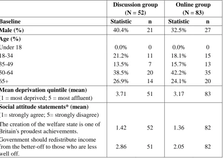
The first two samples had similar age and gender characteristics. Overall, the discussion
sample was slightly more affluent than the other two samples. Respondents in both the two
online groups were slightly more likely to have egalitarian social attitudes than respondents
in the discussion group.
3.2 The distribution of switching point by question and by sample
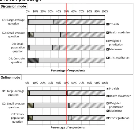
Figure 2 shows the distribution of responses across the five principles of health justice,
13
Figure 2: Inferred principles of health justice by question and sample design [about here]
Each stacked bar indicates the proportion of responses ranging from “pro-rich” on the left end
to “strict egalitarian” on the right end. As can be seen, in the first three questions, the median
respondent is “strong egalitarian” (i.e. “maximin” or “strict egalitarian”) in the discussion sample but is always “weighted prioritarian” in the online sample. However, the median
respondent in the discussion group sample shifts to “weighted prioritarian” in the concrete
question (this question was not used on the online sample).
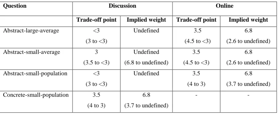
Table 3 presents the trade-off points of the median respondent and the implied equity weight
to the poorest fifth compared with the richest fifth. In general, the discussion group had lower
point estimates of median trade-off points; however, the confidence intervals (CI) of the
trade-off points in the discussion and online groups always included the strong egalitarian
trade-off point (3.0 or <3), and therefore the CI for the implied weights were undefined.
Table 3: Median response in different groups, with 95% confidence interval in brackets
[about here]
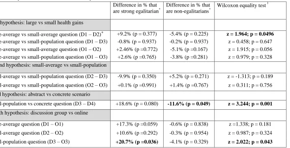
Table 4: Non-parametric statistical tests: all respondents [about here]
Table 4 shows the results of statistical tests for the hypotheses. We adopt a conservative
approach throughout and always reported two-sided tests. We use labels D and O for
discussion and online groups respectively. Hence, D1 represents Q1 in the discussion group,
and so forth.
Our first hypothesis was that small gains (small-average, Q2; and small-population Q3)
would yield less egalitarian responses than unrealistically large gains (Q1). We found that
the large-average and small-population questions gave similar results within both the
discussion (D1-D3) and online samples (O1-O3). On the other hand, responses were less
egalitarian in the small-average question compared with the large-average question.
However, this difference was not statistically significant in the online sample (O1-O2) and
only just reached statistical significance in one of the three tests within the discussion group
14
versus small gains comparisons – the largest difference was a 9.2 percentage point difference
in the proportion expressing strong egalitarian views (D1-D2). Overall, therefore, there was
no clear evidence of a substantial and systematic effect.
Our second hypothesis was that responses would be more egalitarian under population-level
(Q2) rather than individual-level (Q3) descriptions of the small gains question. The pattern
of responses was in this direction within the discussion group (D2-D3), but did not reach
statistical significance in any of the tests. Furthermore, there was no such pattern of
responses within the online sample (O2-O3). Again, therefore, there was no evidence of an
effect.
Our third hypothesis was that responses might differ (in either direction) between concrete
(D4) and abstract (D3) scenarios. In all three tests we found that discussion group sample
responses were significantly more egalitarian under the abstract rather than concrete scenario,
providing clear support for the third hypothesis.
Finally, our fourth hypothesis was that discussion group respondents (D) would be more
egalitarian than online respondents (O). This was indeed the general pattern of responses,
with a substantially larger proportion of the discussion group sample (between 11 and 21
percentage points) expressing strong egalitarian responses in all three questions. However,
only the small-population question (D3-O3) reached statistical significance. So this provides
some albeit weak support for our fourth hypothesis.
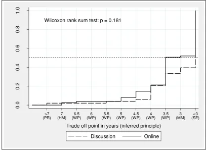
Figure 3 gives a visual representation of the rank-sum test, using the example of the
large-average question comparing the discussion versus online samples (D1 vs O1). Along the
horizontal axis are the 11 ranked points at which respondents can be indifferent between the
two programmes. The vertical axis represents the cumulative proportion of respondents who
have switched to the less egalitarian programme A by that point. The stronger the inequality
aversion, the lower the cumulative curve. In Figure 3, the cumulative curves are similar up to
4 but then the online group rises more rapidly showing a smaller proportion of respondents
giving the “strong egalitarian” responses of 3 (“maximin”) and <3 (“strict egalitarian).
15
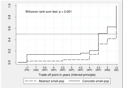
Figure 4 shows a cumulative rank comparison within the discussion group sample, comparing
abstract and concrete versions of the small-population presentation (D3 vs D4). This time the
curves start to diverge early on, with a higher proportion of <3 (“pro-rich”) and 3 (“health
maximiser”) responses under the concrete question frame.
Figure 4: Cumulative distribution of trade-off points for the small-population vs concrete question for the discussion group (D3 vs D4) [about here]
4. Discussion
A number of studies have attempted to quantify societal value judgements about equity,
including value judgements about severity and burden of illness, end of life, and health
inequality aversion (Rowen et al., 2016), (Linley and Hughes, 2013), (Shah et al., 2013,
Dolan and Tsuchiya, 2011). While these studies elicit public views, most do not evaluate the
effect of different scenario presentations and mode of administration that may influence the
final results. This paper contributes towards filling this gap in the context of health inequality
aversion, by performing experimental tests contrasting: (1) small instead of unrealistically
large health inequality reductions; (2) population-level instead of individual-level
descriptions of health inequality reductions; (3) concrete instead of abstract intervention
scenarios; and (4) online instead of face to face mode of administration.
We find no clear evidence of systematic and substantial effects of small versus unrealistically
large health inequality reduction scenarios (1) or population-level descriptions (2). However,
we do find clear evidence of an inequality aversion-reducing concrete scenario effect (3), and
weak evidence of an inequality aversion-reducing online mode of administration effect (4).
Within our discussion group sample, the proportion of non-egalitarians rose substantially and significantly when using a concrete rather than abstract scenario (by 12 percentage points), and the proportion expressing extreme inequality aversion fell substantially and significantly (by 19 percentage points). Finally, respondents were substantially more likely to give strict egalitarian responses in our discussion group sample compared with our online sample (by between 11 and 21 percentage points), although this pattern of findings only reached
16
Despite these three effects, however, median responses always implied substantial health inequality aversion and the implied weight to health gains in the worst off group never fell below 2.57 in any of our experimental conditions or sub-groups.
One possible explanation for the concrete scenario effect is that the intervention in question
(a reminder letter to promote uptake of bowel cancer screening) was an “agentic” intervention to promote individual health behaviour change, rather than a “structural”
intervention to alter the social determinants of health. “Agentic” interventions may make
concepts of individual responsibility for health behaviour and outcomes more salient in
respondents’ minds, thus reducing aversion to health inequality. If so, abstract scenarios may
tend to produce higher estimates of public concern for reducing health inequality than
concrete scenarios based on “agentic” interventions.
Finally, the mode of administration effect may suggest a “social desirability bias” whereby
face-to-face administration tends to elicit pro-egalitarian “Sunday best” responses. On the
other hand, the (slightly) less egalitarian social attitudes reported by the discussion group
sample suggests that this may be because face-to-face discussion provides a better
opportunity for careful deliberation. Either way, it is important that decision makers are
aware of the nature and magnitude of potential biases, so that they can appropriately assess
and interpret evidence about public views.
One of the considerations in inequality aversion surveys is the choice of terminology used to
describe the socioeconomic groups being compared. Our survey describes these groups as the
‘richest’ and ‘poorest’ fifth. This is both technically correct and easy to understand for the
participants. Other terms such as most/least deprived and most advantaged/disadvantaged
have been used in the literature. However, while the choice of terminology may influence the
point of indifference within a scenario description, it is unlikely that the effects found in our
study between scenario descriptions and between modes of administration may be due to the
choice of this terminology.
We note that a number of valuation tools exist to elicit equity-efficiency trade-offs (Gu et al
2015); these may or may not provide different estimates of inequality aversion. However, the
cognitive effects identified in our study are also likely to be relevant to other valuation tools.
17
used focus on health gains, and not the final distributions of health. In this respect, this study
may be criticised for favouring gain egalitarianism over outcome egalitarianism (Tsuchiya
and Dolan, 2009). However, since identical framing with a fixed ratio of gains has been
maintained across all questions, we expect this potential effect to cancel out in the
comparisons across pairs of questions that we carried out. Another potential criticism of the
study may be that respondents may favour the first (or the left hand side) option over the
second alternative in pair-wise comparisons (commonly known as ‘response order effect’);
similarly, the titration sequence in which questions are presented (compared to random order
presentation) may influence choice behaviour. However, Abasolo and Tsuchiya (2013)
specifically evaluated both effects and found no evidence of significant difference due to
response order or titration sequence.
Another potential criticism is that the order of questions was not randomised which may
influence value judgments due to a “learning effect”. However, we did not find a consistent
pattern of responses across questions to suggest such effect. Finally, we acknowledge that the
sample size of this study is relatively modest, although large enough to detect at least two
statistically significant effects. As a suggestion for future research in this area, we
recommend that the biases considered in this study should be investigated in larger samples.
Another consideration in this study is the generalisability of our findings from a small sample
to the general population. We think that while the absolute level of inequality aversion may
vary between population groups, the cognitive effects found in this study are likely to hold
true in other settings. However, further research is needed to investigate these biases in larger
and more diverse samples.
Overall, however, the basic finding of substantial health inequality aversion is surprisingly
robust. There was no substantial or clearly significant effect of using small rather than
unrealistically large health gains, or using population-level rather than individual-level
presentations. And although a concrete scenario and online mode of administration reduced
the proportion of respondents expressing infinite inequality aversion, median responses in all
18 References
ABASOLO, I. & TSUCHIYA, A. 2004. Exploring social welfare functions and violation of monotonicity: an example from inequalities in health. Journal of Health Economics, 23, 313-329.
ABÁSOLO, I. & TSUCHIYA, A. 2013. Is more health always better for society? Exploring public preferences that violate monotonicity. Theory and decision, 74, 539-563.
ASARIA, M., GRIFFIN, S., COOKSON, R., WHYTE, S. & TAPPENDEN, P. 2014. DISTRIBUTIONAL
COST EFFECTIVENESS ANALYSIS OF HEALTH CA‘E P‘OG‘AMMES A METHODOLOGICAL
CASE STUDY OF THE UK BOWEL CANCER SCREENING PROGRAMME. Health economics, DOI: 10.1002/hec.3058.
ASARIA, M., GRIFFIN, S., COOKSON, R., WHYTE, S. & TAPPENDEN, P. 2015. Distributional
C E A H C P A Methodological Case Study of the
UK Bowel Cancer Screening Programme. Health economics, 24, 742-754.
BLUMENTHAL-BARBY, J. & KRIEGER, H. 2014. Cognitive Biases and Heuristics in Medical Decision Making A Critical Review Using a Systematic Search Strategy. Medical Decision Making, 0272989X14547740.
BOWLING, A. 2005. Mode of questionnaire administration can have serious effects on data quality. Journal of public health, 27, 281-291.
DAMSCHRODER, L. J., ZIKMUND-FISHER, B. J. & UBEL, P. A. 2005. The impact of considering adaptation in health state valuation. Social science & medicine, 61, 267-277.
DEMAIO, T. J. 1984. Social desirability and survey measurement: A review. Surveying subjective phenomena, 2, 257-281.
DOLAN, P. & TSUCHIYA, A. 2011. Determining the parameters in a social welfare function using stated preference data: An application to health. Applied Economics, 43, 2241-2250.
GY‘D HANSEN D K‘ISTIANSEN I S P S
or gambling for the prize? Health economics, 17, 709-720. KAHNEMAN, D. 2011. Thinking, fast and slow, Macmillan.
KIM, S., GOLDSTEIN, D., HASHER, L. & ZACKS, R. T. 2005. Framing effects in younger and older adults. The Journals of Gerontology Series B: Psychological Sciences and Social Sciences, 60, P215-P218.
KRAGT, M. E. & BENNETT, J. W. 2012. Attribute framing in choice experiments: how do attribute level descriptions affect value estimates? Environmental and Resource Economics, 51, 43-59. KÜHBERGER, A. 1998. The influence of framing on risky decisions: A meta-analysis. Organizational
behavior and human decision processes, 75, 23-55.
LINLEY W G HUGHES D A S V O N C D F A V B
P C F P M A C S S O A I G
Britain. Health economics, 22, 948-964.
LOVE-KOH, J., ASARIA, M., COOKSON, R. & GRIFFIN, S. 2015. The Social Distribution of Health: Estimating Quality-Adjusted Life Expectancy in England. Value in Health, 18, 655-662.
MALENKA, D. J., BARON, J. A., JOHANSEN, S., WAHRENBERGER, J. W. & ROSS, J. M. 1993. The framing effect of relative and absolute risk. Journal of general internal medicine, 8, 543-548.
MCFADDEN, D. 2001. Economic choices. The American Economic Review, 91, 351-378.
MONGA, A. & BAGCHI, R. 2012. Years, months, and days versus 1, 12, and 365: the influence of units versus numbers. Journal of Consumer Research, 39, 185-198.
MULHERN, B., LONGWORTH, L., BRAZIER, J., ROWEN, D., BANSBACK, N., DEVLIN, N. & TSUCHIYA, A. 2013. Binary choice health state valuation and mode of administration: head-to-head comparison of online and CAPI. Value in Health, 16, 104-113.
NORMAN, R., HALL, J., STREET, D. & VINEY, R. 2013. Efficiency and equity: a stated preference approach. Health economics, 22, 568-581.
19
OLSEN, J. A. 2000. A note on eliciting distributive preferences for health. Journal of health economics, 19, 541-550.
PARK, A., BRYSON, C., CLERY, E., CURTICE, J. & PHILLIPS, M. 2013. British social attitudes 30, NatCen.
‘OD‘ÍGUEZ MÍGUEZ E PINTO P‘ADES J L M
concentration or dispersion of individual health benefits. Health economics, 11, 43-53. ROWEN, D., BRAZIER, J., MUKURIA, C., KEETHARUTH, A., HOLE, A. R., TSUCHIYA, A., WHYTE, S. &
SHACKLEY, P. 2016. Eliciting societal preferences for weighting QALYs for burden of illness and end of life. Medical Decision Making, 36, 210-222.
SCHWAPPACH, D. L. 2003. Does it matter who you are or what you gain? An experimental study of preferences for resource allocation. Health economics, 12, 255-267.
SHAH, K. K., COOKSON, R., CULYER, A. J. & LITTLEJOHNS, P. 2013. NICE's social value judgements about equity in health and health care. Health Econ Policy Law, 8, 145-65.
SKEDGEL, C. D., WAILOO, A. J. & AKEHURST, R. L. 2015. Choosing vs. allocating: discrete choice
preferences. Health Expectations, 18, 1227-1240.
20
21
Figure 2:
Inferred principles of health justice by question
and sample design * **
* Pro-rich (AAAAA); health maximiser (=AAAA); weighted prioritarian (BXXXA); Maximiner (BBBB=); Strict egalitarian (BBBBB)
22
Wilcoxon rank sum test: p = 0.181
0 .0 0 .2 0 .4 0 .6 0 .8 1 .0 >7 (PR) 7 (HM) 6.5 (WP) 6 (WP) 5.5 (WP) 5 (WP) 4.5 (WP) 4 (WP) 3.5 (WP) 3 (MM) <3 (SE)
Trade off point in years (inferred principle)
[image:23.595.122.532.96.393.2]Discussion Online
Figure 3:
Cumulative distribution of trade-off points for the large-average
question, by mode of administration (D1 vs O1)* **
* The trade off point represents the point at which the respondent would be indifferent between the less egalitarian programme A, in terms of the gain in years of life in full health to the poorest fifth in Programme B
23
Figure 4:
Cumulative distribution of trade-off points for the
small-population vs concrete question for the discussion group (D3 vs D4)
Wilcoxon rank sum test: p = 0.001
0
.0
0
.2
0
.4
0
.6
0
.8
1
.0
>7 (PR)
7 (HM)
6.5 (WP)
6 (WP)
5.5 (WP)
5 (WP)
4.5 (WP)
4 (WP)
3.5 (WP)
3 (MM)
<3 (SE)
Trade off point in years (inferred principle)
24
Table 1: Types of value judgement about health justice
Rank
(from pro-rich to strict egalitarian)
Types of view about health justice Trade-off point
1 Pro-rich (AAAAA) >7
2 Health maximiser (=AAAA) 7.0
3 Weighted prioritarian (BAAAA) 6.5
4 Weighted prioritarian (B=AAA) 6.0
5 Weighted prioritarian (BBAAA) 5.5
6 Weighted prioritarian (BB=AA) 5.0
7 Weighted prioritarian (BBBAA) 4.5
8 Weighted prioritarian (BBB=A) 4.0
9 Weighted prioritarian (BBBBA) 3.5
10 Maximin (BBBB=) 3.0
11 Strict egalitarian (BBBBB) <3
Table 2: Descriptive statistics of the discussion group and on-line survey respondents
Discussion group
(N = 52)
Online group (N = 83)
Baseline Statistic n Statistic n
Male (%) 40.4% 21 32.5% 27
Age (%)
Under 18 0.0% 0 0.0% 0
18-34 21.2% 11 18.1% 15
35-49 13.5% 7 15.7% 13
50-64 38.5% 20 42.2% 35
65+ 26.9% 14 24.1% 20
Mean deprivation quintile (mean)
(1 = most deprived; 5 = most affluent) 3.71 51 3.17 83 Social attitude statements* (mean)
(1= strongly agree; 5= strongly disagree)
The creation of the welfare state is one of
Britain's proudest achievements. 1.42 52 1.36 82
Government should redistribute income from the better-off to those who are less well off.
2.86 51 2.05 82
[image:25.595.75.513.349.659.2]25
Table 3: Median response in different groups, with 95% confidence interval in brackets
Question Discussion Online
Trade-off point Implied weight Trade-off point Implied weight
Abstract-large-average <3
(3 to <3)
Undefined 3.5
(4.5 to <3)
6.8
(2.6 to undefined)
Abstract-small-average 3
(3.5 to <3)
Undefined
(6.8 to undefined)
3.5
(4.5 to <3)
6.8
(2.6 to undefined)
Abstract-small-population <3
(3 to <3)
Undefined 3.5
(4 to 3)
6.8
(3.7 to undefined)
Concrete-small-population 3.5
(4 to 3)
6.8
(3.7 to undefined)
26 Table 4: Non-parametric statistical tests: all respondents
Difference in % that are strong egalitarian*
Difference in % that are non-egalitarians*
Wilcoxon equality test
First hypothesis: large vs small health gains
Large-average vs small-average question (D1 – D2)+ +9.2% (p = 0.377) -5.4% (p = 0.225) z = 1.964; p = 0.0496
Large-average vs small-population question (D1 – D3) -0.8% (p = 0.937) -0.2% (p = 0.937) z = 0.458; p = 0.647 Large-average vs small-average question (O1 – O2) +2.46% (p =0.772) -5.1% (p =0.167) z = 1.915; p = 0.056 Large-average vs small-population question (O1 – O3) +2.6% (p =0.765) -3.8% (p =0.281) z = 0.979; p = 0.328 Second hypothesis: small-average vs small-population
Small-average vs small-population question (D2 – D3) -9.9% (p = 0.350) +5.2% (p = 0.271) z = -1.313; p = 0.189
Small-average vs small-population question (O2 – O3) +0.1% (p =0.991) +1.4% (p =0.767) z = 0.311; p = 0.756
Third hypothesis: abstract vs concrete scenario
Small-population vs concrete question (D3 – D4) +18.6% (p = 0.080) -11.6% (p = 0.049) z = 3.244; p = 0.001
Fourth hypothesis: discussion group vs online
Large-average question (D1 – O1) +17.3% (p =0.059) -0.6% (p = 0.838) z =1.338; p = 0.181
Small-average question (D2 – O2) +10.6% (p =0.292) -0.3% (p = 0.954) z = 0.987; p = 0.324
Small-population question (D3 – O3) +20.7% (p =0.036) -4.1% (p = 0.329) z = 2.022; p = 0.043
* Strong egalitarians = maximiner or strict egalitarian; Non-egalitarians = pro-rich or health maximisers. p-values provided for test of equality of proportions. * Negative sign indicates less egalitarian (or non-egalitarian in the third column) in the first group compared to the second group, and vice versa.
Wilcoxon rank-sum test was used for unmatched data and signed-rank test was used for matched data. Null hypothesis: two samples are from populations with the same distribution.
27 APPENDICES
APPENDIX 1:
Estimating the inequality aversion parameter
To estimate health inequality aversion parameters, one can use a symmetric social welfare
function with constant elasticity of substitution (CES):
where W is the level of health related social welfare; Hi(≥ 0) is the level of years of life in
full health for population group i, where i = R for the richest fifth and i = P for the poorest
fifth; and r (≥ -1, ≠ 0) is the inequality aversion parameter. When a respondent is indifferent
between two programmes A and B, these two outcomes are on the same social welfare
contour. At the mid-point of A and B, the gradient of the contour is:
which is also (approximately) equal to:
From this relationship, a unique value of r can be obtained, either mathematically (Abasolo
and Tsuchiya, 2004) or by using the solve tool in a spread sheet (Dolan and Tsuchiya, 2011).
Once the value of r is obtained, the implied equity weight given to a marginal improvement
in the health of the poorest fifth relative to the health of the richest fifth can be calculated
28
Appendix Table 1: Calculation table to estimate the inequality aversion parameter of a symmetric social welfare function with constant elasticity of substitution for the large-average question (source: Abasolo and Tsuchiya 2004)
Types of preference (choice behaviour)
Trade-off point
QALE* of the rich (Prog A)
QALE of the rich (Prog B)
QALE of the poor (Prog A)
QALE of the poor (Prog B)
Inequality aversion parameter
Implied weight
1 Pro-rich (AAAAA) >7 81 77 65 Undefined [**] [**]
2 Health maximiser
(=AAAA) 7.0 81 77 65 69 -1.00 1.00
3 Weighted prioritarian
(BAAAA) 6.5 81 77 65 68.5 -0.21 1.15
4 Weighted prioritarian
(B=AAA) 6.0 81 77 65 68 0.67 1.34
5 Weighted prioritarian
(BBAAA) 5.5 81 77 65 67.5 1.67 1.60
6 Weighted prioritarian
(BB=AA) 5.0 81 77 65 67 2.86 1.98
7 Weighted prioritarian
(BBBAA) 4.5 81 77 65 66.5 4.34 2.57
8 Weighted prioritarian
(BBB=A) 4.0 81 77 65 66 6.40 3.70
9 Weighted prioritarian
(BBBBA) 3.5 81 77 65 65.5 9.87 6.85
10 Maximin (BBBB=) 3.0 81 77 65 65 Undefined Undefined
11 Strict egalitarian
(BBBBB) <3 81 77 65 Undefined Undefined Undefined
* QALE: Quality adjusted life expectancy