White Rose Research Online URL for this paper:
http://eprints.whiterose.ac.uk/126299/
Version: Accepted Version
Article:
Checco, A. orcid.org/0000-0002-0981-3409 and Leith, D.J. (2017) Fast, responsive
decentralized graph coloring. IEEE/ACM Transactions on Networking, 25 (6). pp.
3628-3640. ISSN 1063-6692
https://doi.org/10.1109/TNET.2017.2751544
© 2017 IEEE. Personal use of this material is permitted. Permission from IEEE must be
obtained for all other users, including reprinting/ republishing this material for advertising or
promotional purposes, creating new collective works for resale or redistribution to servers
or lists, or reuse of any copyrighted components of this work in other works. Reproduced
in accordance with the publisher's self-archiving policy.
[email protected] https://eprints.whiterose.ac.uk/ Reuse
Unless indicated otherwise, fulltext items are protected by copyright with all rights reserved. The copyright exception in section 29 of the Copyright, Designs and Patents Act 1988 allows the making of a single copy solely for the purpose of non-commercial research or private study within the limits of fair dealing. The publisher or other rights-holder may allow further reproduction and re-use of this version - refer to the White Rose Research Online record for this item. Where records identify the publisher as the copyright holder, users can verify any specific terms of use on the publisher’s website.
Takedown
If you consider content in White Rose Research Online to be in breach of UK law, please notify us by
Fast, Responsive Decentralised Graph Colouring
Alessandro Checco and Doug J. LeithAbstract—Graph colouring problem arises in numerous networking applications. We solve it in a fully decentralised way (i. e.with no message passing). We propose a novel algorithm that is automatically responsive to topology changes, and we prove that it converges to a proper colouring inO(NlogN)time with
high probability for generic graphs when the number of available colours is greater than∆, the maximum degree of the graph, and inO(logN)time if∆ =O(1). We believe the proof techniques
used in this work are of independent interest and provide new insight into the properties required to ensure fast convergence of decentralised algorithms.
I. INTRODUCTION
Many fundamental wireless network allocation tasks can be formulated as a colouring problem, including channel and sub-carrier allocation [8], TDMA scheduling [1, 9], scrambling code allocation [6], network coding [8] and so on. Importantly, these tasks must often be solved while respecting strong communication constraints due, for example, to the range over which devices can communicate being smaller than the range over which they interfere or otherwise interact. Moreover, the network topology can change over time, re-quiring the nodes to dynamically adapt to this. Recently, fully decentralised Communication-Free Learning (CFL) algorithms have been proposed for solving general constraint satisfaction problems without the need for message-passing [8] and with the ability to respond automatically to topology changes. These Communication-Free Learning (CFL) algorithms ex-ploit local sensing to infer satisfaction/dissatisfaction of con-straints, thereby avoiding the need for message-passing and use stochastic learning to converge to a satisfying assignment. The extension to colouring problems with strong sensing restrictions is investigated in [5].
However, this class of algorithms has not been proven to be fast: the only analytic bound available is exponential in the number of nodes. Further, even though the performance observed in simulations is typically sub-exponential, the de-pendency of the convergence rate on the algorithm parameters is not clear.
In this paper we address both of these issues. We propose a novel algorithm that is provably fast (O(NlogN)when the number of available colours is greater than ∆(the maximum degree of the graph). Moreover, this algorithm is well suited to implementation on resource constrained devices such as RFID tags, because it has a small memory and computation footprint, involves no floating point arithmetic, no multiplications or
A. Checco is with the Information School, University of Sheffield, UK. Email: [email protected].
D.J. Leith is with the School of Computer Science and Statistics, Trinity College Dublin, Ireland. Email: [email protected]
This work was supported by Science Foundation Ireland under Grant No. 11/PI/1177.
Manuscript received October 27, 2015; revised September 1, 2017.
divisions and only needs the availability of a uniform random number generator. The algorithm makes use of a new type of “memory” when learning a colouring and this gives some insight into which parts of the existing stochastic learning algorithms are needed to ensure fast convergence. We analyse how the algorithm parameters affect the convergence rate, and determine choices that guarantee fast convergence while maintaining responsiveness to topology changes.
Our theoretical bounds on convergence rate are obtained using a novel stochastic drift analysis that we believe is of independent interest.
A. Related Work
In the graph theory and computer science literature, the problem of colouring with∆ + 1colours has been thoroughly studied [12, 15, 17, 21]. In particular, the family of locally iterative algorithmshas received much attention. This family of algorithms makes use of the following strong assumptions: 1) The algorithm can use an unbounded number of colours during its operation, although it eventually reduces the number over time;
2) The graph topology is assumed to be known and fixed; 3) Each graph vertex needs to know which colours are used
by its neighbours.
Szegedy and Vishwanathan [21] use an heuristic argument to show that no locally iterative (∆ + 1)-colouring algorithm is likely to terminate in less than Ω(∆ log ∆) rounds (lower bound). More refined bounds have been obtained in [3, 11].
However, in the wireless networking field, these three assumptions are rarely satisfied. To our knowledge, Assump-tion 1 is not used by any work in the wireless networking field, presumably because it is obviously inappropriate for such applications. Assumption 2 has been relaxed in two main ways: by using network-wide stopping/restarting techniques in annealing-like algorithms [13], and by use of learning algorithms [2, 4, 8, 14, 15, 21]. Assumption 3 (in the form of either centralised or gossiping-like message passing) is used in [7, 12, 13, 20, 23]. However, communication between nodes often cannot be relied upon in the design of a robust algorithm in cases wheree. g.wireless nodes belong to different admin-istrative domains or when the devices are too simple to be able to realise such communication (see, for example, Radio-Frequency Identification devices).
The most challenging problem of graph colouring in which no message passing is possible (so none of the three assump-tions hold) has recently attracted attention in the wireless networking literature in [2, 8, 18].
The Learning-BEB algorithm, proposed by Barcelo et al. [2] is an algorithm devised for achieving collision-free scheduling in 802.11 networks. It is a modification of the CSMA/CA
mechanism of truncated exponential backoff: after a successful transmission, the transmitter uses a fixed backoff interval
P, while after a collision it selects an interval uniformly at random (u.a.r.) in the contention window range. Within the terminology of graph theory, this corresponds to a colouring algorithm in which each node selects the same colour after being locally satisfied, and selects a colour u.a.r. otherwise. This algorithm is known to suffer from slow convergence rates [9], but it has the advantage of being easy to implement. Roughly speaking, for a complete graph the probability of success for the whole graph in a step is (1/N)N. So, the
number of iterations needed to completely colour a graph with this method with probability bigger than1−ǫis of the order oflog(ǫ−1)e(N logN), that is exponential in N.
The algorithm proposed by Motskin et al. [18] is similar to [2], with the advantage of being provably fast (O(logN)
when ∆ = O(N)) but with the major disadvantage of not being adaptive to topology changes, since after a correct local choice, the node keeps the chosen colour forever. The possibility of change in topology, together with the constraint of no message passing, makes this algorithm unable to ”reset” when a change of topology happens, and thus this intuitive approach does not work.
The CFL algorithm proposed by Duffy et al. [8] uses a stochastic learning mechanism to update the probability of choosing each colour based on local sensing. In simulations it is fast, and it is provably adaptive to topology changes. The main disadvantage is that it is hard to prove good convergence rate bounds and it is too complicated to implement in simple hardware such as Radio-Frequency Identification (RFID) tags. It is worth noting that all three algorithms share the common property of initially selecting colours u.a.r. and staying with the same colour when locally satisfied. They also all belong to the family of locally iterative algorithm, even if they do not use assumptions 1-3. The difference between them lies in the way they respond to a loss of local satisfaction: Learning-BEB will go back to u.a.r. selection, the algorithm proposed by Motskin et al. [18] will keep the same choice even if locally unsatisfied, and CFL will distribute the probability mass amongst all colours, decreasing the probability of choosing the current un-satisfying colour. Learning-BEB is equivalent to CFL when the latter uses parametersa=b= 1(in the terminology of [8]).
To summarise, when message passing is not allowed and the graph topology can change over time, the existing solutions cannot provide a provably fast colouring, because of one of these reasons:
• The ability to react to a topology change creates conver-gence speed problems (Learning-BEB [2]).
• The ability to quickly converge comes at the expense of being unable to react to topology changes (algorithm in [18]).
• The ability to learn from the local graph topology by passive observation of the local state of a vertex via stochastic mechanisms make very arduous to prove fast convergence (CFL [8]).
Our approach allows to gain some insight into which parts of the existing stochastic learning algorithms are needed to
ensure fast convergence, so that a simple and provably fast algorithm can be devised.
II. PRELIMINARIES: PROBLEMDEFINITION
We use the notation introduced in [8] for the more general decentralised constraint satisfaction problem, applying it to graph colouring problem as in [5].
Let G = (N,E) denote an undirected graph with set of vertices N = {1, . . . , N} and set of edges E := {(i, j) : i, j ∈ N, i ↔j}, where i↔ j denotes the existence of an edge betweeniand j. Let ∆denote the maximum degree of vertices in graphG i. e.the maximum number of neighbours. A Colouring Problem (CP) on graphG with D∈N colours
is defined as follows. Let xi∈ Ddenote the colour of vertex
i, whereD={1, . . . , D}is the set of available colours, and
~x denote the vector(x1, . . . , xN). Define clauseΦm:DN 7→
{0,1} for each edgem= (i, j)∈ E with:
Φm(~x) = Φm(xi, xj) =
(
1 ifxi6=xj
0 otherwise.
We say clause Φm(~x)issatisfied if Φm(~x) = 1. An
assign-ment~xis said to be satisfying if for all edgesm∈ E we have
Φm(~x) = 1. That is
~x is a satisfying assignment iff min
m∈EΦm(~x) = 1. (1)
Equivalently,~x is a satisfying assignment if and only ifxi6=
xj for all edges (i, j) ∈ E i. e. if i ↔ j. For any colour
allocation, we say a vertex isunsatisfied if at least one of its neighbours has the same colour; otherwise the vertex is said to besatisfied. A satisfying assignment for a colouring problem is also called aproper colouring.
Definition 1 (Chromatic Number). The chromatic number
χ(G)of graphG is the smallest number of colours such that at least one proper colouring of Gexists.
We require the number of colours D in our palette to be greater than or equal to χ(G) for a satisfying assignment to exist.
A. Decentralized CP Solvers
Definition 2 (CP solver). Given a CP, a CP solver realizes a sequence of vectors{~x(t)}such that for any CP that has a satisfying assignment
(D1) for allt sufficiently large~x(t) =~x for some satisfying assignment ~x;
(D2) if t′ is the first entry in the sequence{~x(t)} such that
~x(t′)is a satisfying assignment, then~x(t) =~x(t′)for all
t > t′.
In order to give criteria for classification of decentralized CP solvers, we re-write the LHS of Equation (1) to focus on the satisfaction of each variable
~x is a satisfying assignment iff min
i∈Nmmin∈Ei
Φm(~x) = 1. (2)
whereEi consists of all edges in E that contain vertexi,i. e.
A decentralized CP solver is equivalent to a parallel solver, where each variablexiruns independently an instance of the
solver, having only the information on whether all of the clauses thatxiparticipates in are satisfied or at least one clause
is unsatisfied. The solver located at variablexi must make its
decisions only relying on this information.
Definition 3 (Decentralized CP solver). A decentralized CP solver is a CP solver that for each variablexi, must select its
next value based only on the evaluation of
min
m∈Ei
Φm(~x). (3)
That is, the decision is made without knowing
(D3) the assignment ofxj forj6=i.
(D4) the set of clauses that any variable, including itself, participates in, Ej forj∈ N.
(D5) the clausesΦm form∈ E.
III. FASTCOLOURING
The basic idea used in [8] to establish convergence is to show that (i) for any graph and starting from any choice of colours there exists a sample path that leads to a proper colouring and (ii) overO(N)iterations this sample path occurs with probability bounded away from zero. While providing a bound on the convergence rate that appears to be order optimal, this approach cannot be used to show that fast convergence occurs when the number D of colours is at least ∆ + 1. For that, we need an approach that provides insight into how the fraction of sample paths leading to a proper colouring
increaseswithD. In this paper we therefore adopt an entirely different approach from that in [8], namely one based on stochastic drift analysis.
A. FCFL Algorithm
As will become clear, it will prove helpful to consider the following generalisation of the CFL algorithm, called Fast Communication-Free Learning (FCFL):
Algorithm 1 Fast Communication-Free Learning 1: DefineSτ ∈N,τ = 1,2, . . . withSτ+1≥Sτ
2: Define D, the number of colours, parameter 0 < b≤ 1
and vectorp∈[0,1]D
3: Initialisep= D11,m= 0, countersτ = 1,t= 1
4: repeat
5: ift=Sτ then
6: τ =τ+ 1,m= 0 ⊲Reset, exit permanent state
7: end if
8: Select colourcwith probabilitypc
9: ifm= 0then
10: ifSatisfied then
11: p=δc ⊲ Stick with same colour
12: m= 1 ⊲Enter permanent state
13: else
14: p= (1−b)p+ Db1 ⊲Unsatisfied
15: end if
16: end if
17: t=t+ 1 18: untilForever
Each vertex maintains a vectorp∈[0,1]D, whereD is the
number of available colours, and a state m ∈ {0,1}. When
m= 1the vertex is said to be in thepermanentstate. Time is slotted with slots indexed byt= 1,2,· · ·. A copy of the FCFL algorithm is run by every vertex, which determines vectorp
and state m at each time slot. State mis initially 0, and is also reset to 0 at times Sτ,τ = 1,2, . . .. When m = 0, at
each time slot a vertex selects a colourc with probabilitypc
(thec’th element of vectorp). If none of its neighbours have selected the same colour, the vertex is said to be satisfied
and (i) p is updated so that all elements are 0 except for element pc which is set equal to1, (ii) the vertex enters the
permanent statem= 1. The vertex will therefore continue to select colour cuntil the next reset time1 S
τ. However, if one
or more neighbours have selected the same colour then the vertex updatesp to (1−b)p+ b
D1, reducing the probability
with with colourc is chosen, and tries again.
Evidently FCFL satisfies requirements D2-D5 of a CP solver, and we consider requirement D1 shortly. FCFL in-cludes CFL and the related algorithms in [2, 18] as special cases. When Sτ = τ, so that the state m is reset to 0 at
every time step, then FCFL is equivalent to CFL2. When, in addition, b = 1 then unsatisfied vertices select colours uniformly at random (pequals D11) and FCFL is equivalent to that considered in [2]. WhenS1→ ∞and b= 1 then FCFL is equivalent to that in [18] (unsatisfied vertices select colours uniformly at random and once satisfied a vertex then sticks with the same colour forever).
Intuitively, parameterbaffects the memory in the algorithm. For example, suppose a vertex has selected colour c and been satisfied so that pc = 1 but has subsequently become
unsatisfied (one of its neighbours has selected colourc). When
bis small, thenpc reduces only slowly and so the vertex will
tend to retry colourcrepeatedly. Conversely, whenb= 1then
pc is immediately reset to1/Dand becomes as equally likely
as any other colour to be selected at the next time slot. The interval Sτ+1−Sτ between reset times similarly affects the
rate of adaptation. When this interval is large then a vertex that has been satisfied keeps trying the same colour even when it becomes unsatisfied, and conversely when the interval is small. We will discuss the impact of b and Sτ on the convergence
rate in more detail below.
B. Absorbing State and Dynamic Recolouring
Observe that the FCFL algorithm involves no stop-ping/restarting but a proper colouring is an absorbing state for FCFL, corresponding to a situation where all vertices are satisfied i. e.once all vertices are satisfied then their colours will remain fixed. Importantly, the situation where all vertices are in the permanent state is also absorbing:
1Note that the permanent state differs from the satisfied and unsatisfied
states because a permanent vertex is guaranteed to be satisfied only at the round in which it becomes permanent.
2We found that the key difficulty with establishing the fast convergence of
Lemma 1 (Absorbing States). If all vertices are in the permanent state, then they are all satisfied.
Proof: First let us note that in the first round in which a vertex becomes permanent, it is satisfied and it cannot cause dissatisfaction to its neighbours; the neighbours can still be unsatisfied, but only because of other vertices. By contradiction, assume all vertices are in permanent state but there is at least one vertex i unsatisfied. So there must be at least another neighbour j unsatisfied and with same colour of i, by symmetry of dissatisfaction sensing. Now let us call
ti, tj the (last) time in which i and j became permanent,
respectively. Assume, w.l.o.g. thatti< tj (note that equality
is not possible, because at first round a vertex becomes permanent it is necessarily satisfied). Now at timetj,jbecame
permanent, so it chose a colour different from i, causing a contradiction.
It will also prove useful later to note the following:
Corollary 1. A vertex in the permanent state can be unsatis-fied only by non-permanent neighbours.
Observe also that a useful feature of the FCFL algorithm (and of CFL for that matter) is that should the graph subse-quently change, for example upon the appearance of a new vertex, such that the colouring is no longer proper then one or more vertices are not satisfied and these will automatically restart searching for a proper colouring after the next reset timeSτ+1has been reached. That is, there is no need for a co-ordinated restart with its associated communication overhead.
C. Convergence
Basic convergence of the FCFL algorithm can be shown an approach similar to that used in [8] for the CFL algorithm. Namely, we have:
Theorem 1(Convergence). Consider a feasible CP on a graph
G ={N,E}, with palette D. Suppose the FCFL reset times satisfy Sτ+1−Sτ ≤ M,τ = 1,2,· · · and S1 ≤ M. Given
any unsatisfied assignment of colours ~x(0)∈ DN, then with
probability greater than1−ǫ∈(0,1), the number of iterations for the FCFL algorithm to find a proper colouring is less than
M Nexp(M N(2N+1)log(D)) log(ǫ−1).
Proof: See Appendix.
However, while we know that FCFL converges, the bound on the convergence rate in Theorem 1 is not sufficient to establish fast convergence when the number of colours is ∆ + 1 or greater.
D. Outline of Drift-based Analysis
Let the random variableZt denote the number of vertices
which are not in the permanent state at time t. Recall that, by Lemma 1, Zt = 0 is an absorbing state. Letting R ∈
{1,2,· · · }be the earliest time such thatZR= 0. SinceZt is
integer valued it follows that P(R > t) =P(Zt ≥1) and by
Markov’s inequality,
0≤P(Zt≥1)≤E[Zt].
N = 2 N = 3 N = 4 N = 5 N = 6 N = 7
NumberZtof non-permanent vertices
E
[
Zt
+
1
|
Zt
]
−
Zt
0 1 2 3 4 5 6 7
[image:5.595.325.517.87.239.2]−3 −2.5 −2 −1.5 −1 −0.5 0 0.5 1
Fig. 1: Expected change in number of non-permanent vertices vs current number of non-permanent vertices. Results are shown for a complete graph withN vertices,D= ∆ + 1 =N
colours and the FCFL algorithm with parameters Sτ = τ,
b= 1.
Hence, it is sufficient to show that E[Zt] → 0 in order to
ensure that P(Zt ≥1) →0 and so P(Zt= 0) →1. Further
the convergence time ofE[Zt]upper bounds the convergence
time ofP(Zt≥1).
If we could show that at all timestthe driftEZt+1|Zt−
Zt≤ −ǫfor someǫ >0then this would be enough to ensure
thatE[Zt] decreases monotonically with time and also allow
the convergence rate to be upper bounded. Indeed, this is the approach taken in [18] in the special case of FCFL where
S1→ ∞.
Unfortunately, this approach cannot be used more generally since when the reset timesSτ are finite then the drift may, in
fact, be positive at these times i. e.the number of vertices in the permanent state can decrease. Further, this positive drift is essential to ensure that the algorithm is able to respond to changes (such as addition of new vertices) in the graph which require recolouring of vertices. Figure 1 illustrates this, showing the expected change in the number of non-permanent vertices vs the current number of non-permanent vertices for a complete graph (each vertex is connected to every other vertex, so the degree ∆ is N−1). For N >3 it can be seen that the drift is positive as the number of non-permanent vertices becomes small. This is quite intuitive: suppose two vertices are in the non-permanent state and so unsatisfied. Only in the relatively unlikely event in which they choose the remaining two available colours will the system converge to a proper colouring, otherwise the non-permanent vertices will cause one or more of the permanent vertices to be unsatisfied and so to exit the permanent state at the next reset time.
With the foregoing in mind, letS := {Sτ :τ = 1,2, . . .}
denote the set of the reset times when the FCFL algorithm allows vertices to exit the permanent state, and S¯:= N\ S
denote all other times. What we have is that at times t ∈S¯
the driftEZt+1|Zt−Zt must be non-positive (vertices can
enter the permanent state but cannot leave it) but at times
t∈ Sthe drift may be positivei. e.EZt+1|Ztmay increase.
time t
E
[Zt |Z1
]
[image:6.595.79.262.83.227.2]S1 S2
Fig. 2: Illustrating evolution ofE[Zt|Z1]vs time t. At times
t ∈ S the drift may be positive and the value may increase compared to timet−1∈S¯. Nevertheless, at the subsequence of times t ∈ S the net effect is forE[Zt|Z1] to decrease as
indicated by the dots on the dashed line.
convergence ofE[Zt]what we would like to show is thatE[Zt]
decreases monotonically at the sequence of reset timest∈ S, as indicated by the dots on the dashed line in Figure 2. But of course we want more than to just show convergence, we want to showfastconvergence and this requires tight control of the upper bound indicated by the dashed line so that it decreases sufficiently quickly.
E. Main Result – Fast colouring with∆ + 1 colours
We present the proof in the next section, but using the approach outlined above we can show that if at least ∆ + 1
colours are available (where ∆ is the maximum degree of the graph), FCFL is provably fast. That is it converges to a proper colouring in O(NlogN) time with high probability for any graph, and in O(logN) time for graphs of small maximum degree, i. e. graphs where ∆ = O(1). Moreover, this is achieved while keeping the intervalSτ+1−Sτ between
reset times small (∆ + 1), allowing the algorithm to respond quickly to topology changes.
Theorem 2 (Fast Convergence). Consider a CP on a graph
G = {N,E} with maximum degree ∆ and suppose that we have D > ∆ + 1 available colours. Let N := |N | ≥2 and
Zt be the set of vertices in the non-permanent state at time
t ∈ {0,1,2, . . .}, with |Zt| = Zt ∈ {0,1,2, . . . , N}. Let τ∗
index the first timeSτ∗ at which a proper colouring is found. For FCFL withSτ+1−Sτ ≥∆ + 1andb= 1we have
P τ∗≥B(N,∆, ǫ)
≤ǫ,
where
B(N,∆, ǫ) := logN+ log (ǫ
−1) +K
(∆ + 1) log∆+1 ∆ +
K
∆+1
andK = log1+2 log 21 .
Observe that Theorem 2 states the convergence rate in terms of the reset times Sτ. When we have Sτ+1−Sτ ≤M then
we can immediately express the convergence rate in terms of time slots.
Corollary 2. LetR∈ {1,2,· · · }be the earliest time such that graphGis properly coloured. When∆+1≤Sτ+1−Sτ ≤M,
τ = 1,2,· · · andS1≤M,b= 1then for FCFL
P R≥MlogN+O(1)≤ǫ, asN→ ∞.
Proof: Since Sτ+1−Sτ ≤ M for all t = 1,2,· · · and
S1≤M, we can bound the convergence rate in terms of time slots, namelyM B(N,∆, ǫ). Taking the limit ofM B(N,∆, ǫ)
asN,∆→ ∞ ends the proof.
Corollary 3 (Small degree). When Sτ = τ(∆ + 1), τ =
1,2,· · · (periodic reset times),b= 1and∆ =O(1), then for FCFL the convergence timeR=O(logN)asN→ ∞.
Proof: The thesis follows as for Corollary 2, by setting
M = ∆ + 1and assuming∆≤β.
Corollary 4(Almost complete graphs).WhenSτ =τ(∆+1),
τ = 1,2,· · ·, b = 1 and ∆ = Θ(N), then for FCFL the convergence time R=O(NlogN)asN→ ∞.
Proof: The thesis follows as for Corollary 2, by setting
M = ∆ + 1and assuminglimN,∆→∞∆N =β >0,.
A convergence time of O(NlogN) with ∆ + 1 colours is surprisingly close to that of the state-of-the-art given the constraints imposed by the decentralised nature of the FCFL algorithm. Faster convergence has recently been demonstrated (O(∆) +1
2log∗N [4]), but only for algorithms which (i) start with a much larger number of colours and then proceed to prune these until only∆ + 1 are used, (ii) require knowledge of the graph topology and (iii) make extensive use of message passing. Recall that FCFL imposes none of these requirements, and is therefore much better suited to networking applications. In Szegedy and Vishwanathan [21] it is argued that no locally-iterative (∆ + 1)-colouring algorithm is likely to terminate in less than Ω(∆ log ∆) rounds, implying that the FCFL algorithm may in fact be order optimal amongst locally-iterative algorithms in the case of complete graphs (when
∆ =N).
We note that Theorem 2 requires parametersSτ+1−Sτ ≥
∆ + 1 and b = 1 in the FCFL algorithm. We discuss the analytic difficulty which is the source of this requirement in more detail in the next section, but this is circumvented by the introduction of the permanent state and reset times in FCFL. As already noted, the permanent state introduces memory into the FCFL algorithm which bears qualitative similarities to that introduced in CFL by selecting parameter b to have a small value (typically 0.1 in [8]). This is of interest in its own right, quite apart from the resulting provably fast convergence, as it significantly broadens the class of known decentralised algorithms for graph colouring.
Further, this new approach is particularly amenable to highly efficient implementation, making it suited to use of resource constrained hardware such as RFID tags and sensors. For example, selecting a constant reset time Sτ = τ(∆ + 1)
Algorithm 2 Simplified Fast Communication-Free Learning 1: Initialise countert= 0
2: Select a colour uniformly at random 3: repeat
4: ift= 0then
5: t= ∆ + 1,m= 0 ⊲Reset, exit permanent state
6: end if
7: ifm= 0then
8: ifSatisfied then
9: m= 1 ⊲Enter permanent state
10: Leave colour unchanged.
11: else
12: Select a colour uniformly at random
13: end if
14: else
15: Leave colour unchanged.
16: end if
17: t=t−1 18: untilForever
Observe that this simplified FCFL algorithm involves no floating point arithmetic, no multiplications or divisions and only needs the availability of a uniform random number generator (which can be efficiently implemented in pseudo-random form).
IV. ANALYSINGCONVERGENCERATE
To proceed, for each vertex i ∈ N and each time t = 1,2, . . . define the random variable,
Xi(t) =
(
1, if vertexiis permanent at timet 0, otherwise.
LettingZt={i:Xi(t) = 0}denote the set of non-permanent
vertices at timetthenZt=|Zt|, the cardinality ofZt. Now,
EZt+1|Zt=Z= X
Z:|Z|=Z,
Z⊂N
(Φt(Z) + Ψt(Z))P Z|Zt =Z,
where
Φt(Z) :=E
X
i∈Z
(1−Xi(t+ 1))|Zt =Z
Ψt(Z) :=E
X
i∈N \Zt
(1−Xi(t+ 1))|Zt =Z
.
Suppose, for now, that we have bounds Φt(Z) ≤ φt(Z),
Ψt(Z)≤ψt(Z)whereZ =|Z|. That is, Φt(Z)andΨt(Z)
can be upper bounded by functions which depend only on the cardinality of setZ. Then it follows that,
E
Zt+1|Zt=Z≤φt(Zt) +ψt(Zt).
Recall S:={Sτ :τ = 1,2, . . .} is the set of the reset times
when the FCFL algorithm allows vertices to exit the permanent
state, andS¯:=N\ S. For slotst∈S¯vertices cannot exit the
permanent state and so ψt(Z) = 0. Hence,
EZt+1|Zt≤
(
φt(Zt) t∈S¯
φt(Zt) +ψt(Zt) t∈ S.
In order to streamline the discussion, and because they are satisfied by the FCFL algorithm, we make the follow-ing assumptions: (i) φt(·) is linear and time-invariant i. e.
φt(Z) =aZ with a≥0 and (ii) ψt(·)is concave. For slots
t∈S¯we then have,
EZt+1=EhEZt+1|Zti≤Eφt(Zt)(=a)φt(E[Zt])
where (a) follows sinceφt(·)is linear. Hence,
E[Z2]≤φ1(E[Z1])
E[Z3]≤φ2(E[Z2])≤φ2(φ1(E[Z1]))
and
EZS
1
≤φ(S1−1)(E[Z
1]), (4)
where φ(t)(Z) := φ
t ◦ · · · ◦φ1(Z) and ◦ denotes function compositioni. e.φt+1◦φt(Z) =φt+1(φt(Z)). This simplifies
to φ(t)(Z)≤αtZ under the assumption thatφ(·)is linear.
Now,
E
ZS1+1
≤E
φ(ZS1)
+E
ψS1(ZS1)
(b)
≤ φ(E
ZS1
) +ψS1(E
ZS1
) ≤αS1E[Z
1] +ψS1(α
S1−1E[Z
1]), where (b)follows since ψ(·) is concave. Hence, once again using the assumption thatφ(·)is linear,
E
ZS2+1
≤αS2E[Z1] +ψS 2(α
S2−S1−1ψ S1(α
S1−1E[Z1])), (5)
and we can repeat to obtain E
ZSτ+1
for τ = 1,2, . . .. However, it can be seen that the term involving ψt(·) in
the expression for E
ZSτ+1
quickly becomes complex and messy. It is precisely this term which captures the positive drift at timest∈ Sand which, as noted previously, makes the analysis tricky. The key insight underlying our analysis here is that in the case of the FCFL algorithm this term can be successfully controlled via a upper bound which is tractable yet tight enough to allow fast convergence to be established.
A. Bounding Φt(Z)for FCFL
Recall thatΦt(Z) is the expected number of vertices that
remain in the non-permanent state at timetconditioned on the set of non-permanent vertices beingZ. The probability that a vertex leaves the non-permanent state is characterised by the following lemma:
Lemma 2 (Entering Permanent State). We have that
P Xi(t+ 1) = 1|Xi(t) = 0 is the probability that a vertex
i which is in the non-permanent state at time t enters the permanent state at time t+ 1. When the number of colours
D≥∆ + 1then,
P Xi(t+ 1) = 1|Xi(t) = 0≥α:= b
Proof: A non-permanent vertex has at least D − ∆
available colours, and its choice is uniform, so it has a probability at least equal to b(D−D∆) to choose a colour not used by any neighbour. Now ∆D ≤ ∆+1∆ , becauseD≥∆ + 1; so we haveb(DD−∆) =b(1− ∆
D)≥b(1−∆+1∆ ) = ∆+1b . Lemma 2 is intuitive. By design, in FCFL the probability that a non-permanent vertex selects a colour is at least b/D
i. e. every colour has a uniformly lower bounded chance of being selected. When the number of coloursD≥∆ + 1then there is always at least one choice of colour different from that of every neighbour (since there can be at most∆neighbours). Selecting this colour will cause the vertex to become satisfied and enter the permanent state. Note that when b = 1 this bound is tight, i. e. there exists a degree∆ + 1 graph and a configuration of D = ∆ + 1 vertex colours for which it is satisfied with equality.
It follows from Lemma 2 that,
Φt(Z) =E
X
i∈Z
(1−Xi(t+ 1))|Zt=Z
=Z−E
X
i∈Z
Xi(t+ 1)|Zt =Z
≤Z−αZ= ∆ + 1−b
∆ + 1 Z=:φ(Z). (6)
Observe thatφ(Z)in (6) is linear inZ and time-invariant, as required.
B. Bounding Ψt(Z)for FCFL
Now we turn toΨ(Z)for the FCFL algorithm. Recall that,
Ψt(Z) =
0 t∈S¯
EhP
i∈N \Z(1−Xi(t+ 1))|Zt=Z
i
t∈ S.
Now N \ Zt is the set of vertices which are in a permanent
state at timeti. e.for whichXi(t) = 1. The following lemma
bounds P Xi(t+ 1) = 1|Xi(t) = 1 i. e.the probability that
Xi(t+ 1) remains equal to 1 (and so vertex i stays in the
permanent state) for verticesi∈ N \ Zt.
Lemma 3 (Remaining Permanent). When the number of
coloursD≥∆ + 1then at times t∈ S,
P Xi(t+ 1) = 1|Xi(t) = 1
≥
∆ + 1
−b ∆ + 1
n(i,t)
, (7)
wheren(i, t)is the number of neighbours of vertexithat are in the non-permanent state at timet.
Proof: Let xi be the colour of vertex i. When t ∈ S,
permanent vertex i will still keep the same colour xi. By
Corollary 1, other permanent vertices cannot affect the sat-isfaction of vertex i, but icould lose its (permanent) state if at least one of its non-permanent neighbours choosesxi. The
probability that a non-permanent neighbour chooses a different colour fromxi is1−Db (line 14 of Algorithm 1), and since
the choice of each vertex is independent, the probability all non-permanent vertices choose a different colour from xi is
(1−b/D)n(i,t). Now, since D ≥∆ + 1, we have b D ≤
b
∆+1 and so1− b
D ≥1− b
∆+1 = ∆+1−b
∆+1 .
Observe that, once again, whenb= 1the bound in Lemma 3 is tight. It follows from Lemma 3 that
Ψt(Z)≤
X
i∈N \Zt
1−
∆ + 1−b ∆ + 1
n(i,t)
, t∈ S. (8)
While this provides an upper bound on Ψt(Z), this bound is
difficult to evaluate since it depends on n(i, t), the number of neighbours of vertexithat are in a non-permanent state at time t. We could try to use fact thatn(i, t)≤∆to simplify this bound to,
X
i∈N \Zt
1−
∆ + 1−b ∆ + 1
n(i,t)
≤ 1−
∆ + 1
−b ∆ + 1
∆!
(N−Z). (9)
Unfortunately, however, it turns out that this upper bound is too loose to allow us to establish thatEZS+1|Z1decreases at
the sequence of timest∈ S (Figure 2): asZ becomes small,
N −Z increases and we overestimate the number of edges affecting a vertex in the permanent state. A more sophisticated approach is needed.
We proceed as follows. Each non-permanent vertex can affect at most ∆ permanent vertices (since the degree ∆ is the maximum number of neighbours that a vertex can have), and by Corollary 1 a permanent vertex cannot affect any other permanent vertex. Hence, the setN \ Zt can be affected by
at most a number of edges equal to
X
i∈N \Zt
n(i, t)≤∆Zt, (10)
whenZt6=N, and of course we must haven(i, t) = 0for all
i∈ N when Zt=N. We also have the constraints that 0≤
n(i, t)≤ ∆, but it turns out that constraint (10) is sufficient for our purposes. To obtain a tighter bound on Ψt(Z) we
find the n(i, t), i ∈ N \ Zt that maximise the RHS of (8)
subject to the constraint (10). To do this we exploit that fact that 1−∆+1−b
∆+1 n
is concave in n (as can be verified by inspection of the second derivative) and so the RHS of (8) is jointly convex in then(i, t),i∈ N \ Zt. Using this we obtain
the following:
Lemma 4(Tighter Bound). LetN ={1,· · ·, N}andZ ⊂ N be two integer sets of cardinality N andZ respectively, with
N >1and Z≤N. Let ∆>1 be an integer andn∈ZN a
integer vector of lengthN. Supposen=0whenZ=N and otherwise
X
i∈N \Z
ni≤∆Z, (11)
then we have that
X
i∈N \Z 1−
∆ + 1−b ∆ + 1
ni!
≤ 1−∆+1−b
∆+1 N∆−ZZ
!
Z
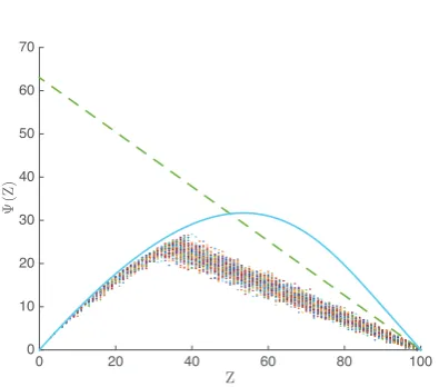
0 20 40 60 80 100
[image:9.595.72.270.70.244.2]Ψ (Z) 0 10 20 30 40 50 60 70
Fig. 3: Illustrating bounds on Ψt(Z) vs Z for N = 100
vertices and b = 1. The dashed line indicates bound (9) , the solid line bound (14) and the dots indicate values of (8) forn(i, t)drawn uniformly at random from the feasible set.
Proof: When Z =N the LHS of (12) is formally zero and the inequality holds trivially. Otherwise, we maximise over
n the concave function P
i∈N \Z
1−∆+1−b
∆+1 ni
subject
to linear constraint (11). Since we want an upper bound, we can work on the relaxed problem in which we allown∈RN,
because the maximum over this wider set will be greater than or equal to the maximum over ZN. This relaxed optimisation is convex. The Slater condition is satisfied, because ∆ > 1
andZ≥1and so the pointni= 0∀iis in the interior of the
constraint set. Hence, strong duality holds. The Lagrangian is
L=−P
i∈N \Z
1−∆+1−b
∆+1 ni
+µ(P
i∈N \Zni−∆Z)
and the main KKT conditions are−∆+1∆+1−bnilog∆+1−b
∆+1 =
µ, i ∈ N \ Z. It follows that ni = nj for all i, j ∈ N \
Z. Further, since 0 < ∆+1∆+1−b < 1 and the ni are finite
it follows that µ > 0 and so by complementary slackness constraint (11) is tight. Hence, theni maximisingf are
ni=
∆Z
N−Z, i∈ N \ Z. Z < N, (13)
Substituting intoP
i∈N \Z
1−∆+1−b
∆+1 ni
now yields the
stated result.
Using Lemma 4 it follows from (8) that,
Ψt(Z)≤ 1−
∆+1−b
∆+1 N∆−ZZ
!
(N−Z) =:ψ(Z). (14)
The boundψ(Z)depends only on the cardinalityZ of setZ and it can be verified (by inspection of the second derivative) that ψ(Z) in (14) is concave inZ as required. Observe also thatψ(Z)is time-invariant.
The upper bound (14) is considerably tighter than (9) asZ
approaches 0. This can be seen, for example, in Figure 3.
C. Some Useful Identities
The following lemma summarises identities that will prove useful in the next section.
Lemma 5. Let ∆ :=˜ ∆+1−b
∆+1 . For∆≥1we have that: (i) The range of∆˜1α−∆α is[e−1−αα,1]for any0< α <1;
(ii) ∆˜(∆+1) is increasing in∆; (iii) lim∆→∞∆˜(∆+1)= 1/eb.
(iv) ekb <1 for0< b≤1wherek= 1 + 2 log
2 2−b.
Proof: (i) The derivative of ∆˜1α−∆α with respect to ∆ is ˜
∆1α−∆α α
1−α
b
(∆+1) ∆
∆+1−b+ log ˜∆
< 0. When ∆ ≥ 1 and
α
1−α > 0, 0 < b ≤ 1 it follows that ∆˜
α∆
1−α is decreasing.
Hence, it takes its maximum value of 2−2b
α
1−α < 1
when ∆ = 1 and its minimum as ∆ → ∞ is e−b1−αα ≥ e−1−αα. (ii) The derivative of ∆˜(∆+1) with respect to ∆ is
˜
∆∆+1 b
∆+1−b+ log ˜∆
> 0 when ∆ ≥ 1. It follows that
˜
∆(∆+1) is increasing as claimed. (iii) Follows from the limit form ofe. (iv) It can be verified by inspection of the derivative that ekb is strictly decreasing on interval 0 < b ≤ 1. Hence,
k
eb < e10 = 1.
D. BoundingE[Zt]As Time Elapses
As already noted, the main challenge in the analysis is controlling the ψt(·) term in (5) as time elapses. Combining
(6) and (14) we have that
EZS
τ+1
≤∆˜EZS
τ
+
1−
˜ ∆
∆E[ZSτ]
N−E[ZSτ]
(N−E
ZSτ
), (15)
where∆ :=˜ ∆+1∆+1−b.
To proceed we would like to substitute in (15) an upper bound onE
ZSτ
rather than using the exact value. However, for the inequality in (15) to continue to hold after this substitution requires that the RHS of (15) is monotonically increasing in EZS
τ
. The first term on the RHS of (15) is linear and increasing since∆>0and1−b≥0. The following lemma establishes that the second term on the RHS of (15) is also increasing.
Lemma 6 (Increasing). Let f(Z) :=1−∆˜N∆−ZZ
(N−Z)
with ∆ :=˜ ∆+1−b
∆+1 . Then f(Z) ≤ f(Y) whenever 0 ≤
Z ≤ Y ≤ αN for any 0 ≤ α ≤ α∗ where α∗ satisfies
α∗=h(e− α
∗
1−α∗)withh(x) = xlogx
x−1 . Note thatα= 1 2 is one admissible choice.
Proof: It can be verified by inspection of the second derivative that f(Z) is concave for Z ∈ [0, N]. Hence, the supporting hyperplane property holds i. e. f(Z) ≤ f(Y)− (Y −Z)f′(Y). For Z ≤Y then when f′(Y)≥0 it follows
thatf(Z)≤f(Y)as required. By the monotonicity of the sub gradients of concave functions(f′(Y)−f′(Z))(Y −Z)≤0. Hence, for Y ≤αN then(f′(αN)−f′(Y))(αN −Y)≤0
i. e. f′(Y) ≥ f′(αN) and for f′(Y) ≥ 0 it is sufficient to show that f′(αN)≥0. Now,
f′(αN) =−1 + ˜∆1α−∆α− 1 α∆˜
α∆
(1−α)log ˜∆(1α−∆α)
The functionf˜(x) =−1 +x−1
αxlogxis concave on[0,∞)
(the second derivative is negative for all x ∈ [0,∞)), and has its global maximum (equal to −1 + 1
x∗ = eα−1 < 1. It is strictly increasing on the left side and strictly decreasing on the right side of this maximum.
˜
f(x) has one root to the right of this maximum atx+ = 1 and a second root x− to the left at the point satisfying
α= x−logx−
x−−1 . By Lemma 5,∆˜
α∆
1−α takes values in[e−1−αα,1].
Recall that x+ = 1. Observe that since h(x) = xxlog−1x is strictly increasing, so is its inverse h−1(·). Hence, for
α ≤ h(e−1−αα) then x− = h−1(α) ≤ e−1−αα. It follows
thatf˜(x)is non-negative in[e−1−αα,1]. It can be verified that h(e−1)> 1
2 and soα= 12 is an admissible choice. Observing thatf′(αN) = ˜f( ˜∆α∆
α−1)it follows thatf′(αN)≥0and we
are done.
Note that the condition in Lemma 6 is tight in the sense that for a graph with sufficiently large degree∆the functionf(·)is not increasing whenα > α∗. Lemma 6 allows us to substitute an upper bound on E
ZSτ
into (15). However, as we will shortly see, the resulting expression is still too complex to be manageable. To obtain a tractable expression we need to use the following Lemma.
Lemma 7 (Clean Upper Bound). For any ∆≥1,τ ≥1 and
0< b≤1we have
˜
∆τ(∆+1)+1kτ−1+ 1−∆˜ ∆ ˜∆
τ(∆+1)kτ−1 1−∆˜τ(∆+1)kτ−1
!
(1−∆˜τ(∆+1)kτ−1)
≤kτ∆˜τ(∆+1)+1, (16) where∆ :=˜ ∆+1∆+1−b and k= 1 + 2 log2−2b.
Proof: The required bound (16) can be rewritten equiva-lently as
1
kF(∆, Y)≤1,
with
F(∆, Y) = 1 +Y ∆ + 1 ∆ + 1−b
1−
∆ + 1
−b ∆ + 1
∆/Y
.
and Y(X) := 1−XX, X(∆, τ) := ∆+1∆+1−bτ(∆+1)kτ−1. By Lemma 5 ∆˜τ(∆+1) is increasing in ∆. It follows that
X(∆, τ) is increasing in ∆ since τ ≥ 1. Further, X(∆, τ)
is decreasing in τ since its derivative with respect to τ
is ∆˜τ(∆+1)kτ−1logk∆˜∆+1 ≤ e−bτkτ−1logk/eb ≤ 0 as
k < eb for0 < b≤ 1, τ ≥1 andlim
∆→∞∆˜(∆+1) = 1/eb
(see Lemma 5). Hence, X(∆, τ) is bounded from above by
1/eb(sinceX(∆, τ)is increasing with∆and decreasing with
τ, taking the limit as ∆→ ∞we get 1/eb when τ = 1) and
from below by 0. It follows that Y(X) ∈ [eb −1,∞). It
can be verified by inspection of the derivative that F(∆, Y)
is increasing with Y, so we can bound it from above with
F∗(∆) = lim
Y→∞F(∆, Y) = 1−log
∆+1−b
∆+1 ∆+1
. That is, 1
kF(∆, Y)≤
1
kF∗(∆). NowF∗(∆)is decreasing with∆and
sok1F(∆, Y)≤ 1
kF∗(∆)≤
1
kF∗(1) =
1+2 log 2/(2−b)
k = 1for
∆∈ {1,2, . . .} as required.
It can be seen that the expression on the LHS of (16) is quite complicated and the upper bound on the RHS in Lemma 7, which is essential for our analysis, is not obvious. It has been
obtained by considering the limiting case when∆→ ∞and building an ansatz that is exponential decaying with τ.
E. Proof of Theorem 2
Armed with Lemmas 6 and 7 we are now in a position to prove Theorem 2. For the first S1 − 1 steps, vertices in the permanent state cannot become dissatisfied, so as shown in (4) we have EZS
1
≤ φ(S1−1)(E[Z
1]). Since
φ(Z) is strictly increasing in Z we can bound E[Z1] with
N, obtaining EZS
1
≤ ∆˜S1−1N ≤ ∆˜S−1N, where S := minτ∈{1,2,··· }Sτ+1−Sτ ≥0is the minimum interval between
the Sτ’s and we have used the fact that 0 < ∆˜ < 1. When
S ≥∆ + 1 we have that∆˜S−1 ≤ 1
2 provided that b= 1. It then it follows thatE
ZS1
≤N/2 and we can use Lemma 6 to bound (15) with
E
ZS1+1
≤∆˜S+1N+
1−∆˜N∆ ˜−∆∆˜S NS N
(N−∆˜SN).
This expression is still too complicated to be used in (4) for the nextS2 slots, but whenS≥∆ + 1then we can obtain a clean upper bound using Lemma 7 withτ = 1. Namely,
EZS
1+1
≤kN∆˜(∆+1)+1
(a)
≤ k ebN,
where (a) follows from Lemma 5. For the subsequent slots
S1+ 1throughS2−1, vertices in the permanent state cannot become dissatisfied, soψt(Z) = 0and
EZS
2
≤∆˜S2−S1−1EZ
S1+1
≤∆˜2S−1EZS
1+1
≤kN∆˜2(∆+1)≤ kN
e2b.
Whenb≥ 2
3 then we have
k e2b <
1
2 and we can again apply Lemma 6 to obtain
E
Z2S+1
≤∆˜2(∆+1)+1
N+ 1−∆˜N∆ ˜−∆2(∆+1)∆2(∆+1)˜ NN
!
(N−∆˜2(∆+1)
N).
Now we can apply Lemma 7 again withτ = 2.
Iterating this procedure, for allτ = 1,2,· · · we obtain
E
ZSτ
≤kτ−1N∆˜τ(∆+1). (17) With bound (17) we are now almost done. By Lemma 5 we have∆˜(∆+1)≤e−band so the RHS of (17) is upper bounded
by Nk(k
eb)τ. Since ekb <1(by Lemma 5) then (17) establishes
thatE[Zt]is decreasing at the sequence of timest∈ S.
Recalling that P ZS
τ ≥1
≤ E
ZSτ
, to ensure
P ZS
τ ≥1
≤ ǫ it follows from (17) that it is enough to choose
τ ≥B(N,∆, ǫ), (18)
where B(N,∆, ǫ) := logN+log (ǫ−1)+log (k−1)
(∆+1) log (∆+1∆ )+log (k−1), from which
Theorem 2 now follows.
Bound (18) gives the convergence rate in terms of the reset timesSτ. When we haveSτ+1−Sτ ≤M for allt= 1,2,· · ·
Taking the limit ofMlogN+log (1+log (ǫ−1k)+log (−1) k−1) asN,∆→ ∞
now yields Corollary 2. Corollary 3 is obtained settingM = ∆+1and assuming∆≤β. Corollary 4 is obtained by setting
M = ∆ + 1and assuminglimN,∆→∞∆N =β >0.
F. Discussion
In this analysis we have taken care to ensure that the bounds used are tight i. e. there exists a graph and an assignment of colours for which they are satisfied with equality. This suggests that the bound on convergence rate in Theorem 2 is probably almost as good as we can do without restricting attention to specific types of graph.
The requirement in Theorem 2 that Sτ+1− Sτ ≥ ∆ + 1
arises from Lemma 7, until that point there is no restriction on the choice of the reset timesSτ. Extending the analysis to
settings whereSτ+1−Sτ <∆+1therefore requires extending
Lemma 7. However, obtaining Lemma 7 was already a difficult step and its extension likely requires development of a new analysis approach e. g.a new stochastic concentration bound. The requirement that b = 1 arises from application of Lemma 6, until this point there is no restriction on the value of parameter b. Lemma 6 is used to ensure that the RHS of (15) is increasing and so we can substitute an upper bound for
EZS
t
while preserving the inequality. Lemma 6 itself gives an exact condition. However, it might be possible to relax the requirement onbby allowing the RHS of (15) to decrease in a controlled way and modifying the inequality in (15) after the substitution of the bound for EZS
t
accordingly. However, this also has knock-on effects on the application of Lemma 7, so we leave it as future work. An alternative is to relax the requirement thatS≥∆+1to one thatS≥∆+nwithn >1. For example, selectingn= 2ensures∆˜S−1= ˜∆∆+1≤1/eb
which is less than 1/2 forb >log(2)≈0.69.
V. NUMERICALSIMULATIONS
A. Convergence Rate
Theorem 2 only provides an upper bound on the conver-gence rate. In Figure 4 we compare the measured converconver-gence time with this bound for a range of graph types (bipartite, complete, 12-partite) and sizes (up to N = 2000 vertices), over 10 000 runs of the algorithm. Figure 4 plots the ratio between these, which can be seen to tend towards a constant value asN increases so confirming that theO((∆ + 1) logN)
behaviour in Theorem 2 indeed broadly captures the actual scaling of convergence time with N. The ratio in Figure 4 is, however, less than one which indicates that there may be scope to further refine the prefactor in the Theorem 2 bound, at least for specific classes of graphs. We note that similar results are obtained for random graphs, although we do not include them to save space.
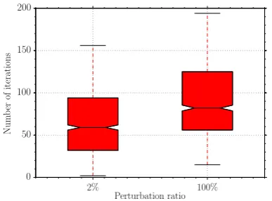
B. Behaviour on Graph Change
We analyse the case in which the algorithm has already converged to a proper coloring and then a number of vertices in the graph change change color. In Figure 5, the convergence time after a perturbation of the 2% of the vertices is shown
N
0 500 1000 1500 2000
˜R/B
(
N
,
∆
)
10-4
10-3
10-2
10-1
100
[image:11.595.330.506.91.228.2]Bipartite 12-partite Complete
Fig. 4: Ratio between measured time for simplified FCFL (Al-gorithm 2) to converge and the bound(∆ + 1)B(N,∆,1/2). Median over 10 000 runs of FCFL with parameters Sτ =
τ(∆ + 1),b= 1.
Perturbation ratio
N
um
b
er
of
it
er
at
io
ns
2% 100%
0 50 100 150 200
Fig. 5: Convergence time of FCFL for already correctly colored graph after a perturbation.
and compared to the convergence time starting from a state when all vertices are dissatisfied. The results are for complete graphs of 60 vertices with 20% of the edges removed. This is a challenging case since perturbations to the color of a vertex propagate quickly to affect many neighbours. For comparison, the corresponding measured convergence rate of the Learning-BEB algorithm (that has exponential behaviour) has also been computed. For FCFL data is shown for 1000 runs of the algorithm, but for Learning-BEB we used fewer runs as each run was extremely slow to complete being around 6 orders of magnitude longer than with FCFL even when only 2% of the nodes are perturbed, and thus are not shown in the figure. This example highlights the importance of fast convergence since with decentralised algorithms even a small perturbation can easily disrupt a strongly connected graph.
[image:11.595.328.522.310.453.2]C. Brief Application Example: Reading RFID Tags
We illustrate application of the FCFL to avoid collisions when reading RFID tags. Communication from the tags to the reader can fail when there is a collision,i. e.when at least two RFID tags within the coverage of the reader transmit at the same time. To mitigate this, the RFID protocol implements a basic slotted Aloha collision resolution mechanism [10, 19, 22].
When the reader needs to identify a tag, it issues a QUERY command, and each tag in the coverage area selects an integer u.a.r. in interval [0, D−1], where parameter D−1 is set by the reader. All tags that select 0 reply immediately; tags that select another number record those numbers in a counter and don’t transmit. A tag replies by sending a16bit random number. If the reader hears the random number, it echoes that number back as an acknowledgement, causing the tag to send its Electronic Product Code (EPC). The reader can then send commands specific to that tag, or continue to inventory other tags. In case of collision or the need for another identification, the reader can issue a QUERY REP command, causing all of the tags to decrement their counters by 1; again, any tag reaching a counter value of 0 will respond. After M steps, the procedure can start again with a QUERY command. The reader can set a flag (flag B) on successfully read tags, so they will not answer anymore to subsequent queries until the tag reverts to flag A (usually after a time between500 msand5 s, but no upper limit is set in the protocol).
Our aim is to implement a collision resolution mechanism that possesses the following properties: (i) allows tags to be detected quickly (reading time comparable with Aloha); (ii) allows subsequent reads per tag to be faster; (iii) allows the reader to correctly read all of the tags when their relative posi-tions change; (iv) the new mechanism is backward compatible
i. e.able to work with both standard RFID tags and new tags. The task of assigning a different time slot (different counter value when the QUERY command is issued) to each RFID tag can be mapped to a CP on a graph, where the structure of the graph depends on the location of the tags. Namely, graph
G= (N,E)is built such thatN is the set of tags, and an edge
e= (i, j)∈ E iff the tags iand j are near enough for their transmissions to potentially collide. When all tags are within the coverage range of the reader, the problem is mapped to colouring of a complete graph. More generally (e. g. when the reader can cover at most k tags per time), many RFID applications can be modeled as a CP on a complete k-partite graphGs1,...,sk,i. e.the graph composed ofkindependent sets
of (possibly different) sizesi, i= 1, . . . , k, such that each set
is connected with all the vertices of the other sets. This graph isk-colourable.
The FCFL algorithm can be implemented in an existing RFID infrastructure, ensuring backward compatibility, as fol-lows. The idea is to modify the behaviour of the tag to allow it to enter the permanent state after a successful QUERY, and to possibly exit it every S periods by extending the meaning of the QueryAdjustcommand. The QueryAdjust command is normally used to modify the range [0, D−1] in the tags, to reduce the collision probability when many tags are present,
or to reduce the expected backoff when few of them are present. A way to implement the reset capability is to let the tag exit the permanent state when a QueryAdjust command is received3. Modified tags will thus have the following additional capabilities: (i) if the reader sets flag B the tag will enter thepermanentstate, keeping in memory the random number that allowed the communication, and stop answering to queries, (ii) if the tag receives a QueryAdjust broadcast command it will exit the permanent state by reverting to flag A and thus becoming ready to decrement the counter when the QUERY REP command is broadcast again. As for the QUERY command, if the stored counter is equal to 0, the tag will immediately attempt transmission. The reader is programmed to send a QueryAdjust command every S period, i. e. every
S·Dqueries, immediately after the QUERY command, so that the tags that are leaving the permanent state will still select the same random number, to potentially re-enter immediately the permanent state, if no tag is colliding with them. The reader also sets flag B on each tag that is correctly detected in a time slot not used by previously detected tags. In this way already identified tags will not cause collisions, and tags that are correctly identified but that would cause a collision (with a previous identified tag) will continue to change.
This implementation will still work together with non-modified tags at the expense of having some collisions, be-cause those non-modified tags will choose a new (possibly different) time slot at every new QUERY, but each non modified tag can at most affect one modified tag, so the overall performance should still be superior to the standard slotted Aloha mechanism.
We compare the convergence time of the FCFL algorithm to each of the following algorithms from [16]:
BFSA Basic Framed Slotted Aloha, with standard superframe size ofD= 256slots.
DFSA Dynamic Framed Slotted Aloha, where the superframe sizeDdoubles when the number of slots with collisions is larger than 70 % of the current superframe size, and halves when the number of slots with collisions is less than30 %.
EDFSA Enhanced Dynamic Framed Slotted Aloha, see [16] for more details of this enhanced version of DFSA. For these algorithms the superframe size D is the number of slots after which the reader starts a new QUERY (forcing the tags to select a new slot u.a.r.). These algorithms are all
memorylessin the sense that over each superframe they behave statistically in the same way. In contrast, the FCFL algorithm has a transient period during which a collision-free schedule is determined and after which tags will deterministically select the same slot at every subsequent superframe in a collision-free manner.
Measurements of time taken to read all tags are given in Table I for these algorithms. It can be seen that the FCFL algorithm is comparable with classic slotted Aloha during the transient period, but once in steady state performs considerably better (yielding a83 %reduction in read time), and also better
Algorithm 3 Simplified Fast Communication-Free Learning for RFID
Reader block
1: Broadcast QueryAdjust command withD ⊲Reset 2: Initialise countert= 0
3: repeat
4: ift= 0 modDthen
5: Broadcast QUERY command 6: ift= 0 modSD then
7: Broadcast QueryAdjust command withD
8: end if
9: else
10: Broadcast QUERY REP command
11: ifNew tagT detected in an unused slotthen
12: Add T to inventory ⊲ (and any additional operation)
13: Set Flag=B to tagT
14: end if
15: end if
16: t=t+1 17: untilForever
Tag block
18: ifFlag=Athen19: ifC= 0then
20: Send EPC to reader and establish connection
21: end if
22: ifReceived QUERY commandthen
23: Select an integerC in[0, D−1]
24: end if
25: ifReceived QUERY REPthen
26: C=C−1
27: end if
28: else ⊲Flag=B
29: ifReceived QueryAdjustthen
30: Set Flag=A,C=C−1
31: end if
32: end if
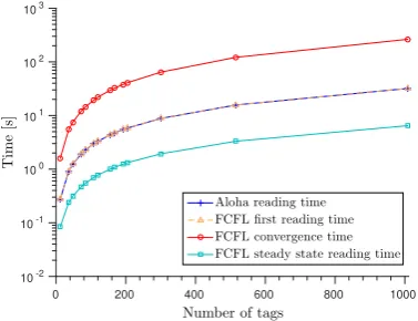
than the state-of-the-art dynamically adjusted slotted Aloha (over which FCFL offers a66 %reduction in read time). Using the ISO15693 high tag data rate [22], the reader needs at each slot 1 ms to send the QUERY (or QUERY REP) command, and the tag needs6 msto complete the identification procedure with the reader (for transmission of the random number and reception of the echo acknowledgement). This would mean that FCFL allows 1000 tags to be read in around 7 seconds compared with more than40seconds for classic slotted Aloha.
Figure 6 plots the measured convergence time (median over
10 000 runs), the time taken to read all tags initially and the time taken in steady state. Data is shown both for FCFL and classic slotted Aloha with flagging enabled and superframe sizeDequal to∆ + 1. It can be seen that the initial read time is comparable for the both algorithms, but after convergence (less than 5 minutes for a shelf of 1000 items) the FCFL algorithm is able to check the status of all tags within 7
seconds, compared with the 32 seconds required by Aloha,
200 tags 1000 tags
Algorithm First inventory At steady state First inventory At steady state
BFSA 1280 1280 5850 5850
DFSA 662 662 5425 5425
EDFSA 628 628 2916 2916
[image:13.595.47.291.112.513.2]FCFL 816 200 5040 1000
TABLE I: Median number of time slots needed to correctly read all tags vs the algorithm used (for FCFL we used the simplified version, i. e. Algorithm 2). Complete graph with
N= 200 andN= 1000.
Number of tags
0 200 400 600 800 1000
T
im
e
[s
]
10-2 10-1 100 101 102 103
Aloha reading time FCFLfirst reading time FCFL convergence time FCFL steady state reading time
Fig. 6: Reading time of simplified FCFL (Algorithm 2) and slotted Aloha vs number of tags. 12-partite complete graph. Median over10 000runs.
a time saving of around450%.
VI. CONCLUSIONS ANDFUTUREWORK
In this paper we consider algorithms for quickly solving, in a fully decentralised way (i. e. with no message passing), the classic problem of colouring a graph. We propose a novel algorithm that is automatically responsive to topology changes, and we prove that it converges quickly to a proper colouring in O(NlogN)time with high probability for generic graphs (and in O(logN) time if ∆ = O(1)) when the number of available colours is greater than ∆, the maximum degree of the graph. We believe the proof techniques used in this work are of independent interest and provide new insight into the properties required to ensure fast convergence of decentralised algorithms.
We note that application of FCFL to general constraint satisfaction problems is direct, but we leave analysis of con-vergence rate in this more general setting to future work.
ACKNOWLEDGMENTS
We want to thank Jaume Barcelo, Joan Meli-Segu and Marc Morenza for their thoughtful insights. Their expertise on RFID and Learning-BEB substantially improved this work.
REFERENCES
[image:13.595.328.517.210.355.2]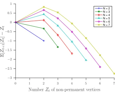
![Fig. 2: Illustrating evolution of E[Zt|Z1] vs time t. At timest ∈ S the drift may be positive and the value may increasecompared to time t − 1 ∈ S¯](https://thumb-us.123doks.com/thumbv2/123dok_us/7738437.164448/6.595.79.262.83.227/illustrating-evolution-timest-drift-positive-value-increasecompared-time.webp)