Preconditioned ADMM with nonlinear operator constraint

operator constraint

Martin Benning1_{, Florian Knoll}2_{, Carola-Bibiane Sch¨onlieb}1_{, and} Tuomo Valkonen1

1

University of Cambridge, Department of Applied Mathematics and Theoretical Physics, Wilberforce Road, Cambridge CB3 0WA, United Kingdom

({mb941, cbs31, tjmv3}@cam.ac.uk)

2

New York University, Center for Advanced Imaging, Innovation and Research, New York 4th Floor 660 First Avenue New York, NY 10016, USA

([email protected])

Abstract. We are presenting a modification of the well-known Alternat-ing Direction Method of Multipliers (ADMM) algorithm with additional preconditioning that aims at solving convex optimisation problems with nonlinear operator constraints. Connections to the recently developed Nonlinear Primal-Dual Hybrid Gradient Method (NL-PDHGM) are pre-sented, and the algorithm is demonstrated to handle the nonlinear inverse problem of parallel Magnetic Resonance Imaging (MRI).

Keywords: ADMM, primal-dual, nonlinear inverse problems, parallel MRI, proximal point method, operator splitting, iterative Bregman method

1

Introduction

Non-smooth regularisation methods are popular tools in image processing. They allow to promote sparsity of inverse problem solutions with respect to specific representations; they allow to implicitly restrict the null-space of the forward op-erator while guaranteeing noise suppression at the same time. The most promi-nent representatives of this class are total variation regularisation [20] and `1 -norm regularisation as in the broader context of compressed sensing [11,8].

In order to solve convex, non-smooth regularisation methods with linear op-erator constraints computationally, first-order opop-erator splitting methods have gained increasing interest over the last decade, see [12,13,3,10] to name just a few. Despite some recent extensions to certain types of non-convex problems [17,15,7,16] there has to our knowledge only been made little progress for non-linear operators constraints [2,23].

In this paper we are particularly interested in minimising non-smooth, con-vex functionals with nonlinear operator constraints. This model covers many interesting applications; one particular application that we are going to address is the joint reconstruction of the spin-proton-density and coil sensitivity maps in parallel MRI [22,14].

The paper is structured as follows: we will introduce the generic problem formulation, then address its numerical minimisation via a generalised ADMM method with linearised operator constraints. Subsequently we will show connec-tions to the recently proposed NL-PDHGM method (indicating a local conver-gence result of the proposed algorithm) and conclude with the joint spin-proton-density and coil sensitivity map estimation as a numerical example.

2

Problem formulation

We consider the following generic constrained minimisation problem:

(ˆu,v) = arg minˆ u,v

{H(u) +J(v) subject toF(u, v) =c} . (1)

Here H andJ denote proper, convex and lower semi-continuous functionals,F is a nonlinear operator andca given function. Note that for nonlinear operators of the formF(u, v) =G(u)−vandc= 0 problem (1) can be written as

ˆ

u= arg min u

{H(u) +J(G(u))}. (2)

In the following we want to propose a strategy for solving (1) that is based on simultaneous linearisation of the nonlinear operator constraint and the solution of an inexact ADMM problem.

3

Alternating direction method of multipliers

We solve (1) by alternating optimisation of the augmented Lagrange function

Lδ(u, v;µ) =H(u) +J(v) +hµ, F(u, v)−ci+ δ

2kF(u, v)−ck 2

2. (3)

Alternating minimisation of (3) inu,v and subsequent maximisation ofµvia a step of gradient ascent yields this nonlinear version of ADMM [12]:

uk+1∈arg min u

_δ

2kF(u, v

k_)−ck2 2+hµ

k_{, F(u, v}k_)i+H(u)

, (4)

vk+1∈arg min v

_δ

2kF(u

k+1_{, v)−ck}2 2+hµ

k_{, F(u}k+1_{, v)i+J(v)}

, (5)

µk+1=µk+δ F(uk+1, vk+1)−c. (6)

Not having to deal with nonlinear subproblems, we replace F(uk+1_{, v}k_{) and} F(uk+1_{, v}k+1_{) by their Taylor linearisations around u}k _{and v}k_{, which yields} F(u, vk_{) ≈ F(u}k_{, v}k_{) +∂uF(u}k_{, v}k_{) u−u}k

and F(uk+1_{, v) ≈ F(u}k+1_{, v}k_{) +} ∂vF(uk+1, vk) v−vk

, respectively. The updates (4) and (5) modify to

uk+1∈arg min u _δ 2 A k_u −ck₁

2 2+hµ

k_{, A}k_u

i+H(u)

, (7)

vk+1∈arg min v

_δ

2

Bkv−ck₂

2 2+hµ

k_{, B}k_vi+J(v)

with Ak _:=∂uF(uk_{, v}k_),Bk _:=∂vF(uk+1_{, v}k_{), c}k

1 :=c+Akuk−F(uk, vk) and ck₂:=c+Bkvk−F(uk+1, vk). Note that the updates (7) and (8) are still implicit, regardless of H and J. In the following, we want to modify the updates such that they become simple proximity operations.

4

Preconditioned ADMM

Based on [24], we modify (7) and (8) by adding the surrogate terms kuk+1₋ uk_k2

Qk

1

/2 andkvk+1_−vk_k2 Qk

2

/2, withkwkQ:=

p

hQw, wi(note that ifQis chosen to be positive definite,k · kQ becomes a norm). We then obtain

uk+1∈arg min u _δ 2 A k u−ck1

2 2+hµ

k

, Akui+H(u) +1 2ku−u

k k2_Qk

1

,

vk+1∈arg min v

_δ

2

Bkv−ck₂

2 2+hµ

k_{, B}k_v

i+J(v) +1 2kv−v

k k2_Qk

2

.

If we chooseQk

1 :=τ1kI−δAk∗Ak withτ1kδ <1/kAkk2andQk2:=τ2kI−δBk∗Bk withτk

2δ <1/kBkk2 and if we defineµk:= 2µk−µk−1 we obtain

uk+1= I+τ₁k∂H−1

uk−τ₁kAk∗µk

, (9)

vk+1= I+τ₂k∂J−1

vk−τ₂kBk∗ µk+δ F(uk+1, vk)−c

, (10)

with (I+α∂E)−1(w) denoting the proximity or resolvent operator

(I+α∂E)−1(w) := arg min u

₁

2ku−wk 2

2+αE(u)

.

The entire proposed algorithm with updates (9), (10) and (6) reads as

Algorithm 1Preconditioned ADMM with nonlinear operator constraint

Parameters:H, J, F, c

Initialization:u0,v0,µ0,δ µ0_=µ0

whileconvergence criterion is not metdo

Ak_=∂

uF(uk, vk)

Setτ1k such thatτ1kδ <1/kAkk2 uk+1= I+τ1k∂H

−1

uk−τ1kAk∗µk

Bk=∂vF(uk+1, vk)

Setτk

2 such thatτ2kδ <1/kBkk2 vk+1_{= I+τ}k

2∂J −1

vk_−τk

2Bk

∗

µk_{+δ F(u}k+1_{, v}k_)−c µk+1_=µk_{+δ F(u}k+1_{, v}k+1_)−c

µk+1_{= 2µ}k+1_−µk end while

5

Connection to NL-PDHGM

In the following we want to show how the algorithm simplifies in case the non-linear operator constraint is only nonnon-linear in one variable, which is sufficient for problems of the form (2). Without loss of generality we consider constraints of the form F(u, v) = G(u)−v, whereGrepresents a nonlinear operator in u. Then we haveAk _=JG(uk_{) (withJG(u}k_{) denoting the Jacobi matrix ofGat} uk_),Bk _{=−I and if we further chooseτ}k

2 = 1/δ for allk, update (10) reads

vk+1=

I+1 δ∂J

−1

G(uk+1) +1 δµ

k

.

Applying Moreau’s identity [19]b= I+1_δ∂J−1(b) +1_δ(I+δ∂J∗)−1(δb) yields

µk+1= (I+δ∂J∗)−1 µk+δG(uk+1)

.

If we further change the order of the updates, starting with the update for µ, the whole algorithm reads

µk+1= (I+δ∂J∗)−1 µk+δG(uk)

,

µk+1= 2µk+1−µk,

uk+1= I+τ1k∂H

−1

uk−τ1kJG(uk)∗µk+1

.

Note that this algorithm is almost the same as NL-PDHGM proposed in [23] for θ = 1, except that the extrapolation step is carried out on the dual variableµ instead of the primal variableu. In the following we want to briefly sketch how to prove convergence for this algorithm in analogy to [23]. We define

N(µk+1, uk+1) :=

∂J∗(µk+1_{)− ∇G(u}k_)uk+1_−ck ∂H(uk+1_{) +JG(u}k₎∗_µk+1

,

Lk:= 1

δI JG(u k₎

JG(uk₎∗ 1 τk

1

I

!

,

withck_:=G(uk_{)− JG(u}k_)uk_{. Now the algorithm is: find (µ}k+1_{, u}k+1_{) such that} N(µk+1, uk+1) +Lk(µk+1−µk, uk+1−uk)30.

If we exchange the order of µand uhere, i.e., reorder the rows of N, and the rows and columns ofLk_{, we obtainalmost the “linearised” NL-PDHGM of [23].} The difference is that the sign of JG in Lk _{is inverted. The only points in} [23] where the exact structure of Lk _(M

xk therein) is used, are Lemma 3.1,

6

Joint estimation of the spin-proton density and coil

sensitivities in parallel MRI

We want to demonstrate the numerical capabilities of the algorithm by applying it to the nonlinear problem of joint estimation of the spin-proton density and the coil sensitivities in parallel MRI. The discrete problem of joint reconstruction from sub-sampled k-space data on a rectangular grid reads

     ˆ u ˆ c1 .. . ˆ c2     

∈ arg min v=(u,c1,...,cn)

   1 2 n X j=1

kSF(G(v))j−fjk22+α0R0(u) + n

X

j=1

αjRj(cj)

  

,

whereF is the 2D discrete Fourier transform,fj are the k-space measurements for each of thencoils,Sis the sub-sampling operator andRjdenote appropriate regularisation functionals. The nonlinear operator G maps the unknown spin-proton densityuand the different coil sensitivitiescj as follows [22]:

G(u, c1, . . . , cn) = (uc1, uc2, . . . , ucn)T. (11)

In order to compensate for sub-sampling artefacts in sub-sampled MRI it is com-mon practice to use total variation as a regulariser [6,18]. Coil sensitivities are assumed to be smooth, cf. Figure 6, motivating a reconstruction model simi-lar to the one proposed in [14]. We therefore choose the discrete isotropic total variation,R0(u) =k∇uk2,1, and the smooth 2-norm of the discretised gradient, i.e. Rj(cj) := k∇cjk2,2, for all j > 0, following the notation in [4]. We further introduce regularisation parametersλj in front of the data fidelities and rescale all regularisation parameters such thatα0+Pn_j=1λj+Pn_j=1αj= 1. In order to realise this model via Algorithm 1 we consider the following operator splitting strategy. We defineF(u0, . . . , un, v0, . . . , v2n) as

F(u0, . . . , un, v1, . . . , vn) :=

       

G(u0, . . . , un) ∇u0 0 · · · 0

0 ∇u1 . .. ... ..

. . .. . .. 0 0 · · · 0 ∇un

        −         v0 .. . vn .. . v2n

        ,

setH(u0, . . . , un)≡0, andJ(v0, . . . , v2n) =P 2n

j=0Jj(vj) withJj(vj) := λj

2kSFvj− fjk2

operations can be carried out easily. In particular, we obtain

(I+τ₁k∂H)−1(w) =w,

(I+τ2k∂Jj)−1(w) =F−1

Fwj+τ2kλjSTfj 1 +τk

2λjdiag(STS)

forj∈ {0, . . . , n−1},

(I+τ₂k∂Jn)−1(w) = wn kwnk2

max kwnk2−α0τ2k,0

,

(I+τ2k∂Jj)−1(w) = wn kwnk2,2

max kwnk2,2−αjτ2k,0

forj∈ {n+ 1, . . . ,2n}.

Moreover, as Bk =−I (and thus,kBk_{k= 1) for allk, we can simply eliminate} τk

2 by replacing it with 1/δ, similar to Section 5.

6.1 Experimental setup

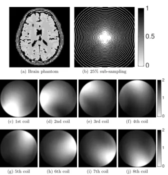
We now want to discuss the experimental setup. We want to reconstruct the synthetic brain phantom in Figure 1(a) from sub-sampled k-space measurements. The numerical phantom is based on the design in [1] with a matrix size of 190×190. It consists of several different tissue types like cerebrospinal fluid (CSF), gray matter (GM), white matter (WM) and cortical bone. Each pixel is assigned a set of MR tissue properties: Relaxation times T1(x, y) and T2(x, y) and spin density ρ(x, y). These parameters were also selected according to [1]. The MR signal s(x, y) in each pixel was then calculated by using the signal equation of a fluid attenuation inversion recovery (FLAIR) sequence [5]:

s(x, y) =ρ(x, y)(1−2 e−TI/T1(x,y)_)(1−e−TR/T1(x,y)_)e−TE/T2(x,y)_.

The sequence parameters were selected: TR = 10000 ms, TE = 90 ms. TI was set to 1781 ms to achieve signal nulling of CSF (Tcsf1 log(2) with T

csf

1 = 2569ms). In order to generate artificial k-space measurements for each coil, we proceed as follows. First, we produce 8 images of the brain phantom multiplied by the measured coil sensitivity maps shown in Figure 1(c) - 1(j). The coil sensitivity maps were generated from the measurements of a water bottle with an 8-channel head coil array. Then we produce artificial k-space data by applying the 2D discrete Fourier-transform to each of those individual images. Subsequently, we sub-sample only approx. 25% of each of the k-space datasets via the spiral shown in Figure 1(b). Finally, we add Gaußian noise with standard deviation σto the sub-sampled data.

6.2 Computations

For the actual computations we use two noisy versions fj of the simulated k-space data; one with small noise (σ= 0.05) and one with a high amount of noise (σ= 0.95). As stopping criterion we simply choose a fixed number of iterations; for both the low noise level as well as the high noise level dataset we have fixed the number of iterations to 1500. The initial values used for the algorithm are u0_j =1with1∈Rl×1 being the constant one-vector, for all j∈ {0, . . . , n}. All

(a) Brain phantom (b) 25% sub-sampling

1

0.5

0

(c) 1st coil (d) 2nd coil (e) 3rd coil (f) 4th coil

2

1

0

(g) 5th coil (h) 6th coil (i) 7th coil (j) 8th coil

2

1

0

Fig. 1.Figure 1(a) shows the brain phantom as described in Section 6.1. Figure 1(c) - 1(j) show visualisations of the measured coil sensitivities of a water bottle. Figure 1(b) shows the simulated, spiral-shaped sub-sampling scheme used to sub-sample the k-space data.

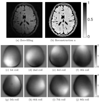
(a) Zero-filling (b) Reconstructionu

1

0.5

0

(c) 1st coil (d) 2nd coil (e) 3rd coil (f) 4th coil

2

1

0

(g) 5th coil (h) 6th coil (i) 7th coil (j) 8th coil

2

1

0

Fig. 2. Reconstructions for noise with low noise level σ = 0.05. Despite the sub-sampling, features of the brain phantom are very well preserved. In addition, the coil sensitivities seem to correspond well to the original ones, despite a slight loss of con-trast. Note that coil sensitivities remain the initial value where the signal is zero.

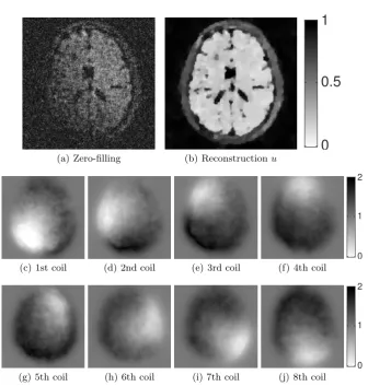
High noise level We proceeded as in the previous section, but for noisy data with noise levelσ= 0.95. The regularisation parameters were set toλj= 0.0149, α0 = 0.0135 and αj = 0.9716 for j ∈ {1, . . . , n}. The modulus images of the results are visualised in Figure 6.1. The PSNR values for the averaged zero-filled reconstruction is 9.9621, whereas the PSNR of the reconstruction with the proposed method is 16.672.

7

Conclusions & outlook

(a) Zero-filling (b) Reconstructionu

1

0.5

0

(c) 1st coil (d) 2nd coil (e) 3rd coil (f) 4th coil

2

1

0

(g) 5th coil (h) 6th coil (i) 7th coil (j) 8th coil

2

1

0

Fig. 3. Reconstructions for noise with high noise level σ = 0.95. Due to the large amount of noise, higher regularisation parameters are necessary. As a consequence, fine structures are smoothed out and in contrast to the case of little noise, compensation of sub-sampling artefacts is less successful.

the connection to the recently proposed NL-PDHGM algorithm which implies local convergence results in analogy to those derived in [23]. Subsequently we have demonstrated the computational capabilities of the algorithm by applying it to a nonlinear joint reconstruction problem in parallel MRI.

synthetic and real data would also be desirable. Moreover, future research focus will be on alternative regularisation functions, e.g. based on spherical harmonics motivated by [21]. Last but not least, other applications that can be modelled via (1) should be considered in future research.

Acknowledgments MB, CS and TV acknowledge EPSRC grant EP/M00483X/1. FK ackowledges National Institutes of Health grant NIH P41 EB017183.

References

1. Berengere Aubert-Broche, Alan C Evans, and Louis Collins. A new improved version of the realistic digital brain phantom. NeuroImage, 32(1):138–145, 2006. 2. Markus Bachmayr and Martin Burger. Iterative total variation schemes for

non-linear inverse problems. Inverse Problems, 25(10):105004, 2009.

3. Amir Beck and Marc Teboulle. Fast gradient-based algorithms for constrained total variation image denoising and deblurring problems. Image Processing, IEEE Transactions on, 18(11):2419–2434, 2009.

4. Martin Benning, Lynn Gladden, Daniel Holland, Carola-Bibiane Sch¨onlieb, and Tuomo Valkonen. Phase reconstruction from velocity-encoded mri measurements– a survey of sparsity-promoting variational approaches. Journal of Magnetic Reso-nance, 238:26–43, 2014.

5. Matt A Bernstein, Kevin F King, and Xiaohong Joe Zhou.Handbook of MRI pulse sequences. Elsevier, 2004.

6. Kai Tobias Block, Martin Uecker, and Jens Frahm. Undersampled radial mri with multiple coils. iterative image reconstruction using a total variation constraint.

Magnetic resonance in medicine, 57(6):1086–1098, 2007.

7. S. Bonettini, I. Loris, F. Porta, and M. Prato. Variable metric inexact line-search based methods for nonsmooth optimization. Siam Journal on Optimization, 2015. Submitted.

8. Emmanuel J Candes et al. Compressive sampling. In Proceedings of the inter-national congress of mathematicians, volume 3, pages 1433–1452. Madrid, Spain, 2006.

9. Antonin Chambolle. An algorithm for total variation minimization and applica-tions. Journal of Mathematical imaging and vision, 20(1-2):89–97, 2004.

10. Antonin Chambolle and Thomas Pock. A first-order primal-dual algorithm for convex problems with applications to imaging. Journal of Mathematical Imaging and Vision, 40(1):120–145, 2011.

11. David L Donoho. Compressed sensing. Information Theory, IEEE Transactions on, 52(4):1289–1306, 2006.

12. Daniel Gabay. Applications of the method of multipliers to variational inequalities.

Studies in mathematics and its applications, 15:299–331, 1983.

13. Tom Goldstein and Stanley Osher. The split bregman method for l1-regularized problems. SIAM Journal on Imaging Sciences, 2(2):323–343, 2009.

14. Florian Knoll, Christian Clason, Kristian Bredies, Martin Uecker, and Rudolf Stoll-berger. Parallel imaging with nonlinear reconstruction using variational penalties.

Magnetic Resonance in Medicine, 67(1):34–41, 2012.

16. M. M¨oller, M. Benning, C. Sch¨onlieb, and D. Cremers. Variational depth from focus reconstruction. Image Processing, IEEE Transactions on, 24(12):5369–5378, Dec 2015.

17. Peter Ochs, Yunjin Chen, Thomas Brox, and Thomas Pock. ipiano: inertial prox-imal algorithm for nonconvex optimization. SIAM Journal on Imaging Sciences, 7(2):1388–1419, 2014.

18. Sathish Ramani, Jeffrey Fessler, et al. Parallel mr image reconstruction using aug-mented lagrangian methods. Medical imaging, IEEE Transactions on, 30(3):694– 706, 2011.

19. R Tyrrell Rockafellar. Convex analysis (princeton mathematical series).Princeton University Press, 46:49, 1970.

20. Leonid I Rudin, Stanley Osher, and Emad Fatemi. Nonlinear total variation based noise removal algorithms. Physica D: Nonlinear Phenomena, 60(1):259–268, 1992. 21. Alessandro Sbrizzi, Hans Hoogduin, Jan J Lagendijk, Peter Luijten, and Cor-nelis AT den Berg. Robust reconstruction of b1+ maps by projection into a spherical functions space. Magnetic Resonance in Medicine, 71(1):394–401, 2014. 22. Martin Uecker, Thorsten Hohage, Kai Tobias Block, and Jens Frahm. Image

re-construction by regularized nonlinear inversionjoint estimation of coil sensitivities and image content. Magnetic Resonance in Medicine, 60(3):674–682, 2008. 23. Tuomo Valkonen. A primal–dual hybrid gradient method for nonlinear operators

with applications to mri. Inverse Problems, 30(5):055012, 2014.