Small Area Estimation with Skewed Data

S

MALL

A

REA

E

STIMATION WITH

S

KEWED

D

ATA

H

UKUM

C

HANDRA

,

R

AY

C

HAMBERS

A

BSTRACT

In business surveys, data typically are skewed and the standard approach for small area estimation based on linear mixed models lead to inefficient estimates. In this paper, we discuss small area estimation techniques for skewed data that are linear following a suitable transformation. In this context, implementation of the empirical best linear unbiased prediction (EBLUP) approach under transformation to a linear mixed model is complicated. However, this is not the case with the model-based direct (MBD) approach (Chambers and Chandra, 2006), which is based on weighted linear estimators. We extend the MBD approach to skewed data using sample weights derived via model calibration based on a log transform model with random area effects. Our results show this estimator is both efficient and robust with respect to the distribution of these random effects. An application to real data demonstrates the satisfactory performance of the method.

Small Area Estimation with Skewed Data

Hukum Chandra1 and Ray Chambers 2

1. Southampton Statistical Sciences Research Institute

University of Southampton, Southampton, SO17 1BJ, UK

Email: [email protected]

2. Centre for Statistical and Survey Methodology

University of Wollongong, Wollongong, NSW, 2522, Australia

Email: [email protected]

Abstract

In business surveys, data typically are skewed and the standard approach for small area estimation based on linear mixed models lead to inefficient estimates. In this paper, we discuss small area estimation techniques for skewed data that are linear following a suitable transformation. In this context, implementation of the empirical best linear unbiased prediction (EBLUP) approach under transformation to a linear mixed model is complicated. However, this is not the case with the model-based direct (MBD) approach (Chambers and Chandra, 2006), which is based on weighted linear estimators. We extend the MBD approach to skewed data using sample weights derived via model calibration based on a log transform model with random area effects. Our results show this estimator is both efficient and robust with respect to the distribution of these random effects. An application to real data demonstrates the satisfactory performance of the method.

Key Words: Small areas, Skewed data, Model Calibration, Expected value model, Calibrated

1. Introduction

Small area estimation (SAE) is typically an increasingly important secondary objective of many sample surveys, and several methods exist in the literature (Rao, 2003). However, research is continuing on several important practical problems related to small area estimation. Standard methods for SAE such as the empirical best linear unbiased prediction (EBLUP) approach (Prasad and Rao, 1990) and the model-based direct (MBD) approach (Chambers and Chandra, 2006) assume a linear mixed model can be used to characterize the small areas of interest. However, it happens (typically for skewed data) that the variable of interest Y is linear on some transformed scale (e.g. in business surveys, often variables are linear on logarithmic scale). In this context, estimation based on linear model for Y leads to inefficient estimates. In such situation, an appropriate technique for SAE should essentially be based on a linear mixed model for a transformed variable. The use of transform variables for survey estimation with skewed data has been investigated by Carroll and Ruppert (1988), Chen and Chen (1996), Karlberg (2000) and Chambers and Dorfman (2003). In this paper we explore transform variable based estimation in context of SAE for skewed data, focussing on the widely used logarithmic (log) transformation function. Implementation of the EBLUP approach under transformation to a linear mixed model is quite complicated. However, this is not the case with the MBD approach, which is based on weighted linear estimators. In this paper we extend the MBD approach of Chambers and Chandra (2006) to small area estimation for skewed data. In particular, we consider the use of sample weights derived via model calibration (Wu and Sitter, 2001) based on a log transform model with random area effects. A simple MSE estimator for weighted small area estimation is also developed. We also relax the usual normality assumption for random errors in order to examine robustness with respect to this assumption.

2. Model Calibration for Population Estimation

In this section we briefly review model calibration for estimation of population level quantities. To start, we fix our notation. Let Y denote an N-vector of population values of a characteristic of interest, and suppose that our primary aim is estimation of the total of the values in Y (or their mean

T_y

Y ). In order to assist us in this objective, we shall assume that we have ‘access’ to X, an N×p matrix of values of p auxiliary variables that are related, in some sense, to the values in Y. In particular, we assume that the individual sample values in X are known. The non-sample values in X may not be individually known, but are assumed known at some aggregate level. At a minimum, we know the population totals T of the columns of

X. Given this set up, Deville and Särndal (1992) introduce the notation of a calibration estimator of population total of Y as

x

, ˆ

y c _{j s} j j

T =

∑

_∈ w y , where the calibration weights w_j’s are chosen to minimise their average distance (Φ_s, say) from the basic design weights, d_j =π−_j1 with , that are used in Horvitz-Thompson (HT) estimator , subject to the calibration constraint

Pr( )

j

π = j s∈ ˆ_,

y HT _{j s} j j T =

∑

_∈ d y

=

j j j

E y x_ξ h x

1 N

j j j x j s∈ w x = j= x T

∑

∑

(1)

Deville and Särndal (1992) argue “weights that perform well for the auxiliary variables also should perform well for the study variable”. However, there is an implicit underlying assumption that Y and X are linearly related that makes this a valid argument, i.e. the conventional calibration approach (Deville and Särndal, 1992, Chambers, 1997) implicitly relies on the assumption that the survey variable and the auxiliary variables are linearly related. Thus, if the underlying model is non-linear then the calibrated estimator derived under a linearity assumption cannot be very efficient. Let us assume the relationship between

Y and X can be described by a super population model

( | )= ( ; )η 2

( _j|x_j)

ξ

, V y =σ ω_j; j=1,...,N, (2) where η, typically vector-valued, and σ2 are model parameters, and the mean function

( ; )_j

h x η is a known function of x_j and η, the variance function ω_j is a known function of x_j and ( ; )h x_j η . Here and denotes the expectation and variance with respect to super population model. In matrix notation we write (2) as

ξ

E V_ξ

( | ) ( ; )

E Y X_ξ =h X η and V Y X_ξ( | )= Ω (3)

as special cases. In this context, Wu and Sitter, (2001) proposed the use of sample weights derived via model calibration. They defined the calibration estimator for population mean of Y as ˆ_c 1

j s

Y N− w y

∈

=

∑

_{j j} with weights sought to minimize the distance measure Φ_s under the constraints:

j j s∈ w =N

∑

and

∑

_{j s∈} w h x_j ( ; )_j ηˆ =

∑

N_j=1h x( ; )_j ηˆ (4) where ηˆ is a design consistent estimator for η. That is calibration is performed with respect to the population mean of the ‘fitted values’ ˆh_j =h x( ; )_j ηˆ of h x( ; )_j ηˆ . Provided the model (3) is a reasonable one, y_j is then (at least approximately) a linear function of its ‘fitted values’

ˆ ( ; )_j

h x η under this model. The basic idea of this approach is then we can carry out linear estimation using these ‘fitted or expected values’ as auxiliary variables.

The above discussion represents what might be referred to the design-based interpretation of model calibration. A model-based perspective on model calibration can be described as follows. We assume that Y and ( ; )h X η are related by the linear model of the form

01N 1 ( ; )

Y =α +α h X η ε α+ = J+ε (5)

where J denotes the ‘design matrix’ for the linear model (5) linking Y and h X( ; )η , 0 1

( , )

α = α α ′ is a vector of unknown parameters, ε denotes a N-vector of random variables with E_ξ( )ε =0 and V_ξ( )ε = Ω =[ω_jk]. We called model (5) the ‘expected value’ or ‘fitted value’ model defined by (3). For α0 =0 in model (5) we refer as ratio specification of this model, otherwise regression specification. The model (5) can have either ratio or regression specification. Without loss of generality, we arrange the vector Y so that the first n elements correspond to the sample units, and partition Y, J and Ω according to sample and non-sample units:

s r

Y Y

Y

⎡ ⎤

= ⎢ ⎥_{⎣ ⎦}, s

r

J J

J

⎡ ⎤

= ⎢ ⎥_{⎣ ⎦} and ss sr

rs rr Ω Ω

⎡ ⎤

Ω = ⎢_{⎣Ω Ω ⎦}⎥.

Here J_s is the n ×1 vector of ‘fitted values’ of the auxiliary variables and Ω_ss is the n × n covariance matrix associated with the n sample units that make up the n×1 sample vector Y_s. A subscript of r is used to denote corresponding quantities defined by the N −n non-sample units, with Ω_rs denoting the (N−n)×n matrix defined by . In what follows we denote 1 , 1 and 1 as vectors of 1’s and , and as identity matrices of order N, n and

) , (Y_r Y_s

Cov

N n r IN In Ir

unknown and so need to be estimated from the sample data. We use a “hat” to denote such an estimate. Further, throughout this paper we assume that sampling is uninformative, so the sample data also follow the population model.

Given this notation, the sample weights that define the BLUP for population total of Y under a general linear ‘fitted value’ model (5) are

1

1 ( 1 1 ) ( )

h

BLUP n h N s n n h s ss sr r

w = +H J′ ′ −J′ + I −H J′ ′ Ω Ω− 1

1 ss ′

(6)

where . See Royall (1976). The sample weights (6) derived via model calibration are calibrated on , i.e.

1 1

( )

h s ss s s

H ₌ J_′Ω− J − J _Ω−

J J w_s′ _BLUPh =J′1_N. The weights (6) are based on a model appropriate for estimation of population as a whole (i.e. population weighting) and using these weights for small area estimation will be inefficient. The most commonly used class of models for small area estimation model is essentially a mixed model, i.e. model implied by the covariance structure that includes the random area effect components. The next section describes the model that includes the random area effects and suitable for small area estimation.

3. Small Area Models under Transformation

3.1 Linear Mixed Model

Let be the vector of values of variable of interest in small area i and let be the matrix of values of the auxiliary variables associated with Y . We assume that and are not related by a linear model on themselves, but they are linearly related on logarithm (natural) transform model. We consider the following linear mixed model specification for the distribution of

Y_i N_i×1 (i=1,...., )m

i

Y

X_i N_i× p _i

i

Y X_i

log( )

i

l = given Z_i:

i i i i

l Z= β+G u +e_i (7)

where (1 , log( ))

i

i N i

Z = X is the matrix of values of the auxiliary variables in area

i,

( 1)

i

N × p+

β is a (p+ ×1) 1 vector of fixed effects, G_i is a N_i×q matrix of known covariates characterising differences between small areas, is the number of population units in the small area i, 1 is a vector of 1’s of order , is a random area effect associated with the

i

i

N

i

N Ni ui

th

small area and is a vector of individual level random errors. The two random variables and are assumed to be independently normally distributed, with zero means and with variances and respectively. The covariance matrix of is

e_i N_i×1

i

u e_i

( )_i

V u =Σ 2

( )

i

i e

2 ( ) ( )

i

i i i i e

V =Var l = ΣG θ G′+σ I_N , with v_ijj =Var l( )_ij =G_ijΣ( )θ G _ij′+ V e ( )_ij and v_ijk =Cov l l( ,_{ij ik}) ( )

ij ik

G θ G′

= Σ ; j k, =1,...,N_i. The covariance of depends on a vector of fixed parameters l_i θ, usually called the variance components of the model.

By grouping the area-specific models (7) over the population, we are led to the population level model:

l Z= β+Gu e+ (8)

where l=( ,...,l₁′ l_m′ ′) ,Z =(Z₁′,...,Z_m′)′, G diag G= ( _i;1≤ ≤i m), ′ and . The variance-covariance matrix of l is

1

( , .., _m)

u= u′… u′

e=(e1′,…,em′)′ V =diag V( ;1i ≤ ≤i m). We assume that

Z has full column rank. In practice the variance components of the model that define the covariance matrix V are unknown and we estimate them from the sample data under the model (8) with suitable estimation methods such as maximum likelihood (ML), restricted maximum likelihood (REML) or method of moments (Harville, 1977). The estimated variance-covariance matrix of l is Vˆ =diag( ˆV_i;1≤i≤m) with ˆ ˆ2 ˆ

i

i e N i

V =σ I + ΣG G_i′. Again, we consider the decomposition of l, Z, G and V into sample and non-sample components as mentioned before (6). We use similar notation at the small area level by introducing an extra subscript i to denote small area. For example, we denote by the set of sample units in area i, the corresponding

s_i n_i

r_i N_i−n_i non-sampled units in the area and put and

2

ˆ _ˆ ˆ

i

iss e n is is

V =σ I +G ΣG′ ˆ ˆ

isr is ir V =G GΣ ′.

With this notation, and assuming (8) holds, the empirical best linear unbiased estimator of

β is

(

) (

)

-1

1 1

1 1

ˆ m ˆ m ˆ

is iss is is iss is i Z V Z i Z V l

β − −

= ′ = ′

=

∑

∑

_{E ( )}ˆ

ξ

with β =β and , so

that for large n. We denote

(

)

-1

1 1

ˆ ˆ

( ) _im _{is iss is} Vξ β =

∑

₌ Z V′ −Z

0 ˆ

(_{i i})

E l_ξ ′ − ≈l ˆ

i Zi

φ = β with E_ξ( )φˆ_i =Z_iβ and

, where

(

-1

1 1

ˆ ˆ

( )_{i i} m_{i is iss is i}

Vξ φ =Z

∑

₌ Z V Z′ −

)

Z′

(

)

-1 1 1

ˆ ₀

m

ijk ij _i is iss is ik

a =Z

∑

₌ Z V Z′ − Z′ → as . We

denote by and

∞ →

n

11

( ,...., )

i i

i iN N

i a a

a = ′ ( ₁₁,..., )

i i

i iN N

i v v

v = ′, the vectors of diagonal elements of the covariance matrices V_ξ( )φˆ_i and V l_ξ( )_i respectively.

parameter estimates derived under model (8) to obtain the predicted values of the transform variable and then back-transform to get predicted values of Y. These lead to the naïve-lognormal predictor. However, this predictor is biased (Chambers and Dorfman, 2003). Bias corrected first and second order moments that define the expected value model are expressed below.

3.2 An Expected Value Model for Small Area Estimation

Let us consider

( _ij) exp( )_ij

E Y_ξ =E_ξ ⎡_⎣ l ⎤_⎦ =exp

(

Z_ijβ+v_ijj/ 2

)

=ϕ η_i( ) ≠E_{ξ ⎣}⎡exp( ) =lˆ_ij ⎤_⎦ E Y_ξ(ˆ_ij) (9) Thus, we need to adjust this bias. To this end we write ϕ ϕ η_i = _i( )=exp[Z_ijβ+(v_ijj 2)] and then by a two-step Taylor series approximation:

1

ˆ ˆ ˆ

( ) ( ) ( ) ( ) ( )

2

i i i i ˆ

ϕ η ≅ϕ η ϕ η η+ ′ − + η η ϕ η η− ′ ′′ − ,

so that [ ( )]ˆ ( ) (ˆ ) 1

{

(ˆ )(ˆ )

}

2

i i i i

E_ξ ϕ η ≅ϕ η ϕ+ ′E_ξ η η− + tr E_⎢⎡ _ξ ϕ η η η η′′ − − ′ ⎤_⎥.

⎣ ⎦

Here, ϕ_i′ and ϕ_i′′are the first and second derivatives of ϕ η_i( ) with respect to η at η η= ˆ, is the estimate of vector of unknown fixed parameters

ˆ ˆ ( ,vˆ_ijj)

η= β ′ η=( ,β v_ijj)′ such that

ˆ

( )

E_ξ η η− ≈0 for large n. Further, ˆβ and are independent (McCulloch and Searle, 2001) and thus

ˆ_ijj

v

{

_i (ˆ )(ˆ )

}

{

_i [(ˆ )(ˆ )

}

tr E_{ξ ⎣}⎡ϕ η η η η′′ − − ′_⎦⎤ =tr ϕ′′E_ξ η η η η− − ′]

(

)

-1

( ) ₁

2

1

1

ˆ _{(ˆ )}

4

ijj ij

v

Z m

ij _i is iss is ij ijj

e β+ Z Z V Z− Z Var v

= ⎡ _{′ ′} ⎤ = _⎢ + _⎥ ⎣

∑

⎦ with 2 2 1 2 ijj ij ijj ij v Z ij _v i Z Z e e β β ϕ + + ⎛ ⎞ ⎜ ⎟ ′ = ⎜ ⎟ ⎜ ⎟ ⎝ ⎠ and

2 _{2 2}

2 2 1 2 1 1 2 4 ijj ijj ij ij ijj ijj ij ij v v Z Z ij ij v v

i _{Z Z}

Z e Z e

e e β β β β ϕ + + + + ⎛ ⎞ ⎜ ⎟ ′′ = ⎜ ⎟ ⎜ ⎟ ⎜ ⎟ ⎝ ⎠ .

Substituting these expressions, we get

[

]

( )

2 1 1

ˆ ˆ

( ) e 1 ( )

2 4

ijj ij

v Z β

i ijj ijj

E_ξ ϕ η ≅ + _⎨⎧ + _⎢⎡a + V v ⎤_⎥⎫_⎬

⎣ ⎦

⎩ ⎭ ≠Eξ

[

ϕi( )η

]

( ) 2 e ijj ij v Z β+

= .

ˆ ˆ

( )

1 ₂

ˆ

ˆ _{( ; )ˆ , 1,...., ; 1,....,}

ijj ij

v Z

ij ij ij i

Y ₌h Z η ₌k e− β+ i₌ m j ₌ N

(10)

so that E Y_ξ(ˆ_ij)≈exp

(

Z_ijβ+v_ijj 2

)

=E Y_ξ( _ij)=h Z( _ij; )η , i.e. is an approximately ξunbiased

predictor of . Here

ij

Yˆ

ij

Y ˆ ₁ 1 ˆ (ˆ )

2 4

ijj ij ijj

Var v k = +⎡⎢ ⎛_⎜⎜a + ⎞⎤

⎢ _{⎝ ⎠}⎥

⎣ ⎦

⎥

⎟⎟ is the bias correction and is the

asymptotic covariance matrix of given by inverse of the relevant information matrix. Note that the bias adjustment in (10) has same form as Karlberg (2000). However, Karlberg (2000) assumes uncorrelated variables. In contrast, predictor (10) is defined for general case allowing correlated variables.

ˆ ( _ijj)

Var v

ˆ_ijj

v

Under normality of the random errors and , covariance between and in small area i is

i

u e_i Y_ij Y_ik

( )

{

}

( , ) Zij Zik ( G u eij i ij G u eik i ik) ( G u eij i ij) ( G u eik i ik)

ij ik ijk

Cov Y Y_{ξ =}ω ₌e + β E e_ξ + e + ₋E e_ξ + E e +

ξ

1

( )

( ) ₂

2

[ ( 1)]

[ ( 1)]

ijj ikk

ij ik ijk

ij ijj ijj

v v

Z Z v

Z v v

e e e if j

e e e if j k β

β

+ +

⎧⎪ − ≠k

= ⎨

⎪ _{− =}

⎩

(11)

We group the bias corrected predictor (10) and the covariance (11) at the small area level as 1

1

ˆ

ˆ ˆ

ˆ _{( ; )ˆ (}ˆ _,...., ˆ _{) exp( )} 2

i

i

i i i iN i i

v

Y =h Z η = Y Y ′=k− Zβ+ (12)

with

(

)

-1 1 1

ˆ _{(ˆ )}

1 _ˆ

1

2 4

ˆ m ijj

i i is iss is i

i

Var v

Z Z V Z Z

k −

=

⎛ ⎞

′ ′

= + ⎜_⎜ + ⎟_⎟

⎝

∑

⎠ and

( )_{i i} [ _ijk] _{i i}

Var Y_ξ = Ω = ω = ∆A A _i′ (13)

where

{

( Zij ) ;1

}

i

A = diag e β ≤ j N≤ _i and ∆_i is N_i×N_i positive definite matrix with ( , )j k th

elements as exp

{

exp( ) 1

}

2

ijj ikk

ijk ijk

v v

v

δ =⎡_⎢ ⎛_⎜ + ⎞_⎟ − ⎤_⎥

⎝ ⎠

⎣ ⎦.

For example, under random intercept model (i.e. model specification-I described in Chandra and Chambers, 2005): V u( )_i =σ_u2, V e( )_i =σ_e2 and 2 21 1

i i

i e N u N

V =σ I +σ ′_Ni with , , and then

2 2

ijj e u v =σ +σ

2 ijk u

v =σ

( )

₍ 2 2₎

{

_{2 2}

}

exp( 1 1 ) 1 1

e u

i i i i i

i i i e N u N N N N i

The area-specific approximately bias corrected estimator (12) and variance-covariance matrix (13), grouped at population level define the population level version of ‘expected value’ model

0 1

( | ) 1_N ( ; )

E Y h_ξ =α +α h Z η =αJ and Var Y h_ξ( | )= Ω (14)

where Y =( ,...,Y₁′ Y_m′ ′) , h=( ,....,h₁′ h_m′ ′) and Ω=diag(Ω ≤ ≤_i;1 i m). Note that the ‘expected value’ models (5) and (14) have same form. However, model (5) is suitable for the population estimation, while model (14) includes the random area effects and is suitable for small area estimation.

4. Small Area Estimator under the Expected Value Model (14)

With appropriate sample and non-sample partition of Y, J and Ω, as in section 2, the EBLUP version of sample weights (6) under the model (14) are

1

ˆ ˆ

1 ( 1 1 ) ( )

h

EBLUP n h N s n n h s ss sr r w = +H J′ ′ −J′ + I −H J′ ′ Ω Ωˆ− _{ˆ 1}

1 ˆ

ss

′

(15)

where . We note that the sample weights (15) depend on random area effects of the mixed model (7) via the covariance structure of model (14) and are thus suitable for small area estimation. We now use the MBD approach of Chambers and Chandra (2006) to define estimator for small areas. They only consider the Hájek form of the MBD estimator for small areas using sample weights derived under a linear mixed model. However, the weights (15) are derived via model calibration under the expected value model (14) where estimator is defined as the HT form (Section 2). Thus, we consider both forms of MBD estimators. The sample weights (15) associated with the sample units in the small area i can be used to define the following model-based direct (MBD) estimators for the small area mean

1 1

ˆ ₍ ˆ ₎

h s ss s s H = J′Ω− J − J Ω−

th

i

i

Y :

• The Hájek form of the weighted sample for area i

ˆ

i _{i i}

Hájek

j j j s

Y =

∑

w y

∑

_s w (16)

• The Horvitz-Thompson form of the weighted sample for area i

ˆ

i _i

HT

j j i s

Y =

∑

w y N (17)

Estimator Estimator type Model specification TrMBD1 Hájek type Ratio specification TrMBD2 Horvitz-Thompson type Ratio specification TrMBD3 Hájek type Regression specification TrMBD4 Horvitz-Thompson type Regression specification

Estimation of mean squared error (MSE) of (16) and (17) follows the approach of Chambers and Chandra (2006), and treats these expressions as simple weighted domain mean estimates under the population level model (5). Under this approach the sample weights derived from (15) are treated as fixed and the prediction variance of (16) or (17) is estimated using a standard robust variance estimator. See Royall and Cumberland (1978). A “plug-in” estimate of the squared bias of (16) and (17) under this model is added to this estimated prediction variance to finally define a simple estimate of the MSE. Note that under this approach the EBLUP weights underlying (16) and (17) “borrow strength” via the assumed small area model (14), but this model is not used in inference. In particular, we treat the expected value model (14) as a vehicle for generating estimation weights, but base inference on the model (5), thus ensuring consistency with the way mean squared errors are estimated at population level. See Chambers and Chandra (2006) and Chandra and Chambers (2005).

5. Simulation Study

In this section we illustrate the performance of seven different small area estimators. These are the proposed MBD estimators (TrMBD1-TrMBD4) for skewed data (Section 4), the Hájek type (MBD1), and HT type (MBD2) MBD estimators based on sample weights derived under a linear mixed model (Chambers and Chandra, 2006) and the EBLUP under a linear mixed model (Prasad and Rao, 1990).

Four measures of estimation performance were computed using the estimates generated in the simulation study. These were the relative mean error (or relative bias) and the relative root mean squared error (RMSE), both expressed as percentages, of regional mean estimates and the coverage rate (CR) of nominal 95 per cent confidence intervals and the width of interval (Width) for regional means.

5.1 The Model Based Simulation Study

In model-based simulations, we consider a population size N =15,000 and generated randomly the small area population sizes N i_i, =1,...,m=30, so that and was kept fixed throughout the simulations. Further, we consider the sample size and generated the small area sample sizes as

i iN =N

∑

600 n=

( / )

i i

n =N n N so that _i

in =n

∑

and kept fixed for all simulations (i.e. simulation set-A and set-B).

In simulation set-A, we generated the population values from a multiplicative model . The generated population is skewed on the raw scale and linear on the log transform scale. The random errors were independently generated from a lognormal distribution with parameter

ij

y

5.0

ij ij i ij y = x uβ e

ij

e

0 = e

µ and σ_e, denoted by LN (0,σ_e). The random area effects were generated from LN (0,

i

u σ_u). The covariate values x_ij were generated from LN (6,σ_x). The values of parameter σ_e and σ_u were fixed up so that intra-area correlation varies between 0.20-0.25. We used six different sets of parameter to bring different level of variation in generated data as shown below:

Parameter β σu σe σx

ParA1 0.5 0.30 0.50 3.00

ParA2 0.8 0.35 0.60 2.50

ParA3 1.0 0.40 0.70 2.25

ParA4 1.3 0.45 0.80 1.75

ParA5 1.5 0.50 0.90 1.50

ParA6 2.0 0.60 1.00 1.20

From this multiplicative model, values of the response variable were generated for 25 small areas of sizes N

ij

y

i and then random samples of sizes ni were drawn from each area. Using

independently replicated 1000 times. The results from this simulation study are reported in Table 1.

In simulation set B, population data were generated from the model . The generated population is non-linear in the raw scale and quadratic on the log scale. Here, independent random errors and the random area effects

were generated from LN (0, 1.0) and LN (0, 0.5) respectively. The covariate values were generated from a LN (3, 0.2). We used five different values for parameter

(

)

2

1.0

5.0 exp log( )

ij ij ij i ij y = x ⎡_⎢⎣ x ⎤_⎥⎦γ ue

ij

e

i

u x_ij

γ (-1.0, -0.5, 0.0, 0.5 and 1.0) to bring different degree of curvature in generated data, these parameter sets are denoted by ParB1-ParB5. Rest of the process was similar to simulation set-A. Table 2 presents the results from this simulation study.

5.2 The Design Based Simulation Study

In design-based simulations, our basic data come from the same sample of 1652 Australian broadacre farms (AAGIS) that were used in the simulation study reported in Chambers and Chandra (2006) and Chandra and Chambers (2005). In particular, we use the same target population of 81982 farms (obtained by sampling with replacement from the original sample of 1652 farms with probabilities proportional to their sample weights). The same 1000 independent stratified random samples as used in Chambers and Chandra (2005) were then drawn from this (fixed) population, with total sample size in each draw equal to the original sample size (1652) and with the small areas of interest defined by the 29 Australian agricultural regions represented in this population. Sample sizes within these regions were fixed to be the same as in the original sample. Note that these varied from a low of 6 to a high of 117, allowing an evaluation of the performance of the different methods considered across a range of realistic small area sample sizes. Here, our aim is to estimate average annual farm costs (A$) in these regions with farm size (hectares) as auxiliary variable. We used random intercept model specification of the mixed model. Details of this simulated population are described in Chambers and Chandra (2006) and Chandra and Chambers (2005). Table 3 set out the results from this simulation study.

5.3 Results of the Simulation Studies

5.3.1 Model Based Simulations

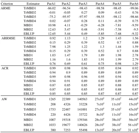
Hajek type of estimators (TrMBD1 and TrMBD3) under expected value model (14) are significantly large for all parameter choices. Further, high coverage rates under these estimators (TrMBD1 and TrMBD3) are the consequence of large biases and wider intervals (Table 1). These estimators are severely biased since under model calibration an appropriate estimator is HT type (Section 2). However, the HT type estimators (TrMBD2 and TrMBD4) derived under ratio and regression specifications for the expected value model are almost identical. Among conventional calibration weighting based MBD estimators, both Hajek type (MBD1) and HT type (MBD2) estimators are identical. Therefore, in further discussion we drop the Hajek type of estimator under model calibration and HT type estimator under classical calibration.

Table 1 shows that the average relative mean errors and the average relative RMSEs for TrMBD2 estimator are consistently lower than both MBD1 and EBLUP estimator for all choices of parameters. However, with same order of average relative mean errors, the relative RMSE of EBLUP estimator is lower order than MBD1. The average coverage rates for TrMBD2 estimator are relatively higher with smaller width of 2-sigma confidence intervals as compare to MBD1 and EBLUP. However, with almost same coverage rates, the EBLUP has smaller average widths than MBD1.

Figure 1-2 shows the region-specific performance measures generated by three estimators (TrMBD2, MBD1 and EBLUP) for simulation set-A. These results show that both the relative mean error and the relative RMSEs of TrMBD2 are smaller than MBD1 and EBLUP method in all regions. The relative biases and the RRMSE of MBD1 and EBLUP increases proportionately with non-linearity (ParA1 to ParA6). Figure 2 indicates that the coverage rate increases and the interval width decreases, hence accuracy increases in transformation-based methods. Further, the relative interval width under TrMBD2 reduced more rapidly as non-linearity in data increases. The results indicate a significant gain due to transformation based method of small area estimation for skewed data. Further, this gain is proportionate to non-linearity in the data. Between MBD1 and EBLUP methods, the EBLUP appears to perform better.

RMSEs of TrMBD2 method are lower than MBD1, but neither estimator dominates between TrMBD2 and EBLUP. The average coverage rates of EBLUP are higher than both MBD1 and TrMBD2. However, EBLUP has larger average widths than TrMBD2 (Table 2).

Figure 3-4 summarizes the region-specific performance measures generated by three estimators (TrMBD2, MBD1 and EBLUP) for simulation set-B. Figure 3 shows that for parameter set ParB1 and ParB5 (with quadratic rate γ = -1 and +1 respectively), the relative biases of TrMBD2 are larger than both MBD1 and EBLUP. However, for small values of γ (±0.5 i.e. near to zero), the relative biases are marginally same order for all methods. The relative RMSEs of TrMBD2 are lower than both MBD1 and EBLUP in most of the areas for all parameter sets except the parameter sets ParB2 and ParB3, where EBLUP is marginally better. Figure 4 demonstrates that although coverage rates of TrMBD2 are marginally lower for ParB2-ParB5 but interval widths are consistently smaller for all parameter choices (ParB1- ParB5). We noticed that in regional estimation loss in terms of coverage are marginal, however, gain in terms of reduced width is significant.

5.3.2 Design Based Simulations

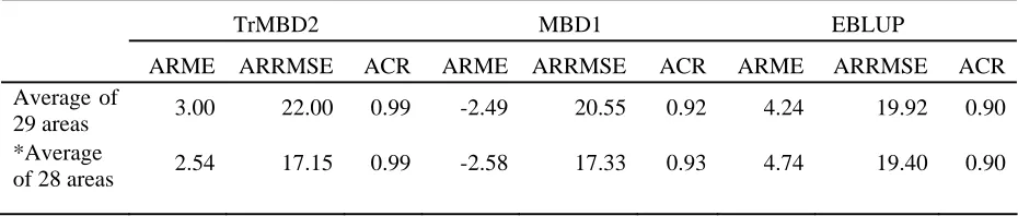
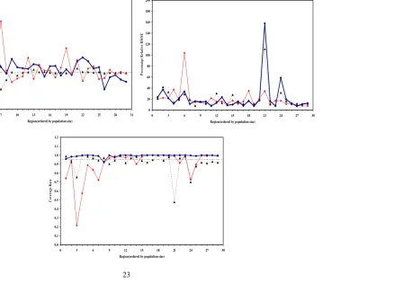
The results from the design-based simulation using the real data (AAGIS) show that the average relative bias of TrMBD2 is smaller than EBLUP and but larger than MBD1. The relative RMSE of TrMBD2 is marginally larger and the average coverage rate higher overall (Table 3). However, Figure 5 indicates that the high relative bias and RRMSE of TrMBD2 estimator is due to an outlier in region 21. The estimator TrMBD2 is more affected by this outlying point. If we discard the outlier contaminated estimates in region 21 and examine the average based on 28 regions then the TrMBD2estimator seems to be performing better. Overall transform variable based small area estimation methods for AAGIS data appears to provide efficient set of estimates.

6. Conclusions and Further Research

Our results show that transformed variable based method for small area estimation of skewed data performs well. We note that the gain in efficiency by accounting non-linearity in data via log transform linear model is quite significant, and thus we propose to use this method for small area estimation of skewed data. Further, even though assumed model deviates slightly from linearity on transform scale, the proposed method still works well with marginal gain. These results are based on normality assumption of random errors. However, we also investigated the method assuming a gamma distribution for the random errors and noticed that the form of the estimators remain the same. This indicates that method is robust with respect to distribution of random errors. The application of proposed SAE techniques to real data from AAGIS provides a satisfactory performance. The proposed method is advisable for skewed data but identification of appropriate transform model is crucial in application of this method, otherwise results can be misleading.

In the proposed method for SAE under log transform model, the survey variables only can have strictly positive values. However, the survey variables can take zero or negative values as well and therefore it would be useful to generalise the estimation procedure for skewed data that includes these cases. We are currently working on this issue, and results obtained so far are very encouraging.

Acknowledgement

The first author gratefully acknowledges the financial support provided by a PhD scholarship from the U.K. Commonwealth Scholarship Commission.

References

Bates, D.M. and Pinheiro, J.C. (1998). Computational Methods for Multilevel Models.

http://franz.stat.wisc.edu/pub/NLME/.

Carroll, R. and Ruppert, D. (1988). Transformation and Weighting in Regression. New York: Chapman and Hall.

Chambers, R.L. (1997). Weighting and Calibration in Sample Survey Estimation. Conference

on Statistical Science Honouring the Bicentennial of Stefano Franscini’s Birth (Editors C.

Malaguerra, S. Morgenthaler and E. Ronchetti). Basel: Birkhäuser Verlag.

Chambers, R.L. and Dorfman, A.H. (2003). Transformed Variables in Survey Sampling.

Southampton Statistical Sciences Research Institute, University of Southampton, U.K.,

WP/M03/21, http://www.s3ri.soton.ac.uk/publications.

Chandra, H. and Chambers, R.L. (2005). Comparing EBLUP and C-EBLUP for Small Area Estimation. Statistics in Transition, 7(3), 637-648.

Chen, G. and Chen, J. (1996). A Transformation Method for Finite Population Sampling Calibrated with Empirical Likelihood. Survey Methodology, 22, 139-146.

Deville, J.C. and Särndal, C.E. (1992). Calibration Estimators in Survey Sampling.

Journal of the American Statistical Association, 87, 376-382.

Harville, D.A. (1977). Maximum Likelihood Approaches to Variance Component Estimation and to Related Problems. Journal of the American Statistical Association, 72, 320–338. Karlberg, F. (2000). Population Total Prediction Under a Lognormal Superpopulation Model.

Metron, 53-80.

McCulloch, C.E. and Searle, S.R. (2001). Generalized, Linear, and Mixed Models. Wiley, New York.

Prasad, N.G.N. and Rao, J.N.K. (1990). The Estimation of the Mean Squared Error of Small Area Estimators. Journal of the American Statistical Association, 85, 163-171.

Rao, J.N.K. (2003). Small Area Estimation. New York: Wiley.

Royall, R.M. (1976). The Linear Least-Squares Prediction Approach to Two-Stage Sampling.

Journal of the American Statistical Association, 71, 657-664.

Royall, R.M. and Cumberland, W.G. (1978). Variance Estimation in Finite Population sampling. Journal of the American Statistical Association,73, 351-358.

[image:18.595.68.527.112.551.2]

Table 1 Average relative mean error (ARME), average relative RMSE (ARRMSE), average coverage rate (ACR) and average 2-sigma confidence interval width (AW) for simulation set-A

Criterion Estimator ParA1 ParA2 ParA3 ParA4 ParA5 ParA6 ARME TrMBD1 -86.02 -96.54 -98.43 -98.58 -98.45 -99.06

TrMBD2 -0.01 -0.05 0.27 0.09 -0.43 0.76

TrMBD3 -75.2 -95.97 -97.97 -98.55 -98.12 -98.66

TrMBD4 0.02 -0.07 0.28 0.11 -0.39 0.75

MBD1 10.98 4.11 -0.29 -6.28 -7.81 -9.59

MBD2 12.63 5.47 0.48 -5.91 -7.58 -9.5

EBLUP 12.65 5.44 0.49 -5.85 -7.68 -9.32

ARRMSE TrMBD1 0.92 1.13 1.2 1.29 1.43 1.56

TrMBD2 0.15 0.29 0.39 0.52 0.7 0.88

TrMBD3 7.98 1.25 1.22 1.3 1.44 1.59

TrMBD4 0.15 0.29 0.39 0.52 0.7 0.88

MBD1 1.03 1.47 1.79 1.89 1.98 2.78

MBD2 1.16 1.6 1.83 1.91 1.99 2.79

EBLUP 0.76 0.69 0.61 0.75 0.98 1.29

ACR TrMBD1 0.99 0.98 0.96 0.95 0.94 0.92

TrMBD2 0.94 0.9 0.89 0.89 0.89 0.89

TrMBD3 0.99 0.98 0.96 0.95 0.94 0.92

TrMBD4 0.94 0.91 0.89 0.89 0.89 0.89

MBD1 0.87 0.85 0.85 0.87 0.88 0.87

MBD2 0.87 0.85 0.85 0.87 0.88 0.87

EBLUP 0.85 0.85 0.85 0.87 0.87 0.87

AW TrMBD1 1265 22389 140563 27x104 35 x105 44x106

TrMBD2 208 4326 33228 7x104 11x105 15x106

TrMBD3 1753 22487 141001 27x104 35 x105 43x106

TrMBD4 220 4426 33722 8x104 11x105 16x106

MBD1 1007 19318 139346 28x104 38x105 56x106

MBD2 1033 19677 140626 28x104 38x105 56 x106

[image:19.595.73.526.108.298.2]

Table 2 Average relative mean error (ARME), average relative RMSE (ARRMSE), average coverage rate (ACR) and average 2-sigma confidence interval width (AW) for simulation set-B

Criterion Estimator ParB1 ParB2 ParB3 ParB4 ParB5

ARME TrMBD2 3.46 0.37 0.14 -0.9 -7.54

MBD1 -0.21 0.04 0.12 0.16 -0.85

EBLUP -0.19 0.04 0.13 0.17 -0.77

ARRMSE TrMBD2 0.35 0.33 0.33 0.34 0.39

MBD1 0.56 0.36 0.34 0.53 1.2

EBLUP 0.38 0.3 0.29 0.36 0.56

ACR TrMBD2 0.93 0.92 0.92 0.91 0.86

MBD1 0.91 0.92 0.92 0.92 0.9

EBLUP 0.93 0.94 0.94 0.93 0.92

AW TrMBD2 0.04 2.4 207 26409 5077959

MBD1 0.06 2.7 214 38660 12659988

EBLUP 0.05 2.6 214 33442 9929767

Table 3 Average relative mean error (ARME), average relative RMSE (ARRMSE) and average coverage rate (ACR) for AAGIS data

TrMBD2 MBD1 EBLUP

ARME ARRMSE ACR ARME ARRMSE ACR ARME ARRMSE ACR

Average of

29 areas 3.00 22.00 0.99 -2.49 20.55 0.92 4.24 19.92 0.90

*Average

of 28 areas 2.54 17.15 0.99 -2.58 17.33 0.93 4.74 19.40 0.90

[image:19.595.65.530.376.475.2]

Figure 1 Area-specific relative biases and RRMSE for simulation set-A ParA-1 -15 -10 -5 0 5 10 15 20

0 3 6 9 12 15 18 21 24 27 30

Region Number P e rcen ta g e R e la ti v e B ia s 0.0 0.5 1.0 1.5 2.0 2.5 3.0 3.5 4.0 P ercen ta g e Re la tiv

e RM

S E ParA-2 -15 -10 -5 0 5 10 15

0 3 6 9 12 15 18 21 24 27 30

Region Number P erce n ta g e R el a ti v e B ia s 0 1 2 3 4 5 6 7 8 P erc en ta g e Re la tiv

e RM

S E ParA3 -30 -25 -20 -15 -10 -5 0 5 10 15 20

0 3 6 9 12 15 18 21 24 27 30

Region Number P ercen ta g e R el a ti v e B ia s 0 1 2 3 4 5 6 7 8 P ercen ta g e Re la tiv e RM S E ParA-4 -35 -30 -25 -20 -15 -10 -5 0 5 10 15

0 3 6 9 12 15 18 21 24 27 30

Region Number P e rcen ta g e R e la ti v e B ia s 0 1 2 3 4 5 6 7 8 P ercen ta g e Re la ti v e RM S E ParA-6 -60 -50 -40 -30 -20 -10 0 10 20

0 3 6 9 12 15 18 21 24 27 30

Region Number P e rcen ta g e R e la ti v e B ia s 0 2 4 6 8 10 12 14 16 P erce n ta g e Re la tiv e RM S E ParA-5 -40 -35 -30 -25 -20 -15 -10 -5 0 5 10

0 3 6 9 12 15 18 21 24 27 30

[image:21.595.48.804.87.529.2]

Figure 2 Area-specific coverage rates and widths of CI for simulation set-A ParA-1 0.50 0.55 0.60 0.65 0.70 0.75 0.80 0.85 0.90 0.95 1.00

0 3 6 9 12 15 18 21 24 27 30

Region Number C ove ra ge R a te 0 250 500 750 1000 1250 1500 1750 2000 W idt h of 2-si g m a C o n fid en c e I n terv a l 0.50 0.55 0.60 0.65 0.70 0.75 0.80 0.85 0.90 0.95

0 3 6 9 12 15 18 21 24 27 30

Region Number C ove rage R a te 0 5000 10000 15000 20000 25000 30000 35000 40000 W idt h o f 2 -s ig m a C o n fid en ce In terv a l ParA-2 0.50 0.55 0.60 0.65 0.70 0.75 0.80 0.85 0.90 0.95

0 3 6 9 12 15 18 21 24 27 30

Region Number C ove rage R a te 20000 50000 80000 110000 140000 170000 200000 230000 260000 290000 W idt h o f 2 -s ig m a C o n fi d en ce I n terv a l ParA3 ParA-4 0.50 0.55 0.60 0.65 0.70 0.75 0.80 0.85 0.90 0.95

0 3 6 9 12 15 18 21 24 27 30

Region Number C ove rage R a te 50000 100000 150000 200000 250000 300000 350000 400000 450000 500000 550000 600000 W idt h o f 2 -s ig m a C o n fid en ce In terva l ParA-5 0.50 0.55 0.60 0.65 0.70 0.75 0.80 0.85 0.90 0.95

0 3 6 9 12 15 18 21 24 27 30

Region Number C ove rage R a te 0 1000000 2000000 3000000 4000000 5000000 6000000 7000000 8000000 W idt h o f 2 -s ig m a C o n fid en ce In terva l ParA-6 0.50 0.55 0.60 0.65 0.70 0.75 0.80 0.85 0.90 0.95

0 3 6 9 12 15 18 21 24 27 30

[image:22.595.48.800.83.520.2]

Figure 3 Area-specific relative biases and RRMSE for simulation set-B ParB-1 -15 -10 -5 0 5 10

0 3 6 9 12 15 18 21 24 27 30 Region Number P e rc en ta g e R e la ti ve B ia s 0.2 0.4 0.6 0.8 1.0 1.2 1.4 1.6 Pe rc e n ta g e R e la tive R M S E ParB-2 -8 -6 -4 -2 0 2 4

0 3 6 9 12 15 18 21 24 27 30

Region Number P ercen ta g e R el a ti v e B ia s 0.25 0.30 0.35 0.40 0.45 0.50 0.55 0.60 P ercen ta g e Re la ti v

e RM

S E ParB-3 -10 -8 -6 -4 -2 0 2 4

0 3 6 9 12 15 18 21 24 27 30

Region Number P ercen ta ge R el a ti ve B ia s 0.20 0.25 0.30 0.35 0.40 0.45 0.50 0.55 0.60 P ercen ta g e Re la ti v

e RM

S E ParB-4 -8.0 -6.0 -4.0 -2.0 0.0 2.0 4.0

0 3 6 9 12 15 18 21 24 27 30

Region Number P ercen ta g e R el a ti v e B ia s 0.25 0.35 0.45 0.55 0.65 0.75 0.85 0.95 1.05 1.15 1.25 P ercen ta g e Re la ti v

e RM

S E ParB-5 -30 -25 -20 -15 -10 -5 0 5 10

0 3 6 9 12 15 18 21 24 27 30

[image:23.595.52.796.109.543.2]

Figure 4 Area-specific coverage rates and widths of CI for simulation set-B ParB-1 0.50 0.55 0.60 0.65 0.70 0.75 0.80 0.85 0.90 0.95 1.00

0 3 6 9 12 15 18 21 24 27 30

Region Number C o v era ge R a te 0.03 0.04 0.05 0.06 0.07 0.08 0.09 0.10 W idt h of 2-si g m a C o n fid en ce In terv a l ParB-2 0.50 0.55 0.60 0.65 0.70 0.75 0.80 0.85 0.90 0.95 1.00

0 3 6 9 12 15 18 21 24 27 30

Region Number C o ve rage R a te 2 2.2 2.4 2.6 2.8 3 3.2 3.4 W idt h o f 2 -s ig m a C o n fid en ce I n terv a l 0.50 0.55 0.60 0.65 0.70 0.75 0.80 0.85 0.90 0.95 1.00

0 3 6 9 12 15 18 21 24 27 30

[image:24.595.157.723.86.556.2]

Figure 5 Area-specific relative biases and RRMSE for AAGIS data

-40 -20 0 20 40 60 80

1 4 7 10 13 16 19 22 25 28 31

Region(ordered by population size)

P

ercen

ta

g

e R

el

a

ti

v

e B

ia

s

0 20 40 60 80 100 120 140 160 180 200

0 3 6 9 12 15 18 21 24 27 30

Region(ordered by population size)

P

er

ce

n

at

ge

R

el

a

ti

ve

R

M

S

E

0.0 0.1 0.2 0.3 0.4 0.5 0.6 0.7 0.8 0.9 1.0 1.1 1.2

0 3 6 9 12 15 18 21 24 27 30

C

ove

rage

R

a