Further developments in the conflation of CFD and building simulation

FURTHER DEVELOPMENTS IN THE CONFLATION OF CFD

AND BUILDING SIMULATION

Beausoleil-Morrison I

, Clarke J A

, Denev J

Macdonald I A

, Melikov A

, Stankov P

(2) ESRU, University of Strathclyde, Scotland, [email protected]

(3) Technical University of Sofia, Bulgaria, [email protected]

(4) Centre for Indoor Environment and Energy, Technical University of Denmark, [email protected]

ABSTRACT

To provide practitioners with the means to tackle problems related to poor indoor environments, building simulation and computational fluid dynamics can usefully be integrated within a sin-gle computational framework.

This paper describes the outcomes from a research project sponsored by the European Com-mission, which furthered the CFD modelling aspects of the ESP-r system. The paper sum-marises the form of the CFD model and describes the method used to integrate the thermal and flow domains.

Ke ywords: Building performance simulation, computational fluid dynamics, integrated mod-elling.

INTRODUCTION

Within building energy simulation two modelling approaches are extant: nodal networks and com-putational fluid dynamics.

Within the former method, as implemented within the ESP-r system (Clarke and Hensen 1991), the building and its air handling plant are treated as a collection of nodes representing rooms (or parts of rooms), equipment connection points, ambient conditions etc. Inter-nodal con-nections are then defined to represent components such as cracks, doors, windows, fans, ducts, pumps etc. Each component is assigned a model that gives the mass flow rate as a function of pres-sure difference. Consideration of the conserva-tion of mass at each node leads to a set of non-lin-ear equations that can be integrated over time to characterise the flow domain.

Although well adapted for building energy application, the nodal network method is limited when it comes to consideration of indoor comfort and air quality: because momentum effects are neglected, intra-room air movement cannot be studied; and, as a result of the low resolution, local surface convection heat transfer is poorly

represented. To overcome these limitations, it is necessary to introduce a CFD model.

The CFD method is based on the solution of the conservation equations for mass, momentum and energy at discrete points within a room. For a given boundary condition, numerical methods are employed to solve for the mean time temperature, pressure and velocity fields. It is also possible to determine the distribution of water vapour or pol-lutants, and to assess the mean age (freshness) of air at different locations within the room. Such information is the prerequisite of an appraisal of indoor air quality and discomfort.

MODEL DESCRIPTION

In recent years the application of CFD to build-ings—a non-steady, mixed flow (turbulent, lami-nar and transitional) problem—has grown signifi-cantly (Nielsen 1989 & 1994, Jones and Whittle 1992, Denev and Stankov 2000a) and attempts have been made to combine CFD and building energy models (Negra ˜o 1995) or to extend CFD to include building features (Schild 1997). A building-integrated CFD model comprises six aspects: domain discretisation; a set of equations to represent the conservation of energy, mass, momentum and species; the imposition of bound-ary conditions; an equation solver; a method to link the CFD, building thermal and network air flow models; and the interpretation of results. The following sections describe the treatment of these aspects within the ESP-r system.

DOMAIN DISCRETISATION

into a number of regions, here 3 in the x-direction and 2 in the z-direction (the y-direction is not shown). These regions are then gridded using a constant or variable spacing evaluated from

xi=L(i/n)c

where xi is the co-ordinate of grid linei, L the

overall dimension of the region, n the number of

grid lines and c a power law coefficient. Where

c> 1, the grid starts fine and becomes course asi

increases, with c< 1 defining the opposite

sce-nario.

grid decreasing at boundary z

y

z

x x

Rx1 Rx2 Rx3

Rz2

Rz1

i increasing Figure 1: Room discretisation.

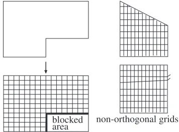
The scheme of table 1 has been implemented to control the gridding process. For the case of non-orthogonal geometries (figure 2), or where inter-nal obstructions are present, the technique may be applied to an orthogonal bounding box but with the boundary of the non-participating cells treated as solid surfaces and assigned a boundary condi-tion. To further accommodate the range of com-monly encountered room shapes, the z-direction may be made non-orthogonal (Denev and Stankov 2000b).

blocked

area non-orthogonal grids

Figure 2: Treatment of non-orthogonal geometries.

CONSERVA TION EQUATIONS

The movement of air within a room may be deter-mined from the solution of the discretised mass, energy and momentum equations when subject to given boundary conditions. While these equa-tions can be solved directly or by the technique of

Large Eddy Simulation (Deardorff 1970, David-son and Neilsen 1996), this is a computationally non-trivial task because these techniques required a fine mesh size to resolve the turbulent fluctua-tions. The turbulence transport technique (Rodi 1980) is therefore used whereby the instantaneous values of temperature, concentration, velocity, pressure etc may be represented as the sum of their mean and fluctuating components, and the effect of turbulent motion time-averaged. Using tensor notation, this gives rise to the following mean conservation equation for an incompressible fluid:

∂ ∂t(ρφ)=

∂ ∂xi

 Γφ_∂∂φ_x

i

−ρUiφ_+Sφ (1)

whereφ is a transport variable such as continuity

(φ=1), enthalpy, concentration of contaminant or

velocity; ρ the density (kg m−3), Γ_φ a diffusion

coefficient,Ui a mean velocity component (U, V,

W), and S_φ a mean source term. The transport

variables, diffusion coefficients and source terms are then as given in table 2 for each conservation equation type.

The effect of turbulent motion on the mean

flow is modelled by the standard k−ε model

which is widely used because of its computational stability and reasonable accuracy (Launder and Spalding 1972 & 1974, Chen 1995). Its function

is to determine the eddy viscosity,µt, of table 2 at

each grid point as a function of local values of the

turbulence kinetic energy (k) and its rate of

dissi-pation (ε):

µt =ρCµ k2

ε

whereC_µis an empirical coefficient.

The equations for k andε are also cast in the

form of eqn (1), with the diffusion and source

terms as given in table 2. Because the k and ε

equations contain experimentally derived

parame-ters, the standard k−ε model is fully valid only

for cases of fully turbulent shear layer flow and free jets. As described later, a zero-equation (mixing length) model (Chen and Xu 1998) is used as the basis of an exploratory simulation, commissioned at each time-step, to assist with the

appropriate configuring of the k−ε model. This

model has shown good agreement with experi-mental data for three test cases: natural convec-tion with infiltraconvec-tion, forced convecconvec-tion, and mixed convection with displacement ventilation

(Srebric et al 1999). Its attractiveness is that it

does not require the solution of thekandε

equa-tions in order to calculate the eddy viscosity.

Instead, µt is directly related to the local mean

computational burden but with the retention of reasonable accuracy in many applications (Beau-soleil-Morrison 2000).

At near-wall regions where viscous effects pre-dominate and the flow is laminar, logarithmic (log-law) wall functions are employed with the

k−ε model whereby the form of the velocity and

temperature profile within the boundary layer is assumed in order to determine the surface shear stress and convective heat transfer (Launder and Spalding 1974). Improving this aspect of CFD is the aim of Low Reynolds Number models (Lam

and Bremhorst 1981, Chien 1982, Patel et al

1985, Stankov and Denev 1996) with enhanced treatment of buoyancy effects (Ince and Launder 1989).

Since this convective heat transfer constitutes the pivot point between the air flow and thermal domains, any inaccuracy in its treatment will affect the entire simulation (Beausoleil-Morrison and Clarke 1998). For this reason, and depending on the outcome from the exploratory CFD run, the log-law wall functions are replaced—either by empirical heat transfer coefficients or by more applicable wall functions (e.g. for vertical walls undergoing buoyancy driven flow wall functions

by Yuanet al(1993) are used).

Equations (1) may be discretised by standard methods to obtain a set of linear equations of the form

apφp = i

Σ

whereφ is the relevant variable of state, p

desig-nates a domain cell of interest, i designates the

neighbouring cells and b relates to the source

terms applied at p.

The problem therefore reduces to the solution of a set of time-averaged nodal conservation

equations for U, V, W, H, C, k and ε. Because

these equations are strongly coupled and highly non-linear—that is the equation coefficients and source terms are dependent on the state vari-ables—they are solved iteratively for a given set of boundary conditions. Moreover, within an integrated simulation, the equation-sets corre-sponding to the building thermal, network air flow and CFD models must be solved together.

BOUNDARY CONDITIONS

Initial values of ρ,Uiand Hare required at time

t=0 for all domain cells. For solid surfaces, the

temperature (or flux) at points adjacent to the domain cells is required. For cells subjected to an in-flow from ventilation openings and

doors/win-dows, the mass/momentum/ energy/ species

exchange must be given in terms of the

distribution of relevant variables of state—U,V,

W,H,k,ε andC. At outlets, the normal practice

is to impose a constant pressure, and the

condi-tions ∂Un

/

∂ε

/

to the boundary. Within an integrated simulation, these data can be determined from the solution of equations corresponding to the building thermal and network flow models.

SOLUTION PROCEDURE

The SIMPLE-Consistent (SIMPLEC; Van Door-mal and Raithby 1984) method is used to solve the flow equations. This method is similar to the SIMPLE (Semi-Implicit Method for Pressure-Linked Equations) method (Patankar 1980) but has less onerous simplifications applied to the momentum/continuity equations in order to obtain the pressure field correction. It is therefore more accurate.

Essentially, the pressure of each domain cell is linked to the velocities connecting with surround-ing cells in a manner that conserves continuity. The method then accounts for the absence of an equation for pressure by establishing a modified form of the continuity equation to represent the pressure correction that would be required to ensure that the velocity components determined from the momentum equations move the solution towards continuity. This is done by using a guessed pressure field to solve the momentum equations for intermediate velocity components

U, V andW. These velocities are then used to

estimate the required pressure field correction

from the modified continuity equation. The

nature of this modifications, and the simplifica-tions applied in the process, are detailed else-where (Versteeg and Malalasekera 1995). The energy equation, and any other scalar equations (e.g. for concentration), are then solved and the process iterates until convergence is attained. To avoid numerical divergence, under relaxation is applied to the pressure correction terms. The con-centration distribution data is then post-processed to obtain the local mean age of air (freshness) using the method of Sandberg (1981).

Where the CFD domain is connected to a flow network, both solvers operate in tandem with iter-ation used to handle the case of strong interac-tions.

EQUATION-SET LINKING

The solvers for the building thermal, HVAC, net-work air flow and CFD equations act

co-opera-tively. This required a conflation controller

CFD model is appropriately configured at each time-step.

At the start of a time-step, the zero-equation turbulence model is employed in investigative mode to determine the likely flow regimes at each surface. The eddy viscosity distribution to result

is then used to initialise the k and ε fields and a

second simulation performed for the time-step. This process repeats at each computational time-step.

The nature of the flow at each surface is evalu-ated from the local Grashof (Gr) and Reynolds (Re) Numbers as determined from the investiga-tive simulation. The Grashof Number (the ratio of the buoyancy and viscous forces) indicates how buoyant the flow is adjacent to the surface, while the Reynolds Number (the ratio of the inertial and viscous forces) indicates how forced is the flow. The following conditions are relevant:

Gr/ Re2<< 1: forced convection effects

over-whelm free convection.

Gr/ Re2>> 1: free convection effects dominate.

Gr≈Re2: both forced and free convection effects

are significant.

Based on the outcome, the following procedure is invoked.

Where buoyancy forces are insignificant, the buoyancy term in the z-momentum equation is dropped to improve solution convergence.

Where free convection predominates, the

log-law wall functions are replaced by the Yuanet al

(1993) wall functions and a Dirichlet† boundary

condition imposed where the surface is vertical; otherwise a convection coefficient correlation is

prescribed and a Neumann† boundary condition

imposed (this means that the thermal domain will influence the flow domain but not the reverse).

Where convection is mixed, the log-law wall functions are replaced by a prescribed convection

coefficient and a Robin† boundary condition

imposed.

Where forced convection predominates, the ratio of the eddy viscosity to the molecular

vis-cosity (µt/µ), as determined from the

investiga-tive simulation, is examined to determine how tur-bulent the flow is locally:

µt/µ ≤30:- the flow is weakly turbulent; the

log-law wall functions are replaced by a prescribed convection coefficient and a Neumann boundary condition is imposed;

µt/µ > 30:- the log-law wall functions are

retained and a Dirichlet boundary condition is † Dirichlet condition: fixed temperatureθ=θs.

Neumann condition: fixed heat fluxk∂θ ∂n=q. Robin condition: heat flux proportional to the

local heat transferk∂θ

∂n=hc(θ−θs).

imposed.

The iterative solution of the flow equations is initiated for the current time-step. For surfaces

wherehccorrelations are active, these are shared

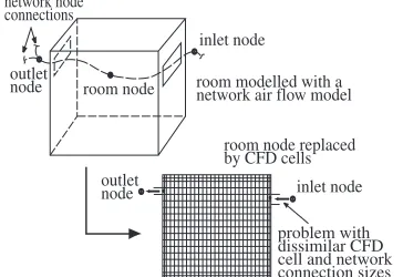
with the building model so that the surface heat flux is imposed on the CFD solution. Where such correlations are not active, the CFD-derived con-vection coefficients are inserted into the building model’s surface energy balance equations. Where an air flow network is active, the network node representing the room is removed and new network connections are added to effect a cou-pling with the appropriate domain cell(s) (Negra ˜o

1995, Clarkeet al1995) as shown in figure 3. A

special device has been established to ensure the accurate representation of both mass and momen-tum exchange between domain cells and network flow components of dissimilar size (Denev 1995). The appropriate network connection’s area is increased or reduced to achieve a match with the corresponding domain cell(s) and then the associ-ated velocity is adjusted to maintain the correct flow rate. Within the solution process, the adjusted velocity is imposed as a boundary condi-tion to satisfy the flow rate and then it is read-justed in the momentum equation to give the cor-rect momentum. From the viewpoint of the flow network, the air exchanges with the CFD domain are treated as sources or sinks of mass at appro-priate points within the flow network solution.

room node outlet

node

inlet node

inlet node outlet

node network node connections

room modelled with a network air flow model

room node replaced by CFD cells

problem with dissimilar CFD cell and network connection sizes

Figure 3: Coupling network flow and CFD models.

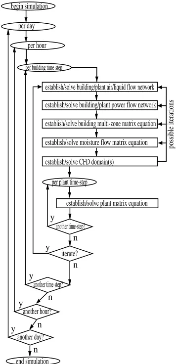
The foregoing procedure is embedded within a higher level controller that acts to synchronise the customised solvers for the building, HVAC, net-work flow and CFD equation-sets (figure 4). Note that the frequency of inv ocation of these solvers may differ. For example, in order to reduce the computational burden, the building-side solver can be invoked less frequently than the HVAC

solver. Note also that that iteration may be

invoked to resolve problematic coupling between domain.

It is also possible to operate on the basis of

building model might comprise several zones, with only a subset addressed by CFD. At the same time, a flow network may be linked to one or more CFD domains, have nodes in common with some, but not all, of the other zones compris-ing the buildcompris-ing model and have extra nodes to represent zones and/or plant components that are outwith the modelled building portion. Each part of such a model would then operate on the basis of best available information (e.g. a zone with no matched air flow model would utilise its user-specified infiltration/ventilation rates).

RESULTS INTERPRETATION

On the basis of the multi-variate outputs from an integrated simulation, the spatial and temporal variation of indoor air quality and thermal dis-comfort may be assessed according to standards prENV 1752, ISO EN 7730 and ANSI/ASHRAE 55-1992. Such an assessment is based on a set of relevant indicators:

1. the variation in vertical air temperature between floor and head height;

2. the absolute temperature of the floor; 3. radiant temperature asymmetry; 4. unsatisfactory ventilation rate;

5. unsatisfactoryCO2level;

6. local draught assessed on the basis of the turbu-lence intensity distribution;

7. additional air speed required to off-set an ele-vated temperature;

8. comfort check based on effective temperature. 9. mean age of air.

Figure 5 gives an example output showing the distribution of air mean age for a 2D room slice. Taken together, the above outputs allow indoor regions to be differentiated in terms of air temper-ature, radiant asymmetry, humidity, contaminant level and air freshness, with various composite indices used to quantify standards of perfor-mance.

CONCLUSIONS

The CFD module of the ESP-r integrated mod-elling package has been refined as part of a col-laborative research project funded by the Euro-pean Commission (ERB IC15 CT98 0511) with inputs from related projects. These refinements were concerned with the treatment of complex geometries, blockages (furnishings, equipment etc), buoyancy, ventilation openings, surface heat transfer and the assessment of the spatial and tem-poral variation of thermal comfort and indoor air quality.

ACKNOWLEDGEMENTS

The authors are indebted to the European Com-mission for their invaluable support, and to our project colleagues who serviced the validation

aspects of the project (Bartaket al2001).

REFERENCES

Bartak M, Cermak M, Clarke J A, Denev J, Drkal F, Lain M, Macdonald I A, Majer M and Stankov P 2001 Experimental and numerical study of local

mean age of air Proc. Building Simulation 2001

(Rio de Janeiro)

Beausoleil-Morrison I 2000 The Adaptive Cou-pling of Heat and Air Flow Modelling within

Dynamic Whole-Building SimulationPhD Thesis

(Glasgow: University of Strathclyde)

Beausoleil-Morrison I and Clarke J 1998 The

Implications of Using the Standard k−ε

Turbu-lence Model to Simulate Room Air Flows which

are not Fully Turbulent Proc. ROOMVENT ’98

99-106 (Stockholm)

Chien K-Y 1982 Predictions of Channel and Boundary-Layer Flows with a

Low-Reynolds-Number Turbulence Model AIAA Journal 20₍₁₎

33-8

Clarke J A, Dempster W M and Negra ˜o C 1995 The Implementation of a Computational Fluid Dynamics Algorithm within the ESP-r System Proc. Building Simulation ’95166-75 (Madison) Clarke J A and Hensen J L M 1991 An Approach to the Simulation of Coupled Heat and Mass

Flows in BuildingsIndoor Air3_283-96

Chen Q 1995 Comparison of Different k−ε

Models for Indoor Air Flow Computations Numerical Heat TransferB_{(28) 353-69}

Chen Q and Xu W 1998 A Zero-Equation Turbu-lence Model for Indoor Airflow Simulation Energy and Buildings28_{(2) 137-44}

Davidson L and Neilsen P V 1996 Large Eddy Simulations of the Flow in a Three-Dimensional

Ventilated RoomProc. ROOMVENT ’962_161-8

(Yokohama)

Deardorff J W 1970 A Numerical Study of Three-Dimensional Turbulent Channel Flow at Large

Reynolds NumbersJ. Fluid Mech. 42_453-80

Denev J A 1995 Boundary conditions related to near-inlet regions and furniture in ventilated

roomsProc. Application of Mathematics in

Denev J A and Stankov P 2000a Indoor climate assessment using computer simulation of air flow

in a ventilated room Journal of Theoretical and

Applied Mechanics31₍₁₎

Denev J A and Stankov P 2000b Non-Orthogonal Grid Generation Techniques Applied to Room

Airflow Modeling Proc. 26th Summer School on

Applications of Mathematics in Engineering and Economics (Sozopol)

Ince N Z and B E Launder 1989 On the computa-tion of buoyancy-driven turbulent flows in

rectan-gular enclosuresInt. J. Heat and Fluid Flow10₍₂₎

110-7

Jones P J and Whittle G E 1992 Computational fluid dynamics for building air flow prediction

-current status and capabilitiesBuilding and

Envi-ronment21_{(3) 321-38}

Lam C K G and Bremhorst K A 1981 Modified

form of the k−ε model for predicting wall

tur-bulenceJ. of Fluids Engng103_456-60

Launder B E and Spalding D B 1972

Mathemati-cal Models of Turbulence(New York: Academic) Launder B E and Spalding D B 1974 The

Numer-ical Computation of Turbulent Flows Computer

Methods in Applied Mechanics and Engineering3 269-89

Negra ˜o C O R 1995 Conflation of computational fluid dynamics and building thermal simulation PhD Thesis(Glasgow: University of Strathclyde) Nielsen P V 1989 Airflow Simulation Techniques

Progress and Trends Proc. 10th AIVC Conf.

203-23

Nielsen P V 1994 Air Distribution in

Rooms-Research and Design MethodsProc. ROOMVENT

’94Krakow, Poland, V1, 15-35.

Patankar S V 1980 Numerical heat transfer and

fluid flow(Hemisphere)

Patel V C, Rodi W and Scheuerer G 1985 Turbu-lence models for near-wall and low Reynolds

number flows: A review AIAA Journal 23

1308-19

Rodi W 1980 Turbulence Models and their Appli-cations in Hydraulics—A State of the Art Review (Delft: Int. Association for Hydraulic Research) Sandberg M 1981 What is ventilation efficiency? Building and Environment16_123-35

Schild P 1997 Accurate Prediction of Indoor

Cli-mate in Glazed Enclosures PhD Thesis

(Trond-heim: Norwegian University of Science and Tech-nology)

Srebric J, Chen Q and Glicksman L R 1999 Vali-dation of a Zero-Equation Turbulence Model for

Complex Indoor Airflow Simulation ASHRAE

Tr ans.105₍₂₎

Stankov P and Denev J 1996 Turbulence mod-elling of low Reynolds number effects in 3D

ven-tilated roomsProc. HERMIS’96 695-702 (Athens)

ISBN 960-85176-5-6

Versteeg H K and Malalasekera W 1995 An intro-duction to Computational Fluid Dynamics: The Finite Volume Method (Harlow, England: Long-man)

Yuan X, Moser A and Suter P 1993 Wall Func-tions for Numerical Simulation of Turbulent

Nat-ural Convection Along Vertical PlatesInt. J. Heat

Mass Transfer36_{(18) 4477-85}

per day

per hour

per building time-step

establish/solve building/plant air/liquid flow network

establish/solve building multi-zone matrix equation

per plant time-step

establish/solve plant matrix equation

iterate? begin simulation

another time-step?

another time-step?

another hour?

another day?

end simulation y

n

n

n

y n

establish/solve CFD domain(s)

n y

establish/solve moisture flow matrix equation establish/solve building/plant power flow network

y

y

possible iterations

Figure 5: Distribution of the local mean age of air.

Table 1: Domain gridding parameters.

Number of grid lines in region Po wer law coefficient

n > 0 c = 1n cells distributed uniform distribution

over the region

n < 0 c > 1|n| cells distributed increasing grid size†

symmetrically over the region

c < 1 decreasing grid size†

†_{From the beginning to the end (or middle if n < 0) of the region.}

Table 2: Transport variables (φ), diffusion coefficients (Γφ) and source terms (Sφ).

Equation Type φ Γφ Sφ

Continuity 1 -

-Momentum ui µef −

∂p

∂xi −ρgi

Energy H ΓT SH

Species C ΓC SC

Turbulent kinetic energy k µef

σk

G−CDρε−Gb

Dissipation rate ofk ε µef

σε

C1 ε

kG−C2ρ

ε2

k −C3

ε

kGb

ΓT=

µ

Pr +

µt

σT

; ΓC=

µ

Sc +

µt

σC

; µef =µt+µ ; ρ=ρ(T,C)

Gb=g_βT

µt

σT ∂T

∂xi +βC

µt

σC ∂C

∂xi 

 ; G=µt_ ∂ui ∂xj

+∂uj ∂xi  

∂ui ∂xj

CD=1. 0 ; C1=1. 44 ; C2=1. 92 ; σk=1. 0 ; σε =1. 3 ; σT=0. 9 ; σC=0. 9

whereµis molecular viscosity (kg m−1_s−1_),µ

tis eddy viscosity,Pis pressure (N m−2),gthe

gravi-tational acceleration (m s−2),Cpthe specific heat (J kg−1K−1),q′′′is heat generation (W m−3),Pris

the Prandtl Number,Scis the Schmidt Number,σkis the turbulent energy diffusion coefficient,σε

is the turbulent energy dissipation diffusion coefficient,σTis the turbulent Prandtl Number,σCis