Kernel methods for short-term spatio-temporal wind prediction

Kernel Methods for Short-term Spatio-temporal

Wind Prediction

Jethro Dowell, Stephan Weiss and David Infield

Glasgow, UK

Email: [email protected]

Abstract—Two nonlinear methods for producing short-term spatio-temporal wind speed forecast are presented. From the relatively new class of kernel methods, a kernel least mean squares algorithm and kernel recursive least squares algorithm are introduced and used to produce 1 to 6 hour-ahead predictions of wind speed at six locations in the Netherlands. The perfor-mance of the proposed methods are compared to their linear equivalents, as well as the autoregressive, vector autoregressive and persistence time series models. The kernel recursive least squares algorithm is shown to offer significant improvement over all benchmarks, particularly for longer forecast horizons. Both proposed algorithms exhibit desirable numerical properties and are ripe for further development.

I. INTRODUCTION

Wind energy penetration is increasing on power systems around the world driven primarily by a desire to reduce reliance on carbon intensive alternatives. To optimally utilise variable renewable generation, such as wind power, power systems, and the way they are operated, are changing: trans-mission networks must connect distant renewable generation to load centres, distribution networks must accommodate small scale generation, and operators must consider the stochas-tic nature of this new variable generation when performing scheduling tasks [1]–[4]. Decisions relating to scheduling tasks are informed by forecasts on a variety of temporal and spatial scales, and the upper limit on the level of variable generation that can be accommodated by power systems will ultimately be set by the skill of these forecasts (and their users).

This paper is concerned with short-term wind speed fore-casting, a key input when predicting wind power. Unlike day-ahead forecasting, where numerical weather predictions are essential, short-term forecasts (up to approximately 6 hours) produced by purely statistical methods are superior to complex physical models [5]. Spatio-temporal approaches, which model and forecast multiple locations simultaneously to capture space-time dependencies, have been shown to improve skill significantly when compared to forecasts which only consider individual locations.

To date, the majority of statistical methods used for wind speed prediction have been linear despite the well established nonlinear nature of the wind. We therefore explore a relatively new and exciting class of learning algorithms called kernel methods which enable the linear processing of nonlinear ‘features’. This approach retains many desirable properties of linear processing, such as fast learning algorithms and

the existence of a unique optimal solution, while making it possible to capture some nonlinearities.

Over the last decade, many kernel methods have been developed and now represent a distinct class of learning algorithms. Such methods are based on the so called ‘kernel trick’, a result which allows the inner product of a nonlinear function defined by a Mercer kernel (Mercer’s Theorem [6]) to be calculated while the function itself remains unknown [7]. This has advantageous properties in function estimation and classification; support vector machines, for example, rely on kernel methods.

A direct application of nonlinear function estimation is regression, where some nonlinear mapping is followed by linear processing in a high (or infinite) dimensional feature space. The kernel trick removes the need to identify the mapping associated with the a given Mercer kernel which may not be available or be difficult to calculate; the only challenge is selecting an appropriate kernel for the problem at hand.

Several linear methods have been ‘kernelised’ including the popular least means squares (LMS) [8] and recursive least squares (RLS) [9] algorithms, plus extensions, [10]–[13] for example. Reported applications to forecasting include high frequency wind prediction [13], [14] and load forecasting [15], among others.

In this paper we examine the application of two kernel methods to the short-term wind forecasting problem: a simple kernelised LMS algorithm and the kernel RLS of [9] are studied. The theory of Kernel methods is briefly introduced in Section II and the prediction problem is stated in III followed by descriptions of the KLMS and KRLS algorithms in III-B and III-C, respectively. A case study is then presented in Section IV, including how the algorithms and benchmarks were implemented, and their performance is evaluated. Finally, conclusions are drawn in Section V.

II. KERNELMETHODS

Kernel methods are a class of learning algorithm which use Mercer kernels in order to produce nonlinear versions of conventional linear learning algorithms. The kernel trick allows the inner product of two input vectors in some high-dimensional Hilbert space_H(often called the feature space) to be calculated without explicit knowledge of the feature vectors, which form a the nonlinear projection of the input vectors in

First we introduce the Mercer kernel, a continuous, sym-metric, positive-definite function k: X × X → R, X ∈ Rn

(orCn). Mercer’s theorem states that any Mercer kernelk(·,·)

can be expressed as the inner product of some fixed nonlinear function_{φ(x) :_{X → H}1, x∈ X },

k(xi,xj) =hφ(xi), φ(xj)i_H1 , (1) where _H1 is a real- or complex-valued reproducing kernel Hilbert space, for which k(_·,_·) is a reproducing kernel and

h·,_·iH1 is the corresponding inner product in_H1.

Equation (1) states that ifxiandxjare mapped ontoH1by φ(xi)andφ(xj), respectively, then the inner product of these functions can be calculated by evaluating the kernelk(xi,xj), even if the mappingφ(_·)is unknown. This result is known as the Kernel trick.

The Gaussian kernel is frequently used in real world appli-cations with particular success in time series prediction prob-lems. It is the expansion function for an infinite dimensional feature space and is given by

k(xi,xj) = exp −||xi−xj||2 (2)

and used throughout this study [7]. While other kernels could be chosen, the Gaussian kernel has a physical interpretation as a measure of similarity, which is fitting here, and has out performed other candidate kernels (triangular and polynomial) in other similar work [9], [13]. The choice, or construction, of kernels is very much an open problem and the subject of ongoing research.

III. PREDICTIONALGORITHMS

A. Prediction Set-up

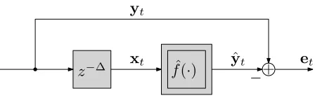
The prediction problem is outlined in Fig. 1, whereby the purpose of a potentially nonlinear function f(_·)is to look ∆ samples ahead in time, estimating y_t∈Rn (or Cn) from the

input vector xt ∈ Rm (or Cm) containing space-time data

comprising measurements y_t−∆, y_t−∆−1, .... The predictor is written

y_t=f(xt) . (3)

The aim in the context of a prediction problem is to find an estimatefˆ(_·)of f(_·)which minimises the estimation error in the mean squared sense, i.e.

J =X

t

|et|2=

X

t

|y_t−fˆ(xt)|2 (4)

The linear approximation of this problem is given byfˆ(xt) = Axt where A ∈ Rn×m (or Cn×m) is a coefficient matrix

whose entries are to be determined. Many estimation schemes based on this approximation have been studied.

Alternatively, we can state the approximation in terms of the mapping φ(_·) to place us in a nonlinear setting, writing

ˆ

f(xt) = Aφ(xt) with A ∈ Rn×l (or Cn×l). The

proper-ties of Mercer kernels make it possible to derive estimation schemes forf(_·)in a highl-dimensional feature space without

ˆ

f

(

_·

)

x

y

ˆ

z

₊

y

e

−

Fig. 1. Nonlinear systemf(·)set-up to predict the vector quantityytsome ∆samples ahead based on inputxt.

performing calculations in such a space. This combines sim-ple imsim-plementation of linear methods with the advantageous properties of working with a nonlinear mapping.

In the remainder of this section two popular linear al-gorithms are discussed, the least mean squares (LMS) and recursive least squares (RLS) algorithms, are presented in their conventional linear and kernelised forms. Since we are only concerned with real valued wind speed, the proceeding sec-tions assume all quantities are real valued and the conjugasec-tions necessary in the complex case are omitted.

B. Kernel LMS

The LMS algorithm comprises an update scheme based on gradient descent for the coefficient matrix Agiven by

A0 = 0n×m (5)

et = yt−Atxt (6) At+1 = At+µetxTt , (7)

where the prediction yˆ_t = Atxt and µ is the positive learning rate which controls the trade-off between confidence in individual samples and convergence speed.

When kernelised, the update step (7) becomes

At+1=At+µetφT(xt) , (8)

however to express the algorithm in terms of inner products it is more convenient to wright

At+1=µ t

X

i=1

eiφT(xi) , (9)

which allows the prediction to be expressed as

ˆ y_t=µ

t

X

i=1

eiφT(xi)φ(xt) . (10)

Finally, ifφ(·)is chosen to be an expansion function of some reproducing kernel Hilbert space, the inner product in (10) can be computed using the corresponding generating kernelk(_·,_·), i.e.

ˆ y_t=µ

t

X

i=1

eik(xi,xt) . (11)

sparsity constraint, by retaining a finitedictionary,D, of input vectors. At each time step t the input vector is compared to the dictionaryDt−1; if the minimum distance betweenxtand Dt−1 exceeds some sparsity parameter ν, it is added to the dictionary, i.e. Dt := Dt−1∪ {xt}, else Dt := Dt−1. The estimation is now

ˆ

y_t=µ X i∈Dt−1

eik(xi,xt) . (12)

C. Kernel RLS

The RLS algorithm attempts to minimise the cost function (4) at each time step, rather than the mean squared error as in the LMS algorithm. The cost function is rewritten as

J(w) =

t

X

i=1

(yi−Aφ(xi))2=|Yt−ΦTtw|2 , (13)

whereYtandΦtare output and projected input data matrices, and w is a weight vector. As before, working in some high dimensional feature space is undesirable, so writing the optimal weight vector aswt=Pt_i=1αiφ(xi) =Φtαwe use the kernel trick to express the cost function as

J(α) =|Yt−Ktα|2 , (14)

where[Kt]i,j =k(xi,xj); i, j= 1, ..., t, is called the kernel matrix.

In theory the minimiser α =K−t1Yt could be computed recursively using the conventional RLS algorithm, however, as with the kernalised LMS algorithm, the complexity of the calculation would increase with each new sample, in addition to possible over-fitting when the number of samples becomes large. We therefore sparsify the algorithm by retaining a finite dictionary of samples and replacing Kt with the dictionary kernel matrix[ ˜Kt]i,j =k(xi,xj); i, j ∈D, andαt with the reduced weights α˜t.

The derivation of the KRLS algorithm is lenghthy and involved, and space here is limited so the update steps are stated without proof. The full derivation, and pseudo code of its implementation, can be found in the original paper [9].

Initialisation: K˜1 = [k(x1,x1)], K˜−11 = [1/K˜1], α˜1 =

[y1/K˜1],P1= [1], sparsity parameter:ν. fort=2,3,...

Compute:k˜t−1(xt)where[˜kt−1(xt)]i=k(xi,xt), i∈D

Make Prediction:yˆ_t= ˜kT_t−1(xt) ˜α Compute:at= ˜K−t−11k˜t−1(xt) Compute:δt=k(xt,xt) + ˜k

T

t−1(xt)at

Case 1: The new sample is approximately linearly inde-pendent with respect to the current dictionary, satisfying

δt > ν, therefore the new sample, xt, is added to the dictionary. The matricesK˜−t1,Pt andα˜tare updated as follows:

˜

K−t1 =

1

δt

_˜

K−_t−1₁+ataTt −at −aT

t 1

(15)

Pt =

Pt−1 0 0T ₁

(16)

˜ αt =

"

˜

αt−1−a_δtt(yt−k˜

T

t−1(xt)at) 1

δt(yt−

˜

kT_t−1(xt)at)

#

(17)

Case 2:The new sample is approximately linearly dependent with respect to the current dictionary, satisfyingδt≤ν, so the new sample is not added to the dictionary andK˜−t1=

˜

K−t−11. The matricesPtandα˜t are updated as follows:

Pt = Pt−1−Pt−1

ataTtPt−1

1 +aT

tPt−1at

(18)

q_t def= Pt−1at 1 +aT

tPt−1at

(19)

˜

αt = α˜t−1+ ˜K−t1qt

y_t−k˜T_t−1(xt)at

(20)

end

D. Sparsity

Both the KLMS and KRLS algorithms retain a dictionary of input samples as a sparse representation of the complete history of input samples up to some time. It is an important property of the dictionary that it is finite, and it can be shown to be so with only mild conditions on the data and kernel function. Ifx_{∈ X} andφ(x)_{∈ H} then if _X is compact, and the sparsity parameter is positive (ν >0), the dictionary will be finite. For a rigorous proof, see [9].

It should be noted that for these algorithms to be fully adaptive they should incorporate some forgetting mechanism whereby out-of-date dictionary elements are ‘forgotten’ in order track changing dynamics of the process being modelled. A sophisticated multi-kernel LMS algorithm is developed [13] which includes this feature, as well as the ability to combine multiple kernel functions. The drawback, of course, is the need to determine the parameters for each of these mechanisms.

IV. CASESTUDY

A. Test Data

This transformation aids spatial prediction by removing biases present at individual measurement locations that would otherwise interfere with the spatio-temporal correlation of the data. The procedure is simple to implement once information regarding the terrain surrounding a weather station is known.

B. Implementation

The KLMS and KRLS are employed to predict the wind speed at the six locations which are embedded in the vector y_{t ∈} R6. The input vector x∆|t for a ∆ = 1 step-ahead prediction is the concatenation of plagged values of y_t, i.e. x1|t = (yTt−1, ...,yTt−p)T, and for horizons of ∆ > 1 where not all lags are available, predictions are used such that

x∆|t=



        

ˆ y_{∆−1|t−1}

.. . ˆ y_1|t−∆+1

y_t−∆ .. . y_t−p



        

, (21)

whereyˆ_∆|tdenotes the prediction ofy_tmade∆steps ahead. This is the so calleddirect forecastingapproach. In this study we are only concerned with forecast horizons up to 6 hours, or∆ = 1, ...,6and the forecasts for each horizon are made in parallel by distinct predictors. The number of temporal lags is a trade off between accuracy and computational expense, for the KLMS p= 6 and KRLSp= 3since the improvement in accuracy was negligible for greater values.

The sparsification parameter and LMS learning rate are determined heuristically by exhaustive search to minimise the residual error on the training data. The sparsification parameter is ν = 0.02 for the KRLS and ν = 0.1 for the KLMS. The KLMS learning rate was chosen to beµ= 0.01.

C. Benchmarks

An important benchmark is the persistence forecast which supposes that the future wind speed will be the same as the most recent measurement. While its implementation is trivial its performance is still considered acceptable by many practitioners, particularly in situations where more complex approaches offer only modest gains. The persistence forecast ∆-hours ahead is given by

ˆ

y_∆|t=y_t−∆ . (22)

In order to compare the kernelised algorithms to conven-tional techniques and highlight the value of spatial informa-tion, two non-recursive linear time series models are used as further benchmarks in addition to the conventional LMS and RLS algorithms. The first is the non-spatial autoregressive (AR) model which is given by

ˆ

y∆|t=

∆−1

X

i=1

aiyˆ∆−i|t−i+ p

X

i=∆

aiyt−i (23)

for each location. The number of lags p is determined by the Akaike information criterion, and the parameters ai are

determined by maximum likelihood estimation assuming in-dependent identically distributed (i.i.d) Gaussian prediction errors.

The second is the vector generalisation of AR, the vector autoregressive model (VAR). As in the multivariate kernelised algorithms, the measurements at multiple locations are embed-ded in the vectory_tand the model is written

ˆ

y_∆|t=Ax∆|t , (24)

wherext is given by Equation (21). Once again the number of lags p is determined by the Akaike information criterion and assuming i.i.d Gaussian errors the coefficient matrixA_∈ Rn×np is determined by maximum likelihood estimation.

The conventional LMS algorithm, with update scheme given in equations (5)–(7) and learning rate µ = 0.0005, and conventional RLS with update scheme

et = yt−Atxt (25)

kt =

xT

tQt

1/λ+xT

tQtxt

(26)

Qt+1 = Qt−Qtxtkt (27) At+1 = At+etkt , (28)

and forgetting factor λ = 0.9995 are also included for comparison with their kernelised versions. The look-ahead indexing has been dropped here to avoid notational clutter but the principle still applies.

The AR and VAR methods are non-recursive, that is to say that their parameters are estimated directly from the training data and are then fixed throughout the test period. The other methods, with the exception of persistence, are recursive and as such are initialised and then run sequentially through the training and test data, updating their parameter estimates at each step.

D. Results

Performance is evaluated in terms of root mean squared error, which is given by the expression

RMSE∆=

v u u t1

T T

X

t=1

(ˆy∆|t−yt)2 (29)

for the samples y1, ..., yT in the test dataset at each location and for each forecast horizon∆ = 1, ...,6.

The performance of the kernelised algorithms and bench-marks is illustrated in Figure 2 in terms of mean RMSE accross the six sited in the dataset. The most simplistic approaches, persistence and AR perform significantly worse at all forecast horizons than the more sophisticated VAR, RLS and KRLS. Both the LMS and its kernalised version (KLMS) have intermediate performance, reflective of their complexity, though the KLMS performs particularly poorly for the 1 and 2 hour ahead predictions.

Forecast Horizon [hours]

RMSE [

m

s

−

1 ]

1 2 3 4 5 6

0.5

1.0

1.5

2.0

2.5

3.0 _AR VAR KRLS KLMS Persistence

Fig. 2. Mean root mean squared error across all 6 sites for Kernelised algorithms and benchmarks.

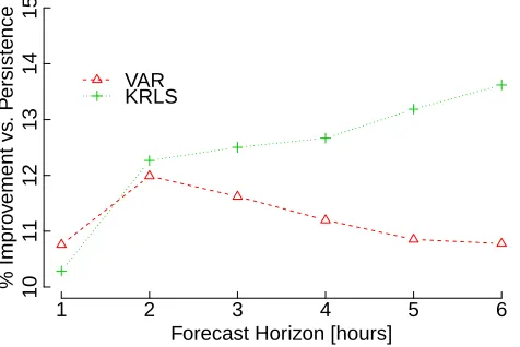
Forecast Horizon [hours]

% Impro

v

ement vs

. P

ersistence

1 2 3 4 5 6

10

11

12

13

14

15

VAR KRLS

Fig. 3. Percentage improvement vs. persistence for the VAR and KRLS forecasts.

outperforms the two linear methods for the longer horizons. It is also notable that the KLMS improves relative to the LMS at longer forecast horizons. In both cases the kernelised versions of linear algorithms offer improved 5 and 6 hour ahead predictions.

V. CONCLUSIONS

For the short-term spatio-temporal prediction of wind speed, we have presented two examples from a new class of learning algorithms called kernel methods. The kernel least mean squares and kernel recursive least squares algorithms are non-linear extensions of their conventional non-linear forms and have been applied to a dataset comprising wind speed measurements made at six locations in the Netherlands over a period of 2 years. The KRLS in particular shows significant improvement over several established linear benchmarks, especially for longer forecast horizons.

ACKNOWLEDGEMENTS

The authors gratefully acknowledge the Royal Netherlands Meteorological Institute for their supply of meteorological data, and the support of the UK’s Engineering and Physical Sciences Research Council via the University of Strathclyde’s Wind Energy Systems Centre for Doctoral Training, grant number EP/G037728/1.

REFERENCES

[1] S. J. Watson, L. Landberg, and J. A. Halliday, “Application of wind speed forecasting to the integration of wind energy into a large scale power system,” IEE Proceedings—Generation, Transmission and Dis-tribution, vol. 141, no. 4, pp. 357–362, 1994.

[2] E. Denny and M. O’Malley, “Wind generation, power system operation, and emissions reduction,”IEEE Transactions on Power Systems, vol. 21, no. 1, pp. 341–347, 2006.

[3] E. Bitar, R. Rajagopal, P. Khargonekar, K. Poolla, and P. Varaiya, “Bringing wind energy to market,”IEEE Transactions on Power Systems, vol. 27, no. 3, pp. 1225–1235, 2012.

[4] S. Faias, J. De Sousa, F. Reis, and R. Castro, “Assessment and opti-mization of wind energy integration into the power systems: Application to the portuguese system,”IEEE Transactions on Sustainable Energy, vol. 3, no. 4, pp. 627–635, 2012.

[5] G. Giebel, R. Brownsword, G. Kariniotakis, M. Denhard, and C. Draxl,The State-of-the-Art in Short-Term Prediction of Wind Power. ANEMOS.plus, 2011, project funded by the European Commission under the 6th Framework Program, Priority 6.1: Sustainable Energy Systems.

[6] J. Mercer, “Functions of positive and negative type, and their connection with the theory of integral equations,” Philosophical Transactions of the Royal Society of London, Series A, vol. 209, no. 441–458, pp. 415–446, 1909.

[7] B. Schølkopf and A. J. Smola,Learning with Kernels: Support Vector Machines, Regularization, Optimization, and Beyond. MIT Press, 2001.

[8] W. Liu, P. Pokharel, and J. Principe, “The kernel least-mean-square algorithm,” IEEE Transactions on Signal Processing, vol. 56, no. 2, pp. 543–554, Feb 2008.

[9] Y. Engel, S. Mannor, and R. Meir, “The kernel recursive least-squares algorithm,” IEEE Transactions on Signal Processing, vol. 52, no. 8, pp. 2275–2285, Aug 2004.

[10] W. Liu, I. M. Park, Y. Wang, and J. Principe, “Extended kernel recursive least squares algorithm,” IEEE Transactions on Signal Processing, vol. 57, no. 10, pp. 3801–3814, Oct 2009.

[11] S. Van Vaerenbergh, M. Lazaro-Gredilla, and I. Santamaria, “Kernel recursive least-squares tracker for time-varying regression,” IEEE Transactions on Neural Networks and Learning Systems, vol. 23, no. 8, pp. 1313–1326, Aug 2012.

[12] F. A. Tobar, A. Kuh, and D. P. Mandic, “A novel augmented complex valued kernel LMS,” in 7th Sensor Array and Multichannel Signal Processing Workshop. Hoboken, NJ, USA: IEEE, June 2012. [13] F. Tobar, S.-Y. Kung, and D. Mandic, “Multikernel least mean square

algorithm,” IEEE Transactions on Neural Networks and Learning Systems, vol. 25, no. 2, pp. 265–277, Feb 2014.

[14] A. Kuh, C. Manloloyo, R. Corpuz, and N. Kowahl, “Wind prediction using complex augmented adaptive filters,” inInternational Conference on Green Circuits and Systems, June 2010, pp. 46–50.

[15] C. Liu and F. Liu, “The short-term load forecasting using the kernel recursive least-squares algorithm,” in 3rd International Conference on Biomedical Engineering and Informatics, vol. 7, Oct 2010, pp. 2673–2676.