One-loop Feynman integrals with Carlson hypergeometric functions

One-loop Feynman integrals with Carlson hypergeometric

functions

Khiem HongPhan1,∗

1_{VNUHCM-University of Science, 227 Nguyen Van Cu, Dist. 5, Ho Chi Minh City, Vietnam.}

Abstract. In this paper, we present analytic results for scalar one-loop two-, three-, four-point Feynman integrals with complex internal masses. The calcu-lations are considered in general space-time dimensionDfor two- and three-point functions andD ₌ 4 for four-point functions. The analytic results are expressed in terms of the Carlson hypergeometric functions (R-functions) and valid for both real and complex internal masses.

1 Introduction

In order to confront particle physics theory with high-precision of experimental data at future colliders, theoretical predictions including high-order corrections are required. In general framework for computing high-order corrections, detailed calculations for one-loop multi-leg and higher-loop are necessary for building blocks. When we compute scattering processes which Feynman diagrams involve internal unstable particles that can be on-shell, we have to resume Feynman propagators with a complex mass term in the denominator. In other words, one has to perform the perturbative renormalization in the Complex-Mass Scheme [1]. Therefore, the calculations for Feynman loop integrals with complex internal masses are of great interest. Furthermore, within the general framework for computing two-loop or higher-loop corrections scalar one-higher-loop integrals in general space-time dimension play a crucial role for several reasons. Higher-terms in theε-expansion from one-loop integrals are necessary for building blocks. In additional, one-loop integrals at higher space-time dimensionD>4 may be taken into account in the framework.

There have been available many calculations for scalar one-loop integrals inD₌4−₂ε

dimensions atε0_{-expansion [2–11]. Scalar one-loop integrals in general dimensionDhave} performed in [12–16]. However, not all of these calculations cover general dimensionDwith a generalε-expansion at general scale and complex internal masses. In this paper, based on the method in [5–8], we present analytic results for scalar one-loop two-, three-, four-point Feynman integrals with complex internal masses. The calculations are considered in general space-time dimension D for two- and three-point functions and D = 4 for four-point functions. The analytic results are expressed in terms of the Carlson hypergeometric functions.

The layout of the paper is as follows: In section 2, we present in detail the method for evaluating scalar one-loop functions. In this section, analytic results for one-loop two-, three-and four-point functions are presented. Conclusions three-and outlooks are devoted in section 3. Several useful formulas used in this calculation can be found in the appendix.

∗

2 The calculations

Based on the method introduced in Refs. [5–7], we present the calculations for scalar one-loop functions with complex internal masses. Scalar one-one-loopN-point functions are defined

JN =

Z

dDl 1

P₁P₂· · · P_N. (1)

Where inverse Feynman propagators are given

P_{k = (}l+qk)2−m2_k+iρ, with k=1,2,· · ·,N. (2)

The Feynman prescription isiρ. We use momentaqk=Pkj=1pj,pjare external momenta and they are inward as shown in Fig. 1. The internal masses in the Complex-Mass scheme are taken the form of

m2_k=m2_0k−_{im0kΓk, for Γk}>₀. (3)

The Γk are decay widths of unstable particles. The momenta qk may take the following configuration

q1=q1(q10,q11,0,· · ·,0, − →

0D−J), (4)

q2=q2(q20,q21,0,· · ·,0, − →

0D−J), (5)

q3=q3(q10,q31,q32,0,· · ·,0, − →

0D−J), (6)

· · ·₌· · · ,

qN−1=qN−1(q(N−1)0,q(N−1)1,· · ·,q(N−1)(J−1), − →

0D−J) (7)

which haveJnon-zero components. Here,q10 =0 forq2₁ <0 andq11 =0 forq2₁ >0. As a result, scalar product of external and internal momenta are obtained

q2_k = q2_k0−q_k2₁− · · · −q2_k(J−1), (8)

l2 ₌ l2₀−l₁2− · · · −l2_J−1−l 2

⊥, (9)

l·_{qk = l0}·_qk0−_l1·_qk1· · · −_lJ−1·_{qk(J−1). (10)}

In parallel space which is the linear span of the external momenta and its orthogonal space (POS) [5, 6], scalar one-loopN-point functions are taken the form of:

JN =

2πD−2J

Γ(D−J₂ ) ∞

Z

−∞

dl0dl1· · ·dlJ−1 ∞

Z

0

dl⊥

lD−J−1 ⊥

P₁P₂· · · P_N. (11)

The propagators now become

P_{k = (}l0+qk0)2−(l1+qk1)2− · · · −(lJ−1+qk(J−1))2−l2⊥−m 2

k+iρ, (12)

fork = 1,2,· · ·,N. The calculations can be summarized as follows. We first make the partition for the integrand ofJNas

1

P₁P₂· · · P_N = N

X

k=1

1

P_k N

Q

l₌1 k,l

(P_l− P_k)

pN−1 pN

p1

p2 p3

p4 m2

1 m2

2 m2

3

m2

N

m2

N−1

Figure 1.Generic Feynman diagrams at one-loop

withNexternal lines. All external momenta are inward and follow momentum conservation

qN=PN

j=1pj=0.

with

P_l− P_{k = (}l0+ql0)2−(l0+qk0)2+(l1+ql1)2−(l1+qk1)2

+· · ·₊₍lJ−1+ql(J−1))2−(lJ−1+qk(J−1))2+m2k−m 2

l (14)

= alkl0+blkl1+· · ·+clklJ−1+d˜lk. (15)

Where we have introduced the following kinematic variables

alk = 2(ql0−qk0), blk=−2(ql1−qk1), · · ·, (16)

clk = −2(ql(J−1)−qk(J−1)), d˜lk=q2_l −q2_k+m2_k−m2_l. (17)

Making a shift

l0→l0+qk0, l1→l1+qk1,· · ·, lJ−1 →lJ−1+qk(J−1), (18)

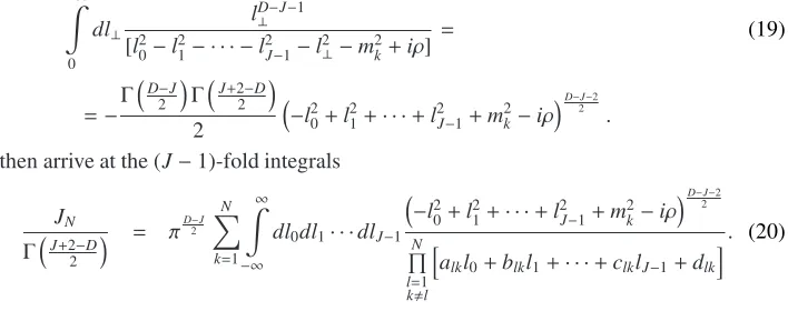
we convert allP_{kin (13) to}P_{N. As a matter of this fact, the}l⊥-integral then yields a simple form which can be taken easily as follows:

∞

Z

0

dl⊥

lD−J−1 ⊥ [l2

0−l 2

1− · · · −l 2 J−1−l

2

⊥−m2k+iρ]

= (19)

=−Γ

_D−J

2

ΓJ+22−D

2

−l2₀+l2₁+· · ·₊l2_J−1+m2_k−iρ

D−J−2 2

.

We then arrive at the (J−_{1)-fold integrals}

JN

ΓJ+2−D 2

= π

D−J 2

N

X

k=1 ∞

Z

−∞

dl0dl1· · ·dlJ−1

−_l2 0+l

2

1+· · ·+l 2 J−1+m

2 k−iρ

D−₂J−2

N

Q

l=1 k,l

h

alkl0+blkl1+· · ·+clklJ−1+dlk

i

. (20)

In this formulaalk,blk,· · ·,clk ∈Randdlk=(ql−qk)2−(m_l2−m2_k)∈ Cwhich is obtained from ˜dlkafter applying the shift (18). The integrals in (20) can be carried out with the help of residue theorem. For that purpose, one first linearizes thel0for example, .i.el′₁=l1+l0. The result reads

JN

ΓJ+2−D 2

= π

D−J 2

N

X

k=1 ∞

Z

−∞

dl0dl1· · ·dlJ−1

−_2l0l1+l2

1+· · ·+l 2 J−1+m

2 k−iρ

D−₂J−2

N

Q

l₌1 k,l

h

ABlkl0+blkl1+· · ·+clklJ−1+dlk

i

(21)

⊗ · · · ⊗

⊗

l1>0

⊗ ⊗ ⊗ · · · ⊗

⊗

l1<0

⊗ ⊗

Figure 2.We close the contour integration forl0that the poles in (22) locate outside the contour.

withABlk=alk−blk. The singularity poles of the integrand in (21) are obtained:

l0 =

l2

1+· · ·+l 2 J−1+m

2 k−iρ 2l1

, Im(l0)=−

m0kΓk+ρ 2l1

, (22)

and

l(₀l) = −blkl1+· · ·+clklJ−1+dlk

ABlk

, Im[l(₀l)]=Im − dlk

ABlk

!

. (23)

The polel0in (22) locates upper (lower) inl0-complex plane ifl1 <0 (l1 >0) respectively. We plan to close the contour integration forl0thatl0-poles in (22) locate outside the contour, seen Fig. 2 for more detail. As a result, the poles in (23) are only taken into account to the residue contributions forl0-integration. The resulting reads

JN

ΓJ+22−D

= π

D−J 2

N

X

k=1 N

X

l=1 k,l

          

f_lk+

∞

Z

0

dl1+flk− 0 Z −∞ dl1            · · · ∞ Z −∞

dlJ−1[1−δ(ABlk)] (24)

×

"

1−₂ blk

ABlk

!

l2

1+· · ·+l 2 J−1−2

clk

ABlk

l1lJ−1−2

dlk

ABlk

l1+m2_k−iρ

#D−₂J−2

N

Q

m=1 m,k m,l

h

˜

Amlkl1+· · ·+C˜mlklJ−1+F˜mlk

i

.

Where theδ-function is defined as

δ(x)=       

0, if x,_0;

1, if x₌0. (25)

New kinematic variables ˜Amlk,· · ·,C˜mlk ∈Rand ˜Fmlk ∈Care obtained from residue contri-butions of the poles in (23). The functions f_lk±indicate the location of the poles in (23) in the

l0complex plane:

f_lk+=                         

0, if Im − dlk

ABlk

!

<0;

1, if Im − dlk

ABlk

!

=0;

2, if Im − dlk

ABlk

!

>0.

and f_lk−=                         

0, if Im − dlk

ABlk

!

>0;

1, if Im − dlk

ABlk

!

=0;

2, if Im − dlk

ABlk

!

<0.

q2 _q2

m2₁ m2₂

b b _{Figure 3.Bubble diagrams.}

We continue to linearizel1 in numerator of the integrand of (24) by applying a Euler shift

l1 →l1+βlkl2.βlkcan be chosen in such a way of the disappearance ofl21-term. The residue theorem is applied against forl1-integration. At the final stage, the resulting integrals can be expressed in terms ofR_{-functions [18] which is defined as}

∞

Z

r

(x−r)α−1 k

Y

i₌1

(zi+wix)−bidx

=B₍β−α, α)R_α−β b1,· · ·,bk,r+

z1

w1

,· · ·,r+ zk

wk

! k

Y

i=1

w−bi

i , (27)

withβ ₌Pk

i=1bi. In next subsections, we present analytic results for scalar one-loop two-, three- and four-point functions. Detailed calculations for these functions have published in Ref. [17].

2.1 One-loop two-point functions

In POS,J2takes the form of [5, 6]

J2= 2πD2−1

ΓD−21

∞

Z

−∞

dl0 ∞

Z

0

dl⊥

lD−2 ⊥ [(l0+q10)2−l2⊥−m21+iρ][l

2 0−l

2

⊥−m22+iρ]

. (28)

Hereq = q(q10, − →

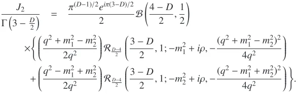
0D−1) for q2 > 0. Ifq2 < 0, we refer [17] for detailed evaluations. The results in [17] have shown that the below formulas forJ2are valid for both above cases. The R_{-function representation for two-point integrals is as follows [17]:}

J2

Γ3−D

2

=

π(D−1)/2_eiπ(3−D)/2

2 B

4−D

2 , 1 2

!

(29)

×

(      

q2

+m2

1−m 2 2 2q2

     

RD−4 2

     

3−D

2 ,1;−m 2 1+iρ,−

(q2

+m2

1−m 2 2)

2

4q2

     

+      

q2−_m2 1+m

2 2 2q2

     

RD−4 2

     

3−D

2 ,1;−m 2 2+iρ,−

(q2−_m2 1+m

2 2)

2

4q2

      )

.

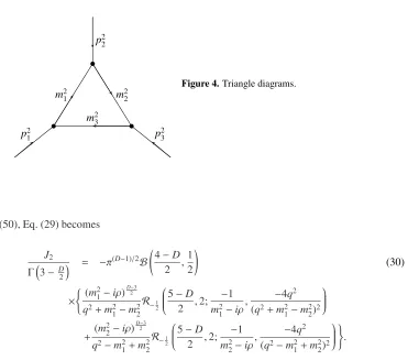
p2 2

p2₁ p2₃

m2 3

m2₁ m2₂

b b

b

Figure 4.Triangle diagrams.

(50), Eq. (29) becomes

J2

Γ3−D

2

= −π

(D−1)/2_B 4−D 2 ,

1 2

!

(30)

×

(_(m2

1−iρ) D−3

2

q2_+m2 1−m

2 2

R₋1 2

     

5−D

2 ,2; −₁

m2₁−_iρ,

−₄q2

(q2_+m2 1−m

2 2)

2

     

+(m

2 2−iρ)

D−3 2

q2_−m2 1+m

2 2

R₋1 2

     

5−D

2 ,2; −₁

m2 2−iρ

, −4q

2

(q2_−m2 1+m

2 2)

2

      )

.

It can be seen that the right hand sides of Eqs. (29,30) are symmetric under the interchange ofm2₁ ↔ m2₂. From Eqs. (29,30) we can take the limits of m₁2 = m2₂ → _{0 and} q2 → ₀ respectively, seen Ref. [17] for more detail.

2.2 One-loop three-point functions

The momenta q1,q2 take the following configuration q1 = q1(q10,q11, − →

0D−2), q2 =

q2(q20,q21, − →

0D−2). Here q10 = 0 forq2₁ < 0 andq11 = 0 forq2₁ > 0. The results for J3 in this paper cover both the above cases. The integralJ3in POS takes the form of [5, 6]

J3 =

πD−22

ΓD−22

∞

Z

−∞

dl0 ∞

Z

−∞

dl1 ∞

Z

−∞

l⊥D−3dl⊥

1

[(l0+q10)2−(l1+q11)2−l2⊥−m2₁+iρ]

× 1

[(l0+q20)2−(l1+q21)2−l2⊥−m22+iρ][l 2 0−l

2 1−l

2

⊥−m23+iρ]

. (31)

follows [17]

J3

Γ2−D

2

= −π

D

2_iB₍₄−D,1) 3

X

k=1 3

X

l=1 k,l

[1−δ(ABlk)]

Amlk

(αlk−iρ) D−4

2

×

(

S+_lk f_lk+R_D−4 4−D 2 ,

4−D

2 ,1;+Z (1) lk ,+Z

(2) lk,+Fmlk

!

(32)

+S−_lk f_lk−R_D−4 4−D 2 ,

4−D

2 ,1;−Z (1) lk ,−Z

(2) lk ,−Fmlk

!)

,

form, l. When all internal masses are real, f+ lk = f

−

lk = 1 andS ±

lk =1, Eq. (32) confirms the results of, for instance,J3in the Eq. (11) of [6]. We can derive other represents forJ3by applying several transformations forR_{-functions, as shown in appendix. For example, with} the help of (50), one obtains

J3

Γ2−D

2

= −π

D

2iB(4−D,1) 3

X

k₌1 3

X

l₌1 k,l

[1−δ(ABlk)]

Cmlk

(m2_k)(D−4)/2 (33)

×

      

f_lk+R₋₁

      

6−_D 2 ,

6−_D 2 ,2;+

1

Z(1)_lk ,+

1

Z(2)_lk ,+

1

Fmlk

      

−f_lk−R−1

      

6−_D 2 ,

6−_D 2 ,2;−

1

Z_lk(1),

− 1

Z_lk(2),

− 1

Fmlk

             

,

form,l. The kinematic variables appear in subsection are listed:

alk = 2(ql0−qk0), blk = −2(ql1−qk1),

ABlk = alk−blk, clk = (qk−ql)2+m2_k−m2_l,

Amlk = −ABkmblk+ABlkbkm, Cmlk = −ABkmclk+ABlkckm,

Fmlk = Cmlk/Amlk, Z_lk(1,2) = _aclk lk+blk

±

q clk

alk+blk

2

−m2k−iρ

αlk .

The factorS±

lkis given

S±_{lk = Exp}hπiθ(−αlk)θ[∓_Im(Z_lk(1))]θ[∓_Im(Z(2)_lk)] (D−₄₎i

×_Exph−_{πiθ(αlk)θ[}±_Im(Z(1)

lk )]θ[±Im(Z (2)

lk )] (D−4)

i

. (34)

We turn our attention into the analytic results for scalar one-loop four-point functions in next subsection.

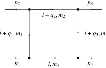
2.3 One-loop four-point functions

At present, the calculations for four-point functions are performed in D = 4. We set configuration of external momenta as follows q1 = (q10,q11,0,0), q2 = (q20,q21,0,0),

q3 = (q30,q31,q32,0). Where q10 = 0 forq21 < 0 andq11 = 0 forq21 > 0. Our result presented in this paper cover all the above cases. In POS,J4takes the form of

J4=2 ∞

Z

−∞

dl0dl1dl2 ∞

Z

0

dl⊥ 1

P₁P₂P₃P₄, (35)

withP_{k =(l+qk)}2_−m2

p2

p1

p3

p4 l,m4

l₊q2,m2

l+q1,m1 l+q3,m3

b

b

b

b

Figure 5.Box diagrams.

written as one-fold integrals [17] as follows

J4

iπ2 = 4

X

k₌1 4

X

l₌1 k,l

4

X

m₌1 m,l m,k

1−δ(AClk)1−δ(Bmlk)

AClk(BmlkAnlk−BnlkAmlk)

× ₍₃₆₎

×

        

∞

Z

0

dz G(z)

"

(f_lk+g+_mlk+f_lk−g+_mlk) ln Fnmlk

βmlk

!

−f_lk+g+_mlkln z+Fnmlk

βmlk

!

−_f+ lkg

− mlkln −

z+Fnmlk

βmlk

!

−_(f−

lkg+mlk+flk+g+mlk) ln

S(σmlk,z)

Pmlkz+Qmlk

!

+f_lk+g+_mlkln S(σmlk=0,z)

Pmlkz+Qmlk

!

+f_lk+g−_mlkln −S(σmlk=0,z)

Pmlkz+Qmlk

! #

+

0

Z

−∞

dz G(z)

"

−f_lk+g−_mlkln −Fnmlk

βmlk

!

+(f_lk−g−_mlk+f_lk−g+_mlk) ln z+Fnmlk

βmlk

!

−f_lk−g−_mlkln Fnmlk

βmlk

!

−₍f_lk−g+_mlk+ f_lk−g−_mlk) ln S(σmlk=0,z)

Pmlkz+Qmlk

!

+f_lk−g−_mlkln S(σmlk,z)

Pmlkz+Qmlk

!

+f_lk+g−_mlkln − S(σmlk,z)

Pmlkz+Qmlk

! # )

Where the related kinematic variables are given:

alk = 2(ql0−qk0), blk = −2(ql1−qk1),

clk = −2(ql2−qk2), dlk = (ql−qk)2−(m2l −m 2 k),

AClk = alk+clk, αlk = blk/AClk,

Amlk = amk−_AClkalk ACmk, Bmlk = bmk−_AClkblk ACmk,

Cmlk = dmk−_ACdlk

lkACmk, Dmlk =

−₄₍ql−qk)2/AC2_lk,

Fnmlk = C_AnlkBmlk−BnlkCmlk nlkBmlk−BnlkAmlk

±iρ′_{, β}(1,2) mlk =

Amlk Bmlk−αlk

±

s

Amlk Bmlk−αlk

2 −Dmlk

Dmlk ,

Qmlk = −2

_C

mlk Bmlk

−₂ dlk AClk

βmlk, Pmlk = −2

_A

mlk Bmlk

−αlk−βmlkDmlk

,

withσmlk =0,−11/βmlk. TheS(σmlk,z) andG(z) are obtained:

S(σmlk,z) = S_mlk(σ)z2+(Emlk+Qmlkσmlk)z−m2_k+iρ, (37)

G−1(z) = Zmlkz2+Kmlkz−βmlk(m2k−iρ)−FnmlkQmlk, (38)

withZmlk =Dmlkβmlk−PmlkandKmlk =Emlkβmlk−Qmlk−PmlkFnmlk. The functionsf_lk±(and

g±

mlk) are defined as in (26) with replacingclk/ABlkbydlk/AClk(andCmlk/Bmlk) respectively. TheJ4in (36) is decomposed into two basic integrals as follows:

I_{1 =} ∞

Z

0

1 (z+T1)(z+T2)

dz₌R−1(1,1;T1,T2), (39)

I_{2 =} ∞

Z

0

ln(1+z/T3) (z+T1)(z+T2)

dz= (40)

= lim

ω→0 1

ω

        

∞

Z

0

1 (z+T1)(z+T2)

dz− ∞

Z

0

(1+z/T3)−ω (z+T1)(z+T2)

dz

        

(41)

= lim

ω→0 1

ω

(

R₋₁₍₁,1;T1,T2)−

B₍₁₊ω,1)

T₃−ω R−1−ω(1,1, ω;T1,T2,T3)

)

. (42)

The ε-expansions for allR_{-functions appear in this paper have devoted in Ref. [17]. The} numerical checks for all analytic formulas in this paper and applications of this work to compute Feynman diagrams in real scattering processes have shown in [17].

3 Conclusions

We have presented the analytic results for scalar one-loop two-, three-, four-point Feynman integrals with complex internal masses. The analytic results in this paper are valid for both real and complex internal masses. The calculations have carried out in general space-time dimension for two- and three-point functions. At present work, the four-point functions have performed inD =4. The analytic formulas have expressed in terms of theR_{-functions. In} future work, we will extend this work to tensor one-loop integrals (to be published).

Acknowledgment: This work is funded by Vietnam’s National Foundation for Science and Technology Development (NAFOSTED) under the grant number 103.01-2016.33. The au-thor is grateful to the organizers of ISMD 2018 for the invitation and for financial support.

Appendix: Useful relations for

R

_-functions

Useful relations forR_{-functions are also listed in this appendix. The formulas shown here are} collected from Ref. [18]. We denote thatb,zandeiarek-tuple

b ₌ (b1,b2,· · ·,bk), (43)

z = (z1,z2,· · ·,zk), (44)

The relations are presented as follows

R_t(b,z) =

k

X

i=1

bi

βRt(b+ei,z), (46)

R_t+1(b,z) =

k

X

i=1

bi

β ziRt(b+ei,z), (47)

βR_{t(b,z) = (β+t)}R_t(b+ei,z)−_tziR_{t−1(b+ei,z), (48)}

∂ziRt(b,z) =

bi

βtRt−1(b+ei,z), (49)

R_t(b,z) =

k

Y

i₌1

z−bi

i R−β−t(b+ei,z −1

), Euler’s transformation (50)

R_{t(b, λz) = λ}t_R

t(b,z) scaling law. (51)

References

[1] A. Denner, S. Dittmaier, M. Roth and L. H. Wieders, Nucl. Phys. B724(2005) 247.

[2] G. ’t Hooft and M. J. G. Veltman, Nucl. Phys. B153(1979) 365.

[3] D. T. Nhung and L. D. Ninh, Comput. Phys. Commun.180(2009) 2258.

[4] A. Denner and S. Dittmaier, Nucl. Phys. B844(2011) 199.

[5] D. Kreimer, Z. Phys. C54(1992) 667.

[6] D. Kreimer, Int. J. Mod. Phys. A8(1993) 1797.

[7] J. Franzkowski,Dissertation, Mainz 1997.

[8] K. H. Phan, PTEP2017(2017) no.6, 063B06.

[9] G. Cullen, J. P. Guillet, G. Heinrich, T. Kleinschmidt, E. Pilon, T. Reiter and M. Rodgers, Comput. Phys. Commun.182(2011) 2276

[10] Z. Bern, L. J. Dixon and D. A. Kosower, Phys. Lett. B302(1993) 299.

[11] G. Ossola, C. G. Papadopoulos and R. Pittau, JHEP0803(2008) 042.

[12] E. E. Boos and A. I. Davydychev, Theor. Math. Phys.89(1991) 1052 [Teor. Mat. Fiz.

89(1991) 56].

[13] A. I. Davydychev, J. Math. Phys.33(1992) 358.

[14] A. I. Davydychev and R. Delbourgo, J. Math. Phys.39(1998) 4299

[15] J. Fleischer, F. Jegerlehner and O. V. Tarasov, Nucl. Phys. B672(2003) 303

[16] J. Blümlein, K. H. Phan and T. Riemann, Acta Phys. Polon. B48(2017) 2313.

[17] Khiem Hong Phan and Thinh Nguyen Hoang Pham, arXiv:1710.11358 [hep-ph].