Two loop four dimensional formulation of dimensionally
regularized amplitudes in quantum chromodynamics
Angelo Ra↵aeleFazio1,⇤
1Departamento de Física, Universidad Nacional de Colombia, Ciudad Universitaria, Bogotá D.C.,
Colombia
Abstract. We propose a pure four-dimensional formulation (FDF) of the d-dimensional regularization of one and two loop scattering amplitudes in quan-tum chromodynamics. In our formulation particles propagating inside the loops are represented by massive internal states regulating the divergences. The equivalence between the FDF and the Four Dimensional Helicity scheme is discussed. We present explicit representations of the polarization and helic-ity states of the four-dimensional particles propagating in the loops. They allow for a complete, four-dimensional, unitarity-based construction of d-dimensional amplitudes. Generalized unitarity within the FDF does not require any higher-dimensional extension of the Cli↵ord and the spinor algebra.
1 Introduction
The ultraviolet (UV) and infrared (IR) infinities arising in the higher order perturbative cal-culations in quantum field theories can be treated by dimensional regularization [1]. Those divergences are usually nested like in the following integral
Z d4k
(2⇡)4
1
(k2)2 =⇡2
Z 1
0 dk
2 1
k2 =⇡2
Z 1
0
dx
x (1)
which is UV divergent fork2! 1and IR divergent fork2!0 . Dimensional regularization
is based on the continuum dimension method by first generalizing the dimensionality of the
space fromfourtod integer, such that the integral converges, and then replacingd by the
complex number 4−2✏, which contains the regularizing parameter✏. Symbolically
Z d4k
(2⇡)4 !µ
4−d DS
Z ddk
(2⇡)d (2)
withµDSthe unit mass needed to take into account the change of the engineering dimensions
of the couplings of the theory. Thed- dimensional integral in (1) can be treated as
Z ddk 1
(k2)2 =
⇡d2 Γ(d2)
Z 1
0 dk
2(k2)d
2−3. (3)
The continuation from 4 tod=4−2✏dimensions makes all momentum integrals well defined
and UV and IR singularities appear in the Laurent expansion of meromorphic functions as 1
✏n
poles. Actually the integral (1), combined with other UV and IR divergent terms, is usually defined [2] so that to cancel those divergences and not to bring contributions to the finite part. Consider the physical cross section at the Next-to-Leading Order which receives by the Kinoshita- Lee- Nauenberg theorem the real and virtual contributions
σ=σV+σR =
Z
dΦV|MV|2+
Z
dΦR|MR|2, (4)
identified by the corresponding amplitudes MR andMV. A complete dimensional scheme
(DS), meaning a complete procedure to make the analytical dimensional continuation in the
dynamics of the theory is reflected at the level of the Feynman integrals by the way of treating
the gauge boson metric, generically indicated in the following byg:
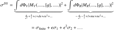
σDS =
Z
dΦV|MV(...,[g], ...)|2
| {z } a
✏2+ b
✏+c+d✏+e✏2+...
+
Z
dΦR|MR(....,[g], ....)|2
| {z } −a
✏2− b
✏+l+m✏+n✏2+...
=σfinite+✏σ1+✏2σ2+. . . (5)
where the scheme independent terms cancel and the analytic part of the expansion is scheme independent except for the first term. Regardless on the scheme the physical cross section should be obtained as
σ=lim
✏!0σ DS =σ
finite (6)
if the adopted regularization scheme is compatible with the unitarity of the theory,
mean-ing with the statement of the the optical theorem. The purelyd-dimensional treatment of
all objects, the so called conventional (or naive) dimensional regularization is conceptually
simpler, but it breaks supersymmetry and it gives ambiguities like Tr(γ5γµγ⌫γ⇢γ⌧) with chiral
symmetries, but it is unitarity compatible [3]. However for the modern techniques of gen-eralized unitarity [4] of the integrand reconstruction by gluing tree level helicity amplitudes, a four dimensional approach in general considerably simplifies the computations. In those cases the 4-dimensional treatment of the gluons is better compatible with supersymmetry and it is more amenable to helicity methods, where we glue amplitudes like the one coming from the Parke-Taylor [5] formula for Maximally Helicity Violating amplitudes
AMHV(1+, ...,i−, ...,j−, ...n+)=i(−g)n−2 <i j> 4
<12><23> ... <n1> (7)
written here in terms of the helicity spinors, pedagogically introduced in [6]. The previous
considerations imply the need for a dimensional reduction of theddimensional vector field
to a four dimensional one together with a dimensional regularization of the loop integrals.
2 Variants of the dimensional regularization
There is an elegant way to unify essentially all common variants of dimensional regular-ization in a single framework, where all definitions can easily be formulated and where the
di↵erences and relations between the schemes become transparent [7]. Such a framework is
based on the introduction of three vector spaces: the original four dimensional space (4S)
and the infinite dimensional vector spaces, intrinsic in every dimensional scheme to provide the regularization of theories formulated in an arbitrary number of dimensions [8]. The space
(4S) has metric tensorgµ⌫[4], then we have the “quasi-d-dimensional" space (QS[d]) with metric
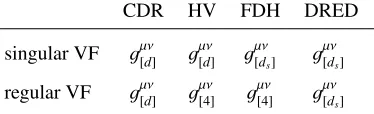
CDR HV FDH DRED
singular VF gµ⌫[d] gµ⌫[d] gµ⌫[ds] gµ⌫[ds]
regular VF gµ⌫[d] gµ⌫[4] gµ⌫[4] gµ⌫[ds]
Table 1.Treatment of vector fields in the four di↵erent regularization schemes, i.e. prescription which
metric tensor has to be used in propagator numerators and polarization sums. The quantitydsis
usually taken to be 4.
tensorgµ⌫[d], the “quasi-ds-dimensional" space (QS[ds]) with metric tensorg
µ⌫
[ds]. The
“quasi-dimensionalities" of those infinite dimensional spaces are related by the following relations between the complex numbers:
ds=d+n✏ =4−2✏+n✏, (8)
implying the following formal direct sum and inclusions
QS[ds] =QS[d]⊕QS[n✏] S4⇢QS[d] ⇢QS[ds]. (9)
Indeed since only gluons that appear inside a divergent loop or phase space integral need to be regularized, those are called “singular" gluons and all the others are called “regular". Based on that distinction the following variants of dimensional regularization and dimen-sional reduction are introduced. CDR (“Conventional dimendimen-sional regularization") in which
singular and regular gluons (and other vector fields) are all treated as quasi-d−dimensional.
HV (“ ’t Hooft Veltman") in which singular gluons are treated as quasi-d−dimensional but
the regular ones are treated as 4−dimensional. For the dimensional reduction we have DRED
(“original/old dimensional reduction"), where regular and singular gluons are all treated as
quasi-ds-dimensional, and FDH (“four-dimensional helicity scheme") so that singular gluons
are treated as quasi-ds-dimensional but external ones are treated as 4-dimensional.
The treatment of vector fields in the four di↵erent regularization schemes and the
corre-sponding prescriptions on which metric tensor has to be used in propagator numerators and vectors polarization sums are summarized in the table 1.
In order to use FDH and DRED, the variants based on the dimensional reduction, the
crucial step is to split quasi-ds-dimensional gluons intod-component gauge fields andn✏ !
2✏scalar fields, so called✏-scalars, as from the decomposition of the metric tensor
(g[ds]) µ⌫ =(g
[d])µ⌫+(g[n✏])
µ⌫ (10)
with the algebra
gµ⌫[ds](g[d])⌫⇢=(g[d])µ⇢, g µ⌫
[ds](g[n✏])⌫⇢=(g[n✏])
µ ⇢, g
µ⌫
[d](g[n✏])⌫⇢=0, (g[n✏])⌫⇢g
⇢µ
[4]=0. (11)
Since new degrees of freedom enter in the game, the independence of the gauge boson
man-ifest in the couplings of the ✏-scalars resulting in di↵erent renormalization constants and
β-functions. In QED the gauge couplingeand the evanescent couplingeerenormalize di↵
er-ently being not protected by the Lorentz and the gauge invariance onQS[d]
βe=µ2DS d
dµ2DS
✓ e
4⇡
◆2
= 4
3 ✓ e
4⇡
◆4
poles. Actually the integral (1), combined with other UV and IR divergent terms, is usually defined [2] so that to cancel those divergences and not to bring contributions to the finite part. Consider the physical cross section at the Next-to-Leading Order which receives by the Kinoshita- Lee- Nauenberg theorem the real and virtual contributions
σ=σV+σR =
Z
dΦV|MV|2+
Z
dΦR|MR|2, (4)
identified by the corresponding amplitudes MR andMV. A complete dimensional scheme
(DS), meaning a complete procedure to make the analytical dimensional continuation in the
dynamics of the theory is reflected at the level of the Feynman integrals by the way of treating
the gauge boson metric, generically indicated in the following byg:
σDS =
Z
dΦV|MV(...,[g], ...)|2
| {z } a
✏2+ b
✏+c+d✏+e✏2+...
+
Z
dΦR|MR(....,[g], ....)|2
| {z } −a
✏2− b
✏+l+m✏+n✏2+...
=σfinite+✏σ1+✏2σ2+. . . (5)
where the scheme independent terms cancel and the analytic part of the expansion is scheme independent except for the first term. Regardless on the scheme the physical cross section should be obtained as
σ=lim
✏!0σ DS =σ
finite (6)
if the adopted regularization scheme is compatible with the unitarity of the theory,
mean-ing with the statement of the the optical theorem. The purelyd-dimensional treatment of
all objects, the so called conventional (or naive) dimensional regularization is conceptually
simpler, but it breaks supersymmetry and it gives ambiguities like Tr(γ5γµγ⌫γ⇢γ⌧) with chiral
symmetries, but it is unitarity compatible [3]. However for the modern techniques of gen-eralized unitarity [4] of the integrand reconstruction by gluing tree level helicity amplitudes, a four dimensional approach in general considerably simplifies the computations. In those cases the 4-dimensional treatment of the gluons is better compatible with supersymmetry and it is more amenable to helicity methods, where we glue amplitudes like the one coming from the Parke-Taylor [5] formula for Maximally Helicity Violating amplitudes
AMHV(1+, ...,i−, ...,j−, ...n+)=i(−g)n−2 <i j> 4
<12><23> ... <n1> (7)
written here in terms of the helicity spinors, pedagogically introduced in [6]. The previous
considerations imply the need for a dimensional reduction of theddimensional vector field
to a four dimensional one together with a dimensional regularization of the loop integrals.
2 Variants of the dimensional regularization
There is an elegant way to unify essentially all common variants of dimensional regular-ization in a single framework, where all definitions can easily be formulated and where the
di↵erences and relations between the schemes become transparent [7]. Such a framework is
based on the introduction of three vector spaces: the original four dimensional space (4S)
and the infinite dimensional vector spaces, intrinsic in every dimensional scheme to provide the regularization of theories formulated in an arbitrary number of dimensions [8]. The space
(4S) has metric tensorgµ⌫[4], then we have the “quasi-d-dimensional" space (QS[d]) with metric
CDR HV FDH DRED
singular VF gµ⌫[d] gµ⌫[d] gµ⌫[ds] gµ⌫[ds]
regular VF gµ⌫[d] gµ⌫[4] gµ⌫[4] gµ⌫[ds]
Table 1.Treatment of vector fields in the four di↵erent regularization schemes, i.e. prescription which
metric tensor has to be used in propagator numerators and polarization sums. The quantitydsis
usually taken to be 4.
tensorgµ⌫[d], the “quasi-ds-dimensional" space (QS[ds]) with metric tensorg
µ⌫
[ds]. The
“quasi-dimensionalities" of those infinite dimensional spaces are related by the following relations between the complex numbers:
ds=d+n✏=4−2✏+n✏, (8)
implying the following formal direct sum and inclusions
QS[ds]=QS[d]⊕QS[n✏] S4⇢QS[d]⇢QS[ds]. (9)
Indeed since only gluons that appear inside a divergent loop or phase space integral need to be regularized, those are called “singular" gluons and all the others are called “regular". Based on that distinction the following variants of dimensional regularization and dimen-sional reduction are introduced. CDR (“Conventional dimendimen-sional regularization") in which
singular and regular gluons (and other vector fields) are all treated as quasi-d−dimensional.
HV (“ ’t Hooft Veltman") in which singular gluons are treated as quasi-d−dimensional but
the regular ones are treated as 4−dimensional. For the dimensional reduction we have DRED
(“original/old dimensional reduction"), where regular and singular gluons are all treated as
quasi-ds-dimensional, and FDH (“four-dimensional helicity scheme") so that singular gluons
are treated as quasi-ds-dimensional but external ones are treated as 4-dimensional.
The treatment of vector fields in the four di↵erent regularization schemes and the
corre-sponding prescriptions on which metric tensor has to be used in propagator numerators and vectors polarization sums are summarized in the table 1.
In order to use FDH and DRED, the variants based on the dimensional reduction, the
crucial step is to split quasi-ds-dimensional gluons intod-component gauge fields andn✏ !
2✏scalar fields, so called✏-scalars, as from the decomposition of the metric tensor
(g[ds]) µ⌫ =(g
[d])µ⌫+(g[n✏])
µ⌫ (10)
with the algebra
gµ⌫[ds](g[d])⌫⇢=(g[d])µ⇢, g µ⌫
[ds](g[n✏])⌫⇢=(g[n✏])
µ ⇢, g
µ⌫
[d](g[n✏])⌫⇢ =0, (g[n✏])⌫⇢g
⇢µ
[4]=0. (11)
Since new degrees of freedom enter in the game, the independence of the gauge boson
man-ifest in the couplings of the ✏-scalars resulting in di↵erent renormalization constants and
β-functions. In QED the gauge couplingeand the evanescent couplingeerenormalize di↵
er-ently being not protected by the Lorentz and the gauge invariance onQS[d]
βe=µ2DS d
dµ2DS
✓ e
4⇡
◆2
= 4
3 ✓e
4⇡
◆4
βee =µ2DS
d dµ2DS
✓ee
4⇡
◆2
=6
✓ e
4⇡
◆4 −6✓ e
4⇡
◆2✓ee
4⇡
◆2
+. . . (13)
Even by imposing the renormalization conditione =eethe flows of the two couplings are
di↵erent [7].
3 FDF:Four dimensional formulation of the FDH scheme
FDF is a novel regularization approach that was introduced to reproduce FDH results at the one-loop level [9]. Starting from unregularized expressions in one loop diagram the loop
momenta are shifted as /`[d] ! /`[4]+iµγ5 before any other algebraic manipulation is
per-formed. The matrixγ5provides the chirality in four dimensions. The scaleµcorresponds to
the otherd−4 dimensional components of the loop momentum and serves as regulator for
the in general divergent quasi-ddimensional loop momentum in the integral. By definition,
odd powers ofµare set to zero, resulting in the useful relation
/`[d]/`[d]=`2[d]=`[4]2 −µ2. (14)
One main advantage with FDF approach is that the Lorentz algebra is realized in strictly
four dimensions. By construction the treatment ofγ5in FDF unifies those of
Breitenlohner-Maison and the anti-commuting chiral prescriptions like in the ’t Hooft-Veltman [10]. Due to the previously declared shift the fermionic cutted lines in the diagrams obey to a
generalized Dirac equation �
/`[4]+iµγ5+m�u(`)=0. (15)
By expressing the four momenta in terms of the massless four-momenta`[
[4] andq`[4] the
spinors generalized solutions are
u+(`)=���`[[4]E+ m−iµ
[`[ [4],q`[4]]
��
�q`[4]⇤ u−(`)=���`[[4]
i
+ m+iµ
< `[
[4],q`[4]>
��
�q`[4]↵ (16)
with the usual notation of the helicity spinors. In [9] it is possible to find the wave functions for the cut gluonic and scalar lines for the consequent dimensional reduction involved in this procedure.
At one loop it is known the decomposition of any scattering amplitude in terms of a basis of master scalar integrals á la Passarino-Veltman [11]. By FDF we have a tool to add ad-ditional basis integrals at one loop consisting, in the case of having massless internal lines,
into two sets of additional boxesI4[(µ2)2],I4[µ2], additional trianglesI3[µ2] and additional
bubblesI2[µ2], with the notations of having insertions ofµ2in the numerators of those
addi-tional master integrals. The decomposition of that amplitude in this basis involve coefficients
of the additional integrals that are independent of the dimensional regulator, therefore those
coefficients can be computed by integration contours using the methods of algebraic
geome-try [12]. The amplitude in now expressed in terms of larger set of integrals that in principle they could be evaluated as they are, however it is usually easier to evaluate them in terms of
standard integrals.When we do that the dependence on the✏regulator reappears, in fact at
one loop the conversion to the standard integrals amounts to a shift of the dimensionality, one has dimension shift identities like [15]
I4[(µ2)2]=−✏(1−✏)16⇡2I48−2✏[1]. (17)
For a box integral we have now five degrees of freedom instead of four. The so called quadruple cut [13], which is the modern procedure of extracting the leading singularity of
one-loop amplitudes (contrast it to [14]) and which allows the calculation of the box
co-efficients in the scattering amplitudes, is in terms of this basis a one-dimensional surface
µ-dependent more than a single point in the space of the momenta. However after gluing the
corresponding amplitudes the box coefficients of the two integrals in the extended basis are
still found by collecting in the numerators respectively the coefficients of the monomial (µ2)2
andµ2. In fact by removing factors with✏exponents from the measured4−2✏k=d4k d−2✏k
and multiplying by a weight function ofµ2to isolate di↵erent integrals we find in terms of
the block amplitudes the coefficients of the extra basis integrals as
ci=
I dµ2
µ2 A 1
tree(µ2)A2tree(µ2)Atree3 (µ2)A4tree(µ2), (18)
with a final result compatible with [16].
4 Foundational work to perform two loops reductions in FDF
First of all we need a basis, this has been provided in pure 4 dimensions for planar diagrams
in [17]. The notations for the double box P⇤
n1,n2, refer ton1 lines on the right andn2 lines
on the left of the double box. In this basis we have two integrals for massless, one-mass,
diagonal-two mass double box P⇤
2,2. Three integrals for short side two mass, three-mass
double box. Four integrals for four masses double box. One integral for massless pentabox P⇤
3,2. A pure four dimensional basis is reduced to this with master integrals containing up
to height propagators. More complicated integrals can be reduced to them up to✏-terms.
The new feature compared with the one-loop case is the presence of irreducible numerators even when it is simply involved the scalar product of a loop momentum with an external leg, meaning that they cannot be written as linear combination of the denominators propagators and external invariants.
To perform the reduction to the previous basis at two loops the tensor reduction is still
necessary and useful but it is not sufficient, because some additional technology is needed in
order to take care of the irreducible invariants and their powers. That technology is based on the so-called integration by part identities (IBP) [18]. This technology is based on an axiom of dimensional regularization that the integral of a total divergence is zero, because there are no boundary terms
0=
Z dd`
1dd`2 @ @`µ1
vµ
Denominator (19)
this gives linear relations between integrals that can be solved in terms of the independent master integrals. In the notation of the previous equation a so called IBP generating vector is included which takes care of the fact that no doubled propagators are generated in the IBP, this simplifies the solution of the system of the IBP. By identifying the IBP generating vectors would provide a quicker approach to solve the system for generating master integrals [17]. By
the definition of the vectorsvµ, they are algebraic geometric objects arising from appropriate
polynomial divisions, their algebraically geometric properties as well as their connection to
the di↵erent topologies of the basis need still to be completely studied. In the aim of finding
a two-loop basis with coefficients still independent of the regularization parameter, the IBP
arise a kind of line-one problem:
@ @`1µ
`µ1
Denominator=
4−2✏
βee =µ2DS
d dµ2DS
✓ee
4⇡
◆2
=6
✓e
4⇡
◆4 −6✓ e
4⇡
◆2✓ee
4⇡
◆2
+. . . (13)
Even by imposing the renormalization conditione = eethe flows of the two couplings are
di↵erent [7].
3 FDF:Four dimensional formulation of the FDH scheme
FDF is a novel regularization approach that was introduced to reproduce FDH results at the one-loop level [9]. Starting from unregularized expressions in one loop diagram the loop
momenta are shifted as /`[d] ! /`[4]+iµγ5 before any other algebraic manipulation is
per-formed. The matrixγ5provides the chirality in four dimensions. The scaleµcorresponds to
the otherd−4 dimensional components of the loop momentum and serves as regulator for
the in general divergent quasi-ddimensional loop momentum in the integral. By definition,
odd powers ofµare set to zero, resulting in the useful relation
/`[d]/`[d]=`2[d] =`2[4]−µ2. (14)
One main advantage with FDF approach is that the Lorentz algebra is realized in strictly
four dimensions. By construction the treatment ofγ5in FDF unifies those of
Breitenlohner-Maison and the anti-commuting chiral prescriptions like in the ’t Hooft-Veltman [10]. Due to the previously declared shift the fermionic cutted lines in the diagrams obey to a
generalized Dirac equation �
/`[4]+iµγ5+m�u(`)=0. (15)
By expressing the four momenta in terms of the massless four-momenta `[
[4] andq`[4] the
spinors generalized solutions are
u+(`)=���`[[4]E+ m−iµ
[`[ [4],q`[4]]
��
�q`[4]⇤ u−(`)=���`[[4]
i
+ m+iµ
< `[
[4],q`[4]>
��
�q`[4]↵ (16)
with the usual notation of the helicity spinors. In [9] it is possible to find the wave functions for the cut gluonic and scalar lines for the consequent dimensional reduction involved in this procedure.
At one loop it is known the decomposition of any scattering amplitude in terms of a basis of master scalar integrals á la Passarino-Veltman [11]. By FDF we have a tool to add ad-ditional basis integrals at one loop consisting, in the case of having massless internal lines,
into two sets of additional boxesI4[(µ2)2],I4[µ2], additional trianglesI3[µ2] and additional
bubblesI2[µ2], with the notations of having insertions ofµ2in the numerators of those
addi-tional master integrals. The decomposition of that amplitude in this basis involve coefficients
of the additional integrals that are independent of the dimensional regulator, therefore those
coefficients can be computed by integration contours using the methods of algebraic
geome-try [12]. The amplitude in now expressed in terms of larger set of integrals that in principle they could be evaluated as they are, however it is usually easier to evaluate them in terms of
standard integrals.When we do that the dependence on the✏ regulator reappears, in fact at
one loop the conversion to the standard integrals amounts to a shift of the dimensionality, one has dimension shift identities like [15]
I4[(µ2)2]=−✏(1−✏)16⇡2I48−2✏[1]. (17)
For a box integral we have now five degrees of freedom instead of four. The so called quadruple cut [13], which is the modern procedure of extracting the leading singularity of
one-loop amplitudes (contrast it to [14]) and which allows the calculation of the box
co-efficients in the scattering amplitudes, is in terms of this basis a one-dimensional surface
µ-dependent more than a single point in the space of the momenta. However after gluing the
corresponding amplitudes the box coefficients of the two integrals in the extended basis are
still found by collecting in the numerators respectively the coefficients of the monomial (µ2)2
andµ2. In fact by removing factors with✏ exponents from the measured4−2✏k= d4k d−2✏k
and multiplying by a weight function ofµ2to isolate di↵erent integrals we find in terms of
the block amplitudes the coefficients of the extra basis integrals as
ci=
I dµ2
µ2 A 1
tree(µ2)A2tree(µ2)Atree3 (µ2)A4tree(µ2), (18)
with a final result compatible with [16].
4 Foundational work to perform two loops reductions in FDF
First of all we need a basis, this has been provided in pure 4 dimensions for planar diagrams
in [17]. The notations for the double box P⇤
n1,n2, refer ton1 lines on the right andn2 lines
on the left of the double box. In this basis we have two integrals for massless, one-mass,
diagonal-two mass double box P⇤
2,2. Three integrals for short side two mass, three-mass
double box. Four integrals for four masses double box. One integral for massless pentabox P⇤
3,2. A pure four dimensional basis is reduced to this with master integrals containing up
to height propagators. More complicated integrals can be reduced to them up to✏-terms.
The new feature compared with the one-loop case is the presence of irreducible numerators even when it is simply involved the scalar product of a loop momentum with an external leg, meaning that they cannot be written as linear combination of the denominators propagators and external invariants.
To perform the reduction to the previous basis at two loops the tensor reduction is still
necessary and useful but it is not sufficient, because some additional technology is needed in
order to take care of the irreducible invariants and their powers. That technology is based on the so-called integration by part identities (IBP) [18]. This technology is based on an axiom of dimensional regularization that the integral of a total divergence is zero, because there are no boundary terms
0=
Z dd`
1dd`2 @ @`1µ
vµ
Denominator (19)
this gives linear relations between integrals that can be solved in terms of the independent master integrals. In the notation of the previous equation a so called IBP generating vector is included which takes care of the fact that no doubled propagators are generated in the IBP, this simplifies the solution of the system of the IBP. By identifying the IBP generating vectors would provide a quicker approach to solve the system for generating master integrals [17]. By
the definition of the vectorsvµ, they are algebraic geometric objects arising from appropriate
polynomial divisions, their algebraically geometric properties as well as their connection to
the di↵erent topologies of the basis need still to be completely studied. In the aim of finding
a two-loop basis with coefficients still independent of the regularization parameter, the IBP
arise a kind of line-one problem:
@ @`µ1
`µ1
Denominator =
4−2✏
consequently✏ seems to be intrinsic to these reductions bringing to a decomposition of the
type
Ampl= X
j2Basis
cj(✏)Intj (21)
as for instance in the one-loop bubble by Passarino-Veltman reduction
Bµ⌫(k2)= 2−✏
4(3−2✏)B0(k2)k
µ [4]k[4]⌫ −
1
4(3−2✏)B0(k2)g
µ⌫
[4]. (22)
This is a problem in view of implementing the 4−2✏dimensional generalized unitarity
pro-gram, for which it is desired a basis with coefficients which are✏independent. The
regular-izer✏is indeed something deeply related to the integration on the real slice. By the methods
of generalized unitarity we want indeed to perform integration on contours in the complex
plane to isolate the appropriate residues, clearly we cannot have a basis which is✏
depen-dent, because the✏dependence is obtained from integration on the real slice. The conjecture
considered here [19] is that again at two-loop there is an augmented basis, which now will
depend onµ21,µ22,µ1·µ2. The tree amplitudes to be glued in the integrand reconstruction
indeed come from the six dimensional extension of the theory [20]. By FDF we can recon-struct the total dependence of the two-loop integrands in terms of the extra dimensions using an appropriate modifications of FDF in terms of six dimensional ingredients [21]. However the recursive construction of the Dirac gamma matrices in higher dimensions is based on an operation of tensor product having the structure with four dimensional ingredients as seed of generation of the Dirac representation of the Lorentz group in higher dimensions [22]. In this sense FDF seems to be a basic block so that modulo multiplication with appropriate sigma Pauli matrices, the FDF results for the tree amplitudes computations [9] in the generalized unitarity procedure can be exported to two loops.
The way proposed here to reach such an augmented basis is thorough four-dimensional IBP
0=
Z dd`
1dd`2 @ @`µ[4]i
vµ[4]
Denominator (23)
The involved IBP generating vectorsvµ[4] will be dependent on theµ21,µ22,µ1·µ2 and even
for simple integrals like the double box they have not been computed yet, however it is
ex-pected that their algebraic geometry is very di↵erent form the ones coming from the IBP ind
dimensions.
The last ingredient that we need is how to convert back to standard integrals. We have
the additional componentsµi inside integrand we want to go back to recover✏. There are
basically two techniques to be combined:
• take a Gram determinants [G({pi},{qi})] =deti,j(pi·qj), do Feynman parametrization to
get relations like this
P⇤,⇤
2,2[(µ21)2]=−
✏(1−✏)
(3−2✏)(1−2✏)G2
124
P⇤,⇤
2,2[G2(`1,1,2,4)] (24)
where together with a rational function of✏there is the dependence onG2
124, an invariant
of the external momenta;
• perform standard (d-dimensional) IBPs withµifactors and irreducible products inserted in
the numerators
0=
Z dd`
1dd`2 @ @`µi[d]
{1, µ21, ...}(irreducible)jvµ [4]
Denominator . (25)
5 Conclusions
Alternative dimensional regularization schemes are available for higher order computations in perturbative gauge theories. However there is not a wide use of them. It is needed to
pro-vide more practical examples to show the efficiency of those schemes.The four dimensional
formulation (FDF) of the four dimensional helicity scheme (FDH) is a proposal to get the cut constructible and the rational part of one-loop amplitudes by just four dimensional cuts. FDF
is efficient to find contributions of evanescent operators in perturbative computations. The
foundations ford-dimensional unitarity within FDF at two loops have been discussed.
References
[1] G. Leibbrandt, Rev.Mod.Phys.47, 849 (1975) .
[2] D. Bardin, G.Passarino,The Standard Model in the making( Claredon Press, New York,
1999 ) pp. 166-169.
[3] G. ’t Hooft, M.J.G. Veltman, Nucl.Phys. B50, 318 (1972).
[4] Z. Bern, L.J. Dixon, D.A. Kosower, Annals Phys.322, 1587 (2007).
[5] I suggest for a review: T.R. Taylor, Phys.Rept.691, 1 (2017).
[6] M.E. Peskin, arXiv:1101.2414 [hep-ph].
[7] C. Gnendinger et al., Eur. Phys. J. C77, 471 (2017).
[8] J.C. Collins,Renormalization(Cambridge University Press, Cambridge, 1984) pp.
62-87.
[9] A.R. Fazio, P. Mastrolia, E. Mirabella, W.J. Torres Bobadilla, Eur. Phys. J. C74, 3197
(2014).
[10] C. Gnendiger, A. Signer, Phys.Rev. D97, 096006 (2018).
[11] G. Passarino, M. Veltman, Nucl. Phys. B160151 (1979).
[12] D. A. Kosower, K. J. Larsen, Phys.Rev. D85, 045017 (2012).
[13] R. Britto, F. Cachazo, B. Feng, Nucl.Phys. B725275 (2005).
[14] Eden, Landsho↵, Olive, PolkinghorneThe analytic S-matrix(Cambridge at University
press, Cambrdge, 1966) chap. 2.
[15] Z. Bern, A.G. Morgan, Nucl.Phys. B467, 479 (1996).
[16] S.D. Badger, JHEP0901, 049 (2009).
[17] J.Gluza, K. Kajida, D. A. Kosower , Phys.Rev. D83, 045012 (2011).
[18] For a review: V.A. Smirnov,Analytic tools for Feynman integrals(Springer, London,
2012 ) pp. 127-154.
[19] D.A. Kosower,Maximal Unitarity and Algebraic Geometry, talk given at IAS focused
program in Scattering Amplitudes in Hong Kong, November 2014.
[20] S. Badger, C. Bronnum-Hansen, H. Bayu Hartanto, T. Peraro, Phys.Rev.Lett.120no.9,
092001 (2018).
[21] A.R. Fazio, P. Mastrolia, W.J. Torres,to appear.
[22] P. van Nieuwenhuizen,Six Lectures at the Trieste 1981 Summer School on Supergravity,
consequently✏ seems to be intrinsic to these reductions bringing to a decomposition of the
type
Ampl= X
j2Basis
cj(✏)Intj (21)
as for instance in the one-loop bubble by Passarino-Veltman reduction
Bµ⌫(k2)= 2−✏
4(3−2✏)B0(k2)k
µ [4]k⌫[4]−
1
4(3−2✏)B0(k2)g
µ⌫
[4]. (22)
This is a problem in view of implementing the 4−2✏dimensional generalized unitarity
pro-gram, for which it is desired a basis with coefficients which are✏independent. The
regular-izer✏is indeed something deeply related to the integration on the real slice. By the methods
of generalized unitarity we want indeed to perform integration on contours in the complex
plane to isolate the appropriate residues, clearly we cannot have a basis which is✏
depen-dent, because the✏dependence is obtained from integration on the real slice. The conjecture
considered here [19] is that again at two-loop there is an augmented basis, which now will
depend onµ21,µ22,µ1·µ2. The tree amplitudes to be glued in the integrand reconstruction
indeed come from the six dimensional extension of the theory [20]. By FDF we can recon-struct the total dependence of the two-loop integrands in terms of the extra dimensions using an appropriate modifications of FDF in terms of six dimensional ingredients [21]. However the recursive construction of the Dirac gamma matrices in higher dimensions is based on an operation of tensor product having the structure with four dimensional ingredients as seed of generation of the Dirac representation of the Lorentz group in higher dimensions [22]. In this sense FDF seems to be a basic block so that modulo multiplication with appropriate sigma Pauli matrices, the FDF results for the tree amplitudes computations [9] in the generalized unitarity procedure can be exported to two loops.
The way proposed here to reach such an augmented basis is thorough four-dimensional IBP
0=
Z dd`
1dd`2 @ @`µ[4]i
vµ[4]
Denominator (23)
The involved IBP generating vectorsvµ[4] will be dependent on theµ21,µ22,µ1·µ2 and even
for simple integrals like the double box they have not been computed yet, however it is
ex-pected that their algebraic geometry is very di↵erent form the ones coming from the IBP ind
dimensions.
The last ingredient that we need is how to convert back to standard integrals. We have
the additional componentsµi inside integrand we want to go back to recover✏. There are
basically two techniques to be combined:
• take a Gram determinants [G({pi},{qi})] = deti,j(pi·qj), do Feynman parametrization to
get relations like this
P⇤,⇤
2,2[(µ21)2]=−
✏(1−✏)
(3−2✏)(1−2✏)G2
124
P⇤,⇤
2,2[G2(`1,1,2,4)] (24)
where together with a rational function of✏ there is the dependence onG2
124, an invariant
of the external momenta;
• perform standard (d-dimensional) IBPs withµifactors and irreducible products inserted in
the numerators
0=
Z dd`
1dd`2 @ @`µi[d]
{1, µ21, ...}(irreducible)jvµ [4]
Denominator . (25)
5 Conclusions
Alternative dimensional regularization schemes are available for higher order computations in perturbative gauge theories. However there is not a wide use of them. It is needed to
pro-vide more practical examples to show the efficiency of those schemes.The four dimensional
formulation (FDF) of the four dimensional helicity scheme (FDH) is a proposal to get the cut constructible and the rational part of one-loop amplitudes by just four dimensional cuts. FDF
is efficient to find contributions of evanescent operators in perturbative computations. The
foundations ford-dimensional unitarity within FDF at two loops have been discussed.
References
[1] G. Leibbrandt, Rev.Mod.Phys.47, 849 (1975) .
[2] D. Bardin, G.Passarino,The Standard Model in the making( Claredon Press, New York,
1999 ) pp. 166-169.
[3] G. ’t Hooft, M.J.G. Veltman, Nucl.Phys. B50, 318 (1972).
[4] Z. Bern, L.J. Dixon, D.A. Kosower, Annals Phys.322, 1587 (2007).
[5] I suggest for a review: T.R. Taylor, Phys.Rept.691, 1 (2017).
[6] M.E. Peskin, arXiv:1101.2414 [hep-ph].
[7] C. Gnendinger et al., Eur. Phys. J. C77, 471 (2017).
[8] J.C. Collins,Renormalization(Cambridge University Press, Cambridge, 1984) pp.
62-87.
[9] A.R. Fazio, P. Mastrolia, E. Mirabella, W.J. Torres Bobadilla, Eur. Phys. J. C74, 3197
(2014).
[10] C. Gnendiger, A. Signer, Phys.Rev. D97, 096006 (2018).
[11] G. Passarino, M. Veltman, Nucl. Phys. B160151 (1979).
[12] D. A. Kosower, K. J. Larsen, Phys.Rev. D85, 045017 (2012).
[13] R. Britto, F. Cachazo, B. Feng, Nucl.Phys. B725275 (2005).
[14] Eden, Landsho↵, Olive, PolkinghorneThe analytic S-matrix(Cambridge at University
press, Cambrdge, 1966) chap. 2.
[15] Z. Bern, A.G. Morgan, Nucl.Phys. B467, 479 (1996).
[16] S.D. Badger, JHEP0901, 049 (2009).
[17] J.Gluza, K. Kajida, D. A. Kosower , Phys.Rev. D83, 045012 (2011).
[18] For a review: V.A. Smirnov,Analytic tools for Feynman integrals(Springer, London,
2012 ) pp. 127-154.
[19] D.A. Kosower,Maximal Unitarity and Algebraic Geometry, talk given at IAS focused
program in Scattering Amplitudes in Hong Kong, November 2014.
[20] S. Badger, C. Bronnum-Hansen, H. Bayu Hartanto, T. Peraro, Phys.Rev.Lett.120no.9,
092001 (2018).
[21] A.R. Fazio, P. Mastrolia, W.J. Torres,to appear.
[22] P. van Nieuwenhuizen,Six Lectures at the Trieste 1981 Summer School on Supergravity,