The Coalescent Process With Selfing

Copyright 0 1997 by the Genetics Society of America

The Coalescent Process

With Selfing

Magnus

Nordborg” and Peter Donnelly’

*Department of Ecology and Evolution, University of Chicago, Chicago, Illinois 60637-1573 and tDepartment of Statistics, University of Oxford, Oxford OX1 3TG, United Kingdom

Manuscript received August 15, 1996 Accepted for publication March 28, 1997

ABSTRACT

A method for estimating the selfing rate using DNA sequence data was recently proposed by Milligan. Unfortunately, a number of errors make interpretation of his results problematic. In the present paper we first show how the usual coalescent process can be adapted to models that include selfing, and then use this result to find moment estimators as well as the likelihood surface for the selfing rate, s, and the scaled mutation rate, 0. We conclude that, regardless of the method used, large sample sizes are necessary to estimate s with any degree of certainty, and that the estimate is always highly sensitive to recent changes in the true value.

T

HERE is long-standing interest in estimating the degree of self-fertilization, or selfing, in partially selfing populations. Several methods have been sug- gested, most of them based on allozyme frequency data (BROWN 1990). Recently, MILLIGAN ( 1996) suggested a method using DNA sequence data based on the differ- ence in coalescence time for alleles sampled within and between an individual.

In this article, we first show in general how the stan- dard neutral coalescent process can be used for models with partial selfing. We use this result to derive alterna- tives to MILLIGAN’S estimator and to compare the prop- erties of the estimators. Finally, we discuss the use- fulness of DNA data for estimating the selfing rate.

THE COALESCENT PROCESS WITH

PARTIAL SELFING

Consider a Wright-Fisher model of N diploid her- maphrodites, with Nvery large. Define the selfing rate s as the fraction of offspring that is produced by self- fertilization. The remaining fraction 1 - s is produced via random mating. For a single locus with two alleles, it is easy to show that the genotypic proportions quickly converge to

p‘

+

pqF,

2pq(

1 -

F)

, and

q‘

+

pqF, where

F =

- S

2 - s

is the equilibrium inbreeding coefficient ( HALDANE

1924).

Now consider the dynamics of a single neutral allele when N is finite. Under the assumption that s % 1

/

N , it has been argued, using the diffusion approximation, that the theory for random mating populations holds with variance (and inbreeding) effective population size of

Curresponding author: Magnus Nordborg, Department of Ecology

and Evolution, University of Chicago, 1101 E. 57th St., Chicago, IL 60637-1573. E-mail: [email protected]

Genetirs 1 4 6 1185-1195 (July, 1997)

1 2 - s

N, = -

l + F N =

-

2

N

( LI 1955; WRIGHT 1969; POLM 1987).

We will describe the analogous result for the standard n-coalescent ( K ~ N G M A N 1982a,c; TAV& 1984). More precisely, we will demonstrate that, apart from its initial behavior, the coalescent with partial selfing is identical to the coalescent for random mating if time is rescaled by a factor corresponding to the variance effective pop- ulation size ( 2 ) . This similarity should not be unex- pected given the close correspondence between vari- ance effective population size and the time scale of the coalescent ( K ~ N G M A N 1982b).

Take the case of two alleles first (in the context of the coalescent, we will use “allele” to denote a region of DNA within which recombination can be ignored). With random mating, we simply trace their ancestry until a single allele that is their common ancestor is found. Going backward in time, we have a Markov pro- cess with two states: two alleles, or a single common ancestral allele (this state is of course absorbing). With selfing the same process has three states: two alleles in distinct individuals, two distinct alleles in the same individ- ual, and a single common ancestral allele.

It is easy to see that the transition matrix (with the states in the order described) for this process is

1 1

N 2N 2N

-

P =

( 1 -s)

+

(I(;)

;+(I(;)

;+

(I(;)

L

0 0

1186 M. Nordborg and P. Donnelly

distinct individuals for a random amount of time that is geometrically distributed with expectation N. When the process leaves this state (because the two alleles find themselves in the same ancestral individual), the common ancestral allele is found, and thus the process jumps to the third state, with probability else the process jumps to its second state: two distinct alleles in the same individual. When the process is in its second state, it follows from the transition matrix ( 3 ) that it remains there for a random number of generations that is geometrically distributed with expectation

s/

( 2 - s )

+

O ( 1

/

N)

.

When it leaves the second state, a common ancestor will be found, and so the process will jump to its third state, with probability

otherwise it returns its first state: two alleles in distinct individuals.

In summary, the process remains in the first state for an amount of time that is geometrically distributed with expectation of O ( N ) , after which either a common ancestor is found with probability 1/2 or the process jumps to the second state. The process remains in the second state for an amount of time that is geometrically distributed with expectation of O( 1 ) , after which a common ancestor is found with approximate probabil- ity s/ ( 2 - s) , or else the process returns to the first state.

Recall that in the coalescent, time is measured in units of O(

N)

generations. With this time-scaling, any time spent in the second state is negligible. Thus in the coalescent approximation to models with selfing, the second state becomes instantaneous. If the process starts in this state, it will leave it instantaneously for either the first or the third state, with respective proba- bilities 1 - s/ ( 2 - s) and s/ ( 2 - s)

.

If the process starts in the first state, we will never “see” any time spent in the second state. A proportion 1 - s/

( 2

- s) of transitions to the second state will instantaneously return to the first state, while the remaining proportion

s/ ( 2 - s) will move instantaneously to the third state. Thus, with time measured in units of N generations, the process moves from the first state to the third state with rate

Alternatively, if time is measured in units of ( 2 - s) N generations (that is, 2N,, where Ne is given by Equation

2 ) , the process waits in the first state for an exponen- tially distributed amount of time with mean one before coalescing ( i e . , moving to the third state)

.

If the two alleles of interest are sampled from the same individual, the process starts in the second state, but moves instan- taneously to either the first or third state, with the prob- abilities given above. Thus, except for this initial behav-

ior, the process behaves like the usual coalescent for a sample of two alleles.

The preceding argument can easily be extended to a sample of n alleles. In this case, more states are possi- ble since one needs to keep track of the number of ancestral alleles paired within individuals in each gener- ation. For instance, we may have all n alleles in separate individuals, n - 2 alleles in separate individuals and one individual with two alleles, n - 4 alleles in separate individuals and two individuals with two alleles, etc.

When time is measured in units of O( N ) generations, however, all states involving one or more pairs of alleles within the same individual are instantaneous, for rea- sons analogous to those given above. Again, the effect of selfing is to speed up the coalescence rate. In particu- lar, with n alleles in distinct individuals and time mea- sured in units of ( 2 - s ) N generations, the transition to n - 1 alleles in distinct individuals occurs after an exponentially distributed amount of time with mean 2 /

( n( n - 1 ) ) , again as in the usual coalescent. Thus, in the presence of selfing and with time mea- sured in units of ( 2 - s ) Ngenerations, if we start with all alleles in distinct individuals, this will remain the case, and it is only necessary to track the number of ancestral alleles. Further the process describing the an- cestry of the sampled alleles is the usual coalescent. Another way of thinking of this result is that with time measured in units of 2N generations, the ancestry is described by a version of the usual coalescent in which the coalescence rates are increased by a factor of 2 / ( 2

- s )

.

For a formal proof of this result, see MOHLE (1996).

As we saw with two alleles, the other effect of selfing is to change the initial behavior of the process. Suppose time is measured in units of O ( N ) generations, and the n sampled alleles consist of 2k alleles sampled in pairs within individuals and n - 2 k alleles sampled each from distinct individuals. Independently, for each of the k

pairs, the two alleles will instantaneously coalesce with probability s/

( 2

- s) , otherwise they will instantane- ously jump to distinct individuals. Following these in- stantaneous transitions, there will be a random number, n - X, of ancestral alleles, all in distinct individuals, where X has a binomial distribution with parameters

k and s/ ( 2 - s ) . Thereafter, the process behaves as described in the preceding paragraph.

Simulating samples from models

with

selfing: As is the case for the model with random mating, the coales- cent provides a convenient and efficient simulation tool. The following algorithm describes how to simulate a sample of n alleles, 2k of which were sampled in pairs within individuals.

1. Simulate a binomial random variable X with parameters k and s/ ( 2 - s )

.

Coalescent With Selfing 1187

allowed for. One approach is to use the urn scheme of DONNELLY and TAVAR~ ( 1995, p. 412), with 0‘ = 2 /

( 2 - s) and

8

= 4Np, where p is the mutation rate per gene per generation. Alternatively, a scheme such as that described in

HUDSON

(1990) can be used with

8

redefined to take the value 2 ( 2

-

s) Np.

3. Take the n

-

X alleles simulated in step 2 and write them in random order as Y l , Y 2 ,

. . .

, Y,-x. Form Xdiploids, which are automatically homozygous, as ( Yl , Yl ) , ( Y 2 , Y 2 ) ,

. . .

, ( Y x , Y x ) . Use the remaining n - 2 X alleles from the simulated sample to form the re- maining 12 - Xdiploids and the n - 212 alleles sampled each from a distinct individual. Thus the final sample will be

Other factors, such as geographic structuring or re- combination, can be included in the simulation by mod- ifjmg step 2 above. Either the overall coalescence rates need to be increased by a factor of 2 / ( 2 - s)

,

or all other rates need to be decreased by this factor, in coalescent simulations for the appropriate models with- out selfing.

COALESCENT-BASED ESTIMATES OF THE

SELFING RATE

The expected coalescence time for a pair of alleles sampled from the same individual differs from that for a pair of alleles sampled from separate individuals, and this difference depends on the selfing rate, s. MILLIGAN (1996) recently exploited this fact for estimating s.

Let T, be the coalescence time for a pair of alleles within an individual. Analogously, let Tb be the coales- cence time for a pair of alleles sampled from two sepa- rate individuals. It follows easily from the discussion of the previous section that

ET, = 1 - S, ( 7 )

with time measured in units of 2N generations. These expectations were also derived by MILLIGAN (1996) us- ing discrete-time recursions for the genealogy of a pair of alleles.

Let S, ( S , ) be the number of sites that distinguish a pair of alleles sampled within an individual (between individuals). Assuming the infinite-sites model of neu- tral sequence evolution, we have

ES, = ( 1 - s ) 8 , ( 9 )

where 0 = 4Np, and p is the neutral mutation rate.

Based on this, MILLIGAN ( 1996) suggested the following method-of-moments estimators for s and

8:

e,

= 2s, -

su,.

( 1 2 )

These equations are identical to Equations 12 and 13 in MILLIGAN ( 1996), ignoring terms of O ( 1

/

N)

.

Unfortunately, MILLIGAN’S study of the usefulness of these estimators suffers from two serious problems.

Estimators based on homozygosity: The first prob-

lem concerns the estimators with which MILLIGAN com- pares his estimators. For 0 he uses

e = -

-

1 - F F ’

where F is “the frequency of individuals homozygous for alleles identical by descent” ( p. 622), whereas for s he uses

If F denotes the sample homozygosity, and we assume random mating and either the infinite-sites or the infi- nite-alleles model, then the expression (13) does in- deed serve as an estimator of

8,

however it has poor statistical properties (STEWART 1976; DONNELLY and TA-

VM 1995). The expression ( 1 4 ) , on the other hand, is derived from the classical equation ( 1 )

,

where F,

WRIGHT’S “fixation index,” measures the deviation from Hardy-Weinberg proportions in a single-locus, two-allele model without mutation (BROWN and

AL-

LARD 1970). Thus, F has quite different meanings in (13) and ( 1 4 ) . The choice of the estimator ( 1 4 ) is based on a misinterpretation of Fin ( 14) as the sample homozygosity under the infinite-sites model (effectively confusing “identity by descent” with “identity in state”). It is not surprising then, that, as MILLIGAN finds, this estimator of s is extraordinarily poor.

The homozygosity estimators used for comparison by MILLIGAN are therefore not appropriate. Reasonable method-of-moments estimators based on homozygosity can be found as follows.

Let H, ( H b ) be the proportion of homozygous pairs of alleles within (between) individuals. It is easy to show that, under the infinite-sites model, we have

EH, = 2

+

9 s

2

+

( 2

-

s ) O ’

c)

E H b = c

2

+

( 2 - s ) 8 ’

1188 M. Nordborg and P. Donnelly

Properties of the estimators: The second problem in MILLIGAN’S study concerns the evaluation of the properties of the estimators. Rather than simulating “real” genealogical samples, MILLIGAN simulates multi- ple realizations of the coalescent for a pair of alleles and then estimates the properties of larger samples by drawing from this distribution. He correctly notes that this assumes independence of all pairs of alleles, which is not true because the alleles in a sample are related by a common genealogy, but states (p. 624) that “the effect of that larger genealogy is to reduce the actual variation between distinct pairs of alleles and therefore to reduce the variation in the estimates derived from those pairs.” This statement is not correct. In fact, ex- actly because of shared genealogy, distinct pairs of al- leles in the sample are highly positively correlated. As

a consequence, the variance of the estimators will be larger, and probably substantially so, than would be the case were all pairs independent. There is also another problem in that, as we show below, the estimators quite often show considerable bias when used on correctly simulated samples, or fail to yield meaningful estimates at all.

To assess accurately the properties of the estimators, we used the method described above to simulate sam- ples from a selfing population with infinite-sites muta- tion. We simulated all combinations of n =

2,

10, 50, 100, or 200, s = 0 , 0.2, 0.4, 0.8, or 1, and

8

= 0.1, 1, 5, or 10. For each combination of parameters,

l o 4

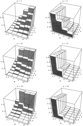
samples were simulated. For each simulated sample, the estima- tors described above were calculated. The results for n

= 200 were very similar to those for n = 100 and are not shown.

The results from our simulations, summarized in Fig- ures 1-5, suggest behavior rather different from that reported by MILLIGAN

.

In fact, the estimators have poor properties for a large range of parameter values. Take the estimators of s, first. It is clear from inspection of

(

17)

that SH yields a negative estimate of the selfing rate if H,“

<

Hb. Likewise, ( 11 ) shows that s:C. gives a negative estimate if S,,

>

S,.

One might think that this should only happen rarely, at least for reasonable sam- ple sizes, but as illustrated by Figure 1, which shows the frequency of simulated samples that give negative estimates of s for various real parameter values, this is not so. It is natural to take a negative estimate of s to be zero (and this was done in our simulations) , even at the cost of introducing bias. Note also the frequency of samples that yield no estimate of s at all because S,

= s b = 0 (Figure 1, right column) . The estimators

of

8

are much better behaved in these respects. The homozygosity estimator

gH

cannot be used when Hb = 0 , but this was observed only very rarely ( <0.3% of the samples) for n = 10 and never for n = 50 or greater.

The bias of the estimators of s is shown in Figure 2.

It is clear that both estimators have similar properties, although the bias of the homozygosity estimator iH is always smaller. In general, the bias is worse the smaller the value of

8.

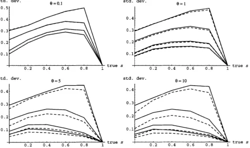
Of course, increasing the sample size always helps, albeit very slowly. The standard deviations of & and SH are compared in Figure 3. Again, both estimators have similar properties in general, although

fH is clearly superior. The bias and standard deviation of the estimators of

8

are shown in Figure 4. The homo- zygosity estimator, O H , is unquestionably inferior, ex- cept perhaps for small values of s and high 8, in which case it is more biased but has smaller variance.

Maximum-likelihood estimates: For moderate to large sample sizes, maximum-likelihood estimates should be superior to those based on moments. The structure of the process described above allows the like- lihood in the model with selfing to be written in terms of likelihoods for models with random mating. Loosely speaking, one simply has to allow for the extra ran- domness involved in initial instantaneous coalescences. Suppose the data, I), consists of sequences from n

diploid individuals. Write m for the number of homozy- gous individuals and /)* for the 2 ( n - m ) alleles sam- pled in the non-homozygous individuals. Among the

m homozygous individuals, write k for the number of different alleles ( k 5 m ) . Label these alleles A , ,

.

.

.

,

Ah and write m 2 , i = 1, 2,

. . .

, k for the number of A , A ,

homozygotes. In other words,

-

I1 = AIAI. * AlAl A2A2. * * A2A2. *

” m l l z n m m2 1 2 W A

’ ’ AkA, I)*. (19)

-

rnk timer

Re-parameterize, and write $ = ( 1 - s / 2 ) 8. Then the likelihood I ( s, @, n ) for s and rC, with data

D

is

where B ( n ,

p ,

x)

is the probability that a Binomial ( n ,

p )

random variable will take the value

x,

7)i,,...,y

is a data set formed from I) by taking I)* and

Z;

+

2 ( ml - i,)

copies of allele AJ, j = 1,

. .

, , k , i.e.,

Aka * Ak * * AkAkY)*, (21 )

“

tk 1imr.s r q - zk tmles

and I, (<,

D )

is the usual coalescent likelihood function with data I ) and mutation parameter 0 =

E .

Computer programs for evaluating this function are available

n = 2

Coalescent With Selfing

n = 2

1189

n = 10 n = 10

n = 5 0 n = 5 0

FIGURE 1.-The fraction of simulated samples that yield negative estimates (left column) or no estimate (right column) using

&.

The homozygosity estimator .iH behaves similarly.

We wrote such a program, using code kindly provided by

R.

C . GRIFFITHS to calculate 1,. Figures 6 and

7

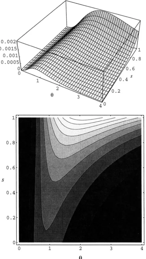
show examples of likelihood surfaces produced using our program. Notice that the surface is much flatter in the s than in the

8

direction, indicating that the estimate of s is considerably more uncertain. Unfortunately, eval- uating expression ( 2 0 ) is extremely timeconsuming because it involves a large number of calculations of

I,,

each of which is quite timeconsuming. For example, for typical samples of size n = 20, evaluation took on the order of days to weeks on a workstation. We are therefore unable to compare the properties of this esti-

1190 M. Nordborg and P. Donnelly

estimated s

estimated s

e=o.1

e =

1

1.

0 . 6 .

true s / . . .

0 . 2 0 . 4 0 . 6 0 . 8 1

' ' _{true s}

estimated s estimated s

e = 5

e =

10

0.8

I/

0.2 0.4 0.6 0 . 8 1 true s true s

FIGURE 2.-Expectation of the moment estimators of s as a function of the actual s for various combinations of 6' and n. The straight line gives the unbiased expectation; the solid lines, results for fs; and the dashed lines, results for 1., For both estimators, results are plotted for n = 2 (largest bias), 10, 50, and 100 (smallest bias).

std. dev.

e

= 0.1 std. dev.

0.

0 .

0 .

0.

0 .

0.2 0.4 0.6 0 . 8 1 true s 0 . 2 0.4 0 . 6 0 . 8 1

std. dev. std. dev.

e = 5

e =

10

0 .

0 .

0 .

0 .

true s

0 - 4 y - 1

0.3

,

,

"""

0.2

I,?

"""

true s

true s

FIGURE 3.-Standard deviations of the moment estimators of s as functions of the actual s values for various combinations of

Coalescent With Selfing 1191

estimated 8

true 8

estimated 8

s = 0.6

est imated 8

s = o

2 4 6 8 10

estimated 8

s = 0.6

estimated 8

s = l

true 8

t

is"^

10 2 4 6 8

. _{true 8}

10 estimated

8

s = 1

true 1

e

true 8

2 4 6 8 10

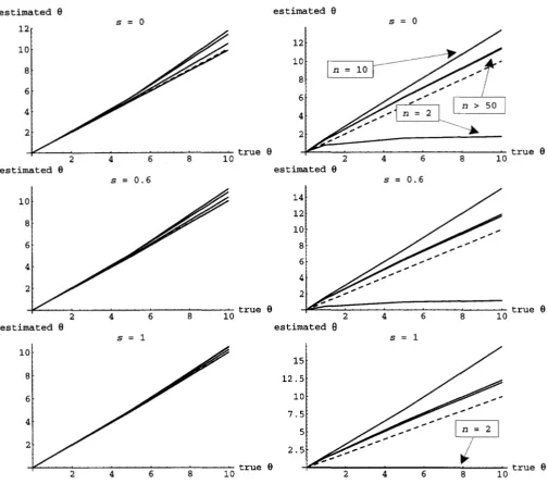
FIGURE 4.-Expectation of the _moment estimators of 8 as-a function of the actual 8 for various combinations of s and n. The left column gives the results for Os and the right those for O H . The dashed line gives the unbiased expectation. Results for s = 0.4 and s = 0.8 are not shown but are very similar. For both estimators, results are plotted for n = 2 (largest bias), 10, 50, and 100 (least bias). Note that when n = 2, 8, exhibits negative bias rather than positive bias (and that it equals zero when n = 2

and s = 1 ) .

( BERGER and WOLPERT 1988)

,

the likelihood surface contains all of the information about the parameters in the data.

DISCUSSION

The coalescent with selfing: We have shown that par- tial selfing can be incorporated into a coalescent frame- work without difficulty, essentially because the ancestral process decomposes into two different processes, a “slow” one that consists of common ancestor events among individuals in a population, and a “fast” one that consists of common ancestor events among alleles within individuals.

Estimation: Using this theory, we have been able to assess correctly the properties of the estimators for sand

0 proposed in MILLIGAN (1996) and above. MILLIGAN estimated variance and bias by repeatedly drawing from the distribution of pairwise coalescent times without regard for the positive correlations induced by the un- derlying genealogy of a real sample. This is inappropri- ate, and we note the almost complete lack of correspon- dence, for example, between his estimates of the vari- ance of fs (Figures

4

and 5, p. 624) and ours (Fig- ure 3 ) .

1192 M. Nordborg and P. Donnelly

std. dev.

10

8

s = o

std. dev.

s = 0.4

std. dev.

12.5 15

I

s = l

10.

2 4 6 8

. _{true 8}

10

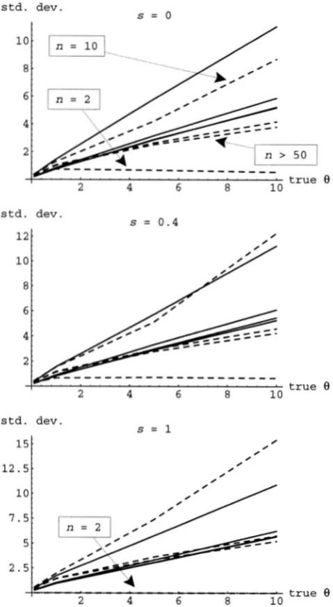
FIGURE 5.-Standard deviation of the moment estimators of

O

as a function of the actual

O

for the same combinations

of sand n used in Figure 4. The solid lines give the results for Os, and the dashed lines give those for Orr.

mate s (BROWN and ALLARD 1970; BROWN 1990)

.

" h e n we estimate sand Bjointly, we are estimating parameters of the two very different processes into which the coales- cent with partial selfing decomposes: the "fast" process, which provides information about s only, and the "slow" one, which provides information about the pa- rameter (cr = ( 2

-

s)

8/2, in which

8 and

s are con- founded. This can be seen from the likelihood function ( 2 0 ) , which loosely consists of a sum of "binomial- like" probabilities multiplied by coalescent likelihoods. Knowing this, the observed behavior of the estimators becomes easy to understand. Since information about

s is available from the fast, binomial-like process, we might expect the variance of the estimate to decrease in the typical ( n" ) fashion of independent observa- tions with increased sample size. This is precisely what

1

0.8

0.6

S

0 . 4

0.;

c

0 1 2 3 4

e

FIGURE 6.-Likelihood surface for s and 0 for a simulated sample of size n = 10. The actual parameter values are s =

0.9, 0 + = 2. For this sample, .fs = 0.96, 8, = 2.72, and & =

0.93, O r / = 7.00.

we see in Figure 3, which gives the standard deviations of the moment estimators of s. The situation is rather different for estimation of 8. Even in the random-mat- ing case, it is well known that increasing the sample size does not, in general, provide much extra information for estimating the scaled mutation rate, here (cr (DON-

NELLY and T A V A K ~ 1995). Indeed, estimators based on pairwise measures, such as the moment estimators dis- cussed here, are not necessarily even consistent. Estima- tion of 8 is more difficult than estimation of (cr because of the confounding with s and the initial randomness induced by the fast process. Figure 5 shows that, as expected, the standard deviations of the moment esti- mators of

8 do not decrease much with increased

n.

Coalescent With Selfing 1193

1

0.8

0.6

S

0 . 4

0 . 2

0

I

4 ”

1

0 . 8

0.6

S

0.4

0 . 9

c

1.5

1.

5.

3 1 2 3

0

FIGURE 7.-Likelihood surface for s and 0 for a simulated

sample of size n = 10. The actual parameter value? are s = 0.9, 19 = 2, as-in Figure 6. For this sample, f5 = 1 ,

Hs

= 3.73,

and .j,, = 1 , H l r = 1.7.5.

estimates (Figures 6 - 8 ) . For the likelihood surfaces we examined, estimation of 0 with s assumed known is ro- bust to the value of s, and conversely. Furthermore, reporting of the likelihood surface is considerably more informative than simply providing point estimates. For asymmetric surfaces ( P.R., Figure 6 ) , even standard in- terval estimates could be quite misleading.

Robustness: MILLICAN assumes a constant popula-

tion size and notes that his results are insensitive to the exact value of that constant size. It does not follow, as

he claims ( p . 620 and p. 626), that the results are insensitive to the assumption of constant population size. In fact, an extension of the argument given above should show that the standard theory for the coalescent with varying population sizes ( DONNELL-Y and T A V A R ~ 1995) (with modifications analogous to those above) will apply to the coalescent with partial selfing as well.

0

0

FIGURI.: 8.-Likelihood surface for s and

H

for a simulated sample of size n = 20. The actual parameter-values are again

s = 0.9, = 2. For this sample, = 0.98,

H,%

= 7.03, and f,, = 0.92,

H,,

= 4.56.

We have not assessed the estimators in this more gen- eral setting, but dependence on the population size process would certainly be expected.

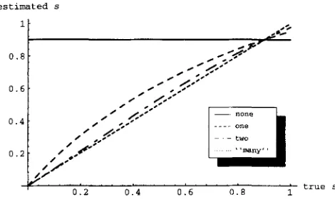
MILLICAN also argues that his method estimates the long-term mating system,” rather than being “based on the segregation of alleles during a single generation of mating.” In fact, the opposite is true. Most of the information about s comes from the association of al- leles within individuals, and this information only re- flects the last few generations. This is easily seen, for instance, by considering how data from the coalescent with partial selfing is simulated (see above). Going backward in time, pairs of alleles sampled within indi- viduals either coalesce instantly, o r become part of a standard, haploid coalescent with an appropriate time- scale. This point is further illustrated by Figure 9, where the expectation of .fv is plotted against the actual value of s under the last few generations. It is clear that the

1194 M. Nordborg and P. Donnelly

estimated s

I t

,

/

I

/ 0 -

I

0.2 0 . 4 0 . 6 0.8

i

true

FIGURE 9.-Sensitivity of the estimated selfing rate to

changes in s. The “long-term” value of s is 0.9, and curves show the expectation of j’s given that the actual value of s was

that on the abscissa in the preceding few generations, where “few” is 0, 1, 2, or “many” ( i.e., when the long-term value is

the one on the abscissa).

estimated s almost exclusively reflects the value of s in the preceding generation, and that the “long-term” mating system is largely irrelevant to the estimate. Note that the same argument applies to the other estimators discussed above.

It can be shown that in a model in which the selfing rate vanes independently from generation to genera- tion the behavior of the slow process in the coalescent with selfing is as described above, with s replaced by the mean of the distribution of selfing rates. The behav- ior of the fast process, and hence of the estimators, on the other hand, is quite sensitive to varying selfing rates. While the actual value of an estimator for s will be heavily dependent on the actual values of the selfing rate over the last few years, the sampling properties will depend sensitively on the entire distribution of possible values for the selfing rate over the same period.

All results derived here assume a single neutral locus. It is worth pointing out that selection on linked loci may have a very strong effect on the variability at neutral loci, either in reducing it through processes such as background selection ( CHARLESWORTH et al. 1993) and selective sweeps (MAYNARD SMITH and HAICH 1974;

KAPLAN et al. 1989), or in increasing it through some form of balancing selection ( STROBECK 1983; HUDSON and &WLAN 1988; KAPLAN et al. 1988; NORDBORG et al. 1996), and that all these effects will be stronger under selfing ( NORDBORC et al. 1 9 9 6 ) .

Conclusion: Coalescent-based estimates do not pro- vide a magic bullet when it comes to estimating the selfing rate. As we have seen, the problem of recent fluctuations in the degree of selfing is in no sense avoided. Furthermore, collecting data to estimate both s and

0

involves a contradiction: to estimate s, we want simple data ( the genotype) from large number of indi- viduals, whereas to estimate 8 we need detailed data ( a sequence or several sequences) fromjust a few individu- als ( PLUZHNIKOV and DONNELLY 1 9 9 6 ) . Because DNA

sequence data provide more certain information about the genotype than do data based on classical markers

such as allozymes, it is certainly preferable, ceterisparibus

(in particular, the sample size needs to be roughly simi- lar) , but if moment estimators of s are of primary inter- est, not much is gained.

We thank BRIAN CHARLESWORTH, DEBORAH CHARLESWORTH, I”

TIN MBHLE, and especially TOM NAGWAIU for helpful discussions and comments on the manuscript. M.N. was supported by U.S. Na- tional Science Foundation grant DEB 92-17683 to DEBORAH CHARLESWORTH. P.D. was supported in part by U.S. National Science Foundation grant DMS 95-05129, the Block Fund of the university of Chicago, and U.K. Engineering and Physical Sciences Research Council Advanced Fellowship B/AF/ 1255.

LITERATURE CITED

BERGER, J. O., and R. L. WOLPERT, 1988 TheLikelihoodPrinciple. Insti- tute of Mathematical Statistics, Hayward, C A .

BROWN, A. H. D., 1990 Genetic characterization of plant mating sys- tems, pp. 145-162 in Plant Population Genetics, Breeding, and Ge- netic Resources, edited by A. H. D. BROWN, M. T. CLEGG, A. L.

KAHLER and B. S. WEIR. Sinauer Associates, Sunderland, MA. BROWN, A. H. D., and R. W. A L ~1970 Estimation of the mating ,

system in open-pollinated maize populations using isozyme poly- morphisms. Genetics 66: 133-145.

CHARLESWORTH, B., M.T. MORGAN and D. CHARLESWORTH, 1993 The effect of deleterious mutations on neutral molecular varia- tion. Genetics 134 1289-1303.

DONNELLY, P., and S. TAV&, 1995 Coalescents and genealogical structure under neutrality. Annu. Rev. Genet. 2 9 401-421. GRIFFITHS, R. C., and S. TAVXR~, 1994a Ancestral inference in popu-

lation genetics. Stat. Sci. 9 307-319.

GRIFFITHS, R. C., and S. TAV&, 1994b Sampling theory for neutral alleles in a varying environment. Philos. Trans. R. SOC. Lond. B 344: 403-10.

GRIFFITHS, R. C., and S. TAV&, 1994c Simulating probability distri- butions in the coalescent. Theor. Popul. Biol. 46: 131-159. HALDANE, J. B. S., 1924 A mathematical theory of natural and artifi-

cial selection. Part 11. Proc. Camb. Phil. SOC., Biol. Sci. 1: 158- 163.

HUDSON, R. R., 1990 Gene genealogies and the coalescent process, pp. 1-43 in Oxford Surveys in Evolutionaly Biology, edited by D.

FUTUYMA and J. ANTONOVICS. Oxford University Press, Oxford. HUDSON, R. R., and N. L. K A P I ~ , 1988 The coalescent process in models with selection and recombination. Genetics 120: 831- 840.

KAPIAN, N. L., T. DAARDEN and R. R. HUDSON, 1988 The coalescent process in models with selection. Genetics 120: 819-829. KAPIAN, N. L., R. R. HUDSON and C. H. LANGLEY, 1989 The “hitch-

hiking” effect revisited. Genetics 123: 887-899.

KINGMAN, J. F. C., 1982a The coalescent. Stochast. Proc. Appl. 13:

KINGMAN, J. F. C., 1982b Exchangeability and the evolution of large populations, pp. 97-1 12 in Exchangeability in Probability and Statis-

tics, edited by G. KOCH and F. SPI~ZICHINO. North-Holland P u b lishing Company, Amsterdam.

KINGMAN, J . F. C., 1982c On the genealogy of large populations. j.

Appl. Prob. 19A 27-43.

KUHNER, M. R, J. YAMATO and J. FEISENSTEIN, 1995 Estimating ef-

fective population size and mutation rate from sequence data using Metropolis-Hastings sampling. Genetics 140: 1421 -1430. LI, C. C., 1955 Population Genetics. University of Chicago Press, Chi-

MAYNARD SMITH, J., and J. HAIGH, 1974 The hitchhiking effect of a favourable gene. Genet. Res. 23: 23-35.

M I L L I G ~ , B. G., 1996 Estimating long-term mating systems using DNA sequences. Genetics 142: 619-627.

MOHLE, M., 1996 Coalescent results for diploid population models and the coalescent with selfing. Technical Report 433, Depart- ment of Statistics, The University of Chicago, Chicago. NORDBORC, M., B. CHARIESWORTH and D. CHARLESWORTH, 1996 In-

creased levels of polymorphism surrounding selectively main- tained sites in highly selfing species. Proc. R. SOC. Lond. B 263: 1033-1039.

235-248.

Coalescent With Selfing 1195

PLUZHNIKOV, A,, and P. DONNELLY, 1996 Optimal sequencing strate- locus linked to a chromosomal arrangement. Genetics 103: 545-

gies for surveying molecular genetic diversity. Genetics 144: 555.

1247-1262. TAV&, S., 1984 Line-ofdescent and genealogical processes, and

POW E., 1987 On the theoly of partially inbreeding finite popula- their applications in population genetic models. Theor. Popul.

STEWART, F. M., 1976 Variability in the amount of heterozygosity WRIGHT, S., 1969 Evolution and the Genetics ofpopuhtions, vol. 2.

tions. I. Partial selfing. Genetics 117: 353-360. Biol. 2 6 119-164.

maintained by neutral mutations. Theor. Popul. Biol. 9: 188- University of Chicago Press, Chicago.

201.