A Tabu Search Algorithm for the Steiner Tree Problem.

ABSTRACT

KULKARNI, GIRISH. A Tabu Search Algorithm for the Steiner Tree Problem. (Under

the direction of Professor Yahya Fathi.)

The Steiner Tree problem in graphs is an NP-hard problem having applications in many

areas including telecommunication, distribution and transportation systems. We survey,

briefly, a few exact methods and a few heuristic approaches that have been proposed for

solving this problem. Further, we propose a tabu search algorithm whose key feature

includes a neighborhood definition consisting of exchange of key paths. The algorithm is

empirically tested by running computational experiments on problem sets, with known

optimal values, that are available over the internet. The results from the tabu search are

compared with the optimal values and with the results of a well-known heuristic

procedure. The experimental results show that the tabu search algorithm is reasonably

successful. It produces near-optimal solutions in the experiments conducted and performs

better than the heuristic procedure. We also explore other avenues for future work and

BIOGRAPHY

Girish Kulkarni was born on the 1st of November 1976 in the beautiful coastal city of Margao in the state of Goa, India. After completing his schooling in Mumbai, he obtained the Bachelor of Technology degree in Metallurgical Engineering and Materials Science from IIT Bombay. Before joining the Operations Research program at NCSU , he worked as a software engineer for a year at Infosys Technologies Ltd in Pune, India.

ACKNOWLEDGEMENTS

First and foremost, I would like to thank my parents Dr. Suneela Kulkarni and Dr.

Mangesh Kulkarni whose support and encouragement has led me to success. I would also

like to thank my advisor Dr. Yahya Fathi for his advice and painstaking guidance. I am

grateful to my committee members Dr Stephen Roberts and Dr. George Rouskas for their

encouragement and feedback.

I would also like to mention my friends Prashant, Rajesh, Bobby and Sai and finally, last

but not the least, I would like to thank my room mates, Prabhas Sinha and Vijay Iyer, for

TABLE OF CONTENTS

LIST OF FIGURES ... vi

LIST OF TABLES... vii

1 INTRODUCTION ... 1

1.1THE STEINER TREE PROBLEM... 1

1.2 PROBLEM DEFINITION... 2

1.3COMPLEXITY... 3

1.4 APPLICATIONS... 4

2 LITERATURE SURVEY... 5

2.1 EXACT METHODS... 5

2.1.1 Spanning Tree enumeration... 5

2.1.2 Branch and Bound method for the steiner tree problem... 6

2.2 HEURISTIC TECHNIQUES... 9

2.2.1 The Cheapest Insertion Heuristic ... 9

2.2.2 The Pilot Method ... 12

2.2.3 Local Search Methods ... 13

2.2.4 Simulated Annealing and Genetic Algorithms... 14

2.2.5 Tabu Search... 15

2.2.6 A New Tabu Search Algorithm ... 16

3 TABU SEARCH... 18

3.2 DATA STRUCTURES... 19

3.3 NEIGHBORHOOD STRUCTURE... 20

3.4 SEARCH STRATEGY... 21

3.5 EVALUATION OF OBJECTIVE... 21

3.6 TABU LIST AND ASPIRATION CRITERIA... 22

3.7 DIVERSIFICATION STRATEGY... 23

3.8 STARTING SOLUTION AND STOPPING CRITERION... 24

3.9 PARAMETER SELECTION... 25

3.9.1 Tabu Tenure ... 25

3.9.2 Number of iterations before diversification... 28

3.10 PSEUDO-CODE FOR THE TABU SEARCH... 30

4 COMPUTATIONAL EXPERIMENTS ... 33

4.1 PROBLEM SETS... 33

4.2PERFORMANCE MEASURES... 34

4.3 OBSERVATIONS... 35

4.3.1 Comparison with optimal values ... 36

4.3.2 Comparison of CHINS-V with TS ... 40

4.4CONCLUDING REMARKS... 44

5 SUMMARY AND AVENUES FOR FUTURE WORK ... 45

REFERENCES ... 48

APPENDIX 1A... 50

List of Figures

FIG 1 THE CHEAPEST INSERTION HEURISTIC (CHINS)... 11

FIG 2RELATING SOLUTION QUALITY WITH THE TABU TENURE... 28

FIG 3 RELATING MAXITERTILLDIVERSIFY WITH SOLUTION QUALITY... 29

List of Tables

TABLE 1 SUMMARY OF RESULTS FOR PROBLEM SET I080... 38

TABLE 2 SUMMARY OF RESULTS FOR PROBLEM SET I160... 39

TABLE 3A COMPARISON OF CHINS-V WITH TS FOR SET I080 ... 42

TABLE 3B COMPARISON OF CHINS-V WITH TS FOR SET I080 ... 42

TABLE 4A COMPARISON BETWEEN CHINS-V AND TS FOR SET I160... 43

1 Introduction

1.1 The Steiner Tree Problem

The Steiner Tree Problem involves constructing the least cost network that spans a given

set of points. The novelty of the Steiner Tree Problem is that new auxiliary points can be

introduced between the original points so that the spanning tree of all the points will be of

lower cost than otherwise possible. The Steiner Tree Problem can be categorized into

three major areas: the Euclidean Steiner Tree Problem (SPE), the Rectilinear Steiner

Tree Problem (SPR) and the Steiner Tree Problem in Graphs (SPG). Here, we focus our

attention only on the SPG, which is a combinatorial version of the Steiner Tree Problem.

Henceforth, in this text we will refer to the SPG as the steiner tree problem.

A large amount of literature concerning the various aspects of the steiner tree problem

exists and it includes exact methods as well as various heuristic techniques. Here, we

propose a new tabu search algorithm for solving the steiner tree problem. In this chapter,

we give the exact problem definition along with an introduction to the terminology and

notation used in the remainder of the text. The applications and the computational

literature with emphasis on the ideas that are relevant to the tabu search algorithm that

has been developed here. First, the Cheapest Insertion heuristic is explained along with a

few of its multiple pass variants. Then we briefly discuss a meta-heuristic strategy called

the pilot method. We also touch upon other meta-heuristic approaches like simulated

annealing and genetic algorithms and lastly the motivation behind the tabu search

algorithm that we propose is given. Chapter 3 describes the various aspects of the tabu

search algorithm, including the pseudo-code and experiments that led to selection of the

various parameter values. Chapter 4 presents the results of the experiments conducted to

test the tabu search algorithm. The tabu search results are compared to known optimal

solutions of two sets of problem instances. Furthermore the tabu search is compared with

another heuristic method. Chapter 5 mainly talks about avenues and ideas for future

work.

1.2 Problem Definition

The steiner tree problem can be defined as follows.

Given: An undirected graph G = (V, E, w), where, w: E →R is a non-negative weight

function and a non-empty set N of terminals, N⊆V. Here V denotes the set of all nodes present in the graph and E represents the set of all edges present in the graph. The graph

G consists of two sets of nodes, the set of terminals denoted by N, and a set of

non-terminals denoted by Q, i.e., Q = {v: v ∈V/N}. Find: sub-graph Tg of G such that:

1) Each pair of terminals is linked through a path in Tg.

The sub-graph Tg consists of all terminal nodes N of G and some non-terminal nodes.

These non-terminal nodes which are present in the sub-graph Tg are called steiner nodes

or steiner vertices. The sub-graph Tg obtained is known as the steiner minimal network (it

should be referred to as the steiner minimum network, however for historical reasons the

less correct term is used). If all the edge weights are positive, the steiner minimum

network has to be a tree and hence the problem is often referred to in the literature as the

steiner tree problem and Tg is often called the steiner minimal tree. Throughout our

discussion we will refer to the optimal solution as the steiner minimum tree and a

sub-optimal solution as the steiner tree. |N| represents the number of terminals, |V| the number

of vertices and |E| the number of edges. The graph will be represented as G and any tree

will be represented as T. VT, ET and NT represent the set of all nodes, all edges and all

terminals in the tree T, respectively. If T represents a legitimate solution then N = NT. A

path in any graph G having end nodes ui and vi and intermediate nodes x1, x2, x3, …, xk

is denoted by P(ui,…,vi). The total length of this path is represented by c(P) or by d(vi,ui).

Similarly the total length of any tree T is represented by c(T).

1.3 Complexity

Some well known special cases of the steiner tree problem can be solved in polynomial

time. When |N| = 2 the problem reduces to the shortest path problem while when N = V

the problem reduces to the minimum spanning tree problem. Both these problems can be

solved in polynomial time. On the other hand, a large number of special cases have been

graph, a bipartite graph or a complete graph with edge weights either 1 or 2. Thus in the

general case the problem is an NP-hard problem. However the complexity of the problem

in some special cases like that of planar graphs with all edges of weight 1 has not yet

been settled. [6]

1.4 Applications

The steiner tree problem has numerous applications especially in the areas of

telecommunication, distribution and transportation systems. The computation of

phylogenetic trees in biology and the routing phase in VLSI design are real life problems

that have been modeled as the steiner tree problem [6]. Minimization of the cost of trees

generated as a solution for multicast routing in communication networks have been

traditionally formulated as the steiner tree problem. Another interesting application is

based on the billing strategies of large telecommunications network service providers.

The bill isn’t based on the actual number of circuits provided, which may change over a

period of time, but on the basis of a simple formula calculated for an ideal network which

will provide all the facilities at minimum cost. Moreover, several network design

2 Literature Survey

2.1 Exact Methods

Many exact methods for optimal solutions for the steiner tree problem have been

proposed in the literature. Hwang et al. [6] give a comprehensive overview of the many

approaches including enumeration schemes, branch and bound methods, dynamic

programming as well as mathematical programming formulations. Here, two methods,

the spanning tree enumeration and a branch and bound algorithm are explained.

2.1.1 Spanning Tree enumeration

This algorithm was proposed by Hakimi [5] and a modification was proposed by Lawler

[8] based on the observation that finding a steiner minimum tree for N in graph G is

equivalent to finding a steiner minimum tree for N in the distance network induced by all

vertices V in graph G. This enumeration is based on two results [6]

1) There exists a steiner minimum tree for |N| terminals in a given distance network

where each steiner vertex has degree of at least 3.

2) There exists a steiner minimum tree for |N| terminals in a given distance network with

This enumeration procedure involves enumerating minimum spanning trees of

sub-networks induced by supersets of the |N| terminals of size at most 2|N| – 2.

The number of minimum spanning trees that must be determined is given by

Here, denotes “n choose k” and so = n!/(n-k)! k!.

The execution time of this algorithm is asymptotically upper bounded by (|N|2 . 2(|V|-|N|) ₊

|V|3) i.e. time complexity is given by O(by (|N|2 . 2(|V|-|N|) _{+ |V|}3_{) [6]. The term |V|}3 _comes

form the Floyd-Warshall algorithm used to compute the shortest path from each vertex to

all other vertices.

2.1.2 Branch and Bound method for the steiner tree problem

Many branch and bound algorithms are available in literature to optimally solve the

steiner tree problem. Here we briefly describe the algorithm proposed by Shore et al. [11]

For a graph G, let F0 represent the set of all feasible solutions (all trees spanning the set

of terminals N). The branch and bound algorithm proceeds by systematically partitioning

the set F0 into subsets. These subsets are investigated using upper and lower bounds to

k

n

k

n

≤

2

i=0

|N|-2

check whether they can contain a steiner minimum tree. Let Fi be one such subset. Fi is

characterized by two sets of edges INi and OUTi. The set INi contains all the edges that

have to be present in all solutions belonging to Fi. OUTi,on the other hand, contains all

those edges that are not permitted in any solution present in set Fi. Initially, for F0, IN0 =

Φ (empty set) and OUT0 = Φ.

For any subset Fi, the graph Gi is obtained by removing from G all edges belonging to

OUTi and contracting the edges belonging to INi. Contraction of an edge is a process in

which the edge and its end nodes are replaced by a single node and this node is marked as

being a terminal node. Contracting an edge ei is one way of ensuring that every solution

Ti contains edge ei. Thus, by reducing graph G to Gi, each edge of INi is forcibly included

in every solution Ti and every edge in OUTi is excluded from Ti. Let Ni be the set of

terminals in Gi. Finding the steiner minimum tree for the graph G is equivalent to finding

the steiner minimum tree Ti, for all terminals of Ni in graph Gi. First, an upper bound Bi

for set Fi can be determined by adding the lengths of edges in INi to the length of a tree

spanning Ni in Gi obtained by any of the steiner tree heuristics described in section 2.2.

Let cmin be the length of the shortest tree spanning all the terminals found till date. At the

start of the branch and bound algorithm, cmin = ∞, and at any later stage if cmin > Bi then

cmin is set equal to the upper bound Bi.

In order to find a lower bound bi for Fi, we define the following

• wni is the length of the shortest edge incident on ni, where ni ∈Ni

• w'

ni is the length of the shortest edge between ni and nk, where ni and nk∈Ni

and c(Ti) is the total length of all edges in Ti. Thus given a terminal ni we have a notation

for the shortest and second shortest edge incident on it and the shortest edge between ni

and any other terminal.

We consider two cases while trying to find a lower bound. The first case is when Ti

contains at least one steiner node then it has atleast |Ni| edges and each terminal ni ∈Ni is

incident on atleast one edge in Ti. We can now define a quantity

t

Thus ti is the sum of the weights of the shortest edge incident on each terminal ni. The

second case is when Ti contains only terminals, then Ti has |Ni| -1 edges. For this case we

define the quantity

t

Now, the quantities

t

t

If cmin ≤ bi, then no tree in Fi can be shorter than the shortest tree found so far and so

there is no need to partition the set Fi any further. A solution is a feasible solution when

all the terminals present in Ni are connected to each other in the solution Ti only with

edges from INi. Whenever it is uncertain whether Fi contains a steinerminimum tree, it is

partitioned into two subsets for a suitably chosen edge em∈E\ (INi∪OUTi ):

Fj : where INj = INi∪ em, OUTj = OUTi

t

=

Σ

w

≤

c(T

)

t

=

Σ

w

- min (w

| n

∈

N

)

≤

c(T

)

nj∈Ni

b

= min(t

, t

) +

c (e

)

Fk: where INk = INi, OUTk = OUTi∪ em

The choice of em is crucial to the performance of the algorithm. The authors select as em,

the minimum length edge incident with a terminal nj ∈ Ni for which (w~nj - wnj) is

maximum. Fj is examined first and a steiner tree is found for Fj or it is established that an

optimal feasible solution cannot be found in Fj. Then Fk is examined and the algorithm

backtracks to Fi. The minimum length steiner tree found while the algorithm backtracks

to F0 is the solution.

2.2 Heuristic Techniques

Various approaches have been used to develop heuristics for the steiner tree problem. A

comprehensive review of these heuristics is presented by Hwang et al. [6] and more

recently by Voss [14]. Most of these heuristic methods are constructive methods and can

be classified on the basis of a common characteristic in their approach. Some heuristics

follow the path-based approach, there are others that are vertex-based and still others that

can be considered to be tree based heuristics. Furthermore, there exist a number of other

heuristics that do not fall in any of the above categories such as the contraction heuristic

or the dual ascent heuristic. These constructive heuristics give rise to important ideas and

many of the ideas for neighborhood definitions and solution representations have their

origins in these constructive heuristics. Theoretically, nearly all heuristics have a worst

case upper bound of 2. One variation of the shortest distance graph heuristic has been

2.2.1 The Cheapest Insertion Heuristic

Below, we briefly describe a constructive heuristic originally proposed by Takahashi and

Matsuyama [13]. This heuristic, which will be referred to as CHINS henceforth, is based

on Prims’s algorithm for finding the minimum spanning tree in a graph. The authors have

also shown that the length of the steiner tree obtained using the CHINS heuristic

c(TCHINS) is bounded. The bound is also proved to be tight and is given by

c(TCHINS)/c(Topt) ≤ 2 – 2/|N| for any graph G and any set of terminals N.

The shortest Path heuristic involves the following steps

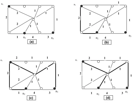
1. Begin by choosing an arbitrary terminal nk and include it in the tree T. T is the current

partial solution and contains only one vertex: the terminal nk. Let k= 1. (Fig 1 a)

2. If k = |N| then Stop. Else determine a terminal nk+1 that is closest to the current

solution T. Add to T all the vertices on the shortest path from nk+1 to T. (Fig 1 b)

k = k+ 1. Repeat.

3. Find a minimum spanning tree for the sub-graph induced by the nodes in T. (Fig 1

d)

4. Remove from the minimum spanning tree non-terminals of degree 1, one at a time.

Fig 1 The cheapest insertion heuristic (CHINS)

This heuristic is sensitive to the choice of initial solution and so it needs to be repetitively

applied. Some strategies that have been suggested for repetitive runs of this heuristic are

CHINS – N : Begin each run with a different terminal. Total number of runs = |N|

CHINS – V : Begin each run with a different vertex. Total number of runs = |V|

CHINS – nV : Fix a terminal ni . Begin each run with the shortest path from a terminal

nk (k ≠i) to ni. Total number of runs = N –1.

CHINS – NN :Begin each run with the shortest path from a different pair of terminals.

Total number of runs = N (N – 1).

2 1 1

2

1

1

1 2

4 3

1

(a)

n1

n2 n₃

2

2

1 1

1 1 2 1 1 1 2

4 3

1

(c)

n1

n2 n3

2

2

1 1

1 1 2 1 1 1 2

4 3

2.2.2 The Pilot Method

The pilot strategy proposed by Cees Duin and Stefan Voss [2] is a meta heuristic

approach which can be applied for solving the steiner tree problem. This meta-heuristic

has been proposed by the authors to enable, without much effort, a tradeoff between

computation time and accuracy. For NP-hard problems heuristics exist that solve the

problem in polynomial time using quick greedy rules to incrementally construct a

solution. These greedy rules are often myopic and do not take into account the long term

effect of a decision and hence such constructive heuristics often return reasonable but not

near-optimal solutions. It would be extremely beneficial if it were possible to take into

account how present decisions affect later choices in the algorithm. The pilot heuristic

strategy is one such look-ahead method. A similar strategy has been used in the area of

artificial intelligence where there is an evaluation of a decision with respect to the

likelihood of that decision yielding a good solution in the future and to prune away those

decisions which are not likely to be promising. The authors call this approach a tempered

greedy approach and it is meta-heuristic in the sense that it can be formulated to suit all

kinds of combinatorial problems.

In the pilot strategy, a combinatorial optimization problem is tackled by using multiple

passes of an existing heuristic that is called the pilot heuristic. The pilot heuristic is used

to build step-by-step a partial solution that is called the “master solution”. Consider that a

partial solution M exists and let there be a number of choices represented by C that can

to extend the partial solution M by changing it in minimal fashion. On the basis of the

changed master solution new pilot calculations are started for each ci ∉ M providing a

new solution element c′0 and so on. The pilot heuristic actually provides an upper bound

on the objective value of the final solution that can be obtained if the choice c0 is chosen.

Suppose the pilot heuristic or the sub-heuristic takes execution time O(nk) then the pilot

method takes time O(nk+2) where n represents problem size and k is a positive integer.

Specifically for the steiner tree problem, a slight modification of the CHINS heuristic

described in section 3.2.1 can be used to formulate a pilot method. At any given time a

partial solution M is a forest covering the vertices of set N. Each tree in this forest can be

considered a component and can be replaced by a single terminal. Initially, M consists of

all the terminals, i.e., it has a total of |N| components. The pilot method proceeds by

running the CHINS heuristic from each vertex v as the starting point. Let v0 be the

starting vertex from which the best objective value is obtained. We now run one step of

the CHINS heuristic from v0. If v0 is a terminal then we look for a component that is

closest to it and create a new one by combining it with vertex v0. If v0 is not a terminal

then we combine v0 with the closest terminal and then repeat this procedure once more to

obtain the new component. This process continues till the partial solution M consists of

only one component that contains all vertices of N.

2.2.3 Local Search Methods

Apart from these constructive heuristics, other techniques such as neural networks, local

algorithms and Tabu Search have also been investigated. Local improvement strategies

are based on two types of transformations: edge oriented transformation and node

oriented transformation. Edge oriented transformations may involve deletion of an edge

from a steiner tree along with the resulting steiner nodes of degree one. The disconnected

components are then connected to each other through the shortest path. In node oriented

transformation all nodes in the graph are classified as in or not in. Critical vertices

(steiner nodes with degree greater than or equal to 3) in the solution are eliminated and

the components are reconnected using the shortest paths. Local improvement approaches

based on the node-oriented strategies are time consuming. This could be because the

search may involve large number of exchanges of steiner nodes of degree 2 without any

change in the objective value. Another reason is the recalculation of minimum spanning

trees at each iteration.

2.2.4 Simulated Annealing and Genetic Algorithms

Quite a few Simulated Annealing [1] and Genetic Algorithm [3] approaches have been

investigated and according to Voss [14] the results indicate that the SA approach can be

effective with respect to solution quality. The most effective SA approach for the steiner

tree problem, implemented by Wade and Rayword-Smith [15], regularly changes its

search space topology by changing the problem representation and related neighborhood

transformation. The solution in a GA can be represented using a bit string of size equal to

the number of non-terminal nodes in the graph. Numerical results show that using

appropriate values of parameters, the optimal solution to small-sized problems can be

of chunking. The general idea of chunking approach is to speed up the process of

evolution by combining chunks of attributes that seem to be superior and to define

schemata being responsible for the solution quality.

2.2.5 Tabu Search

Tabu search heuristics based on the node-oriented neighborhood have been investigated

in a number of papers. Sondergeld and Voss [12] investigate a specific intensification-

diversification approach where the diversification is achieved by scattering multiple

search trajectories over the solution space and intensification is based on strategic restarts

of search strategies on “good” solutions that have been previously encountered. Gendreau

et al. [4] present a Tabu search strategy where the initial solution is constructed using the

cheapest insertion heuristic and the search strategy is based on insertion and deletion of

steiner nodes. The algorithm has a diversification procedure which includes ideas such as,

include steiner nodes previously not part of the solutions, drop the path between nodes

where shortest in-tree distance between the nodes is much larger than the shortest

distance between them in the graph, etc. Another important contribution is the

consideration of efficient data structures for manipulating trees when adding and deleting

nodes, as the computational effort for exploring a neighborhood can be enormous.

Rebeiro et al. [10] have proposed a tabu search algorithm which has similar

neighborhood structure and search strategy as the one mentioned above. In this paper the

authors define procedures by which the neighborhood search is made faster and more

efficient so that comparable solution quality is obtained in considerably smaller execution

2.2.6 A New Tabu Search Algorithm

Voss [14] summarizes the comparison of the various algorithms whose performance on

the problem sets B, C, D and E created by Beasley is available in the literature. For the

local improvement the crucial edge exchange strategy produced better results than the

key path exchange idea when considering quality of solutions. The tabu search strategies

showed markedly better results then the local improvement methods but the results for

different diversification schemes for the tabu search were very close to each other. The

genetic algorithms preformed slightly worse then the tabu search methods. When

reduction techniques were used before the application of GA or tabu search, the results

were much better for both tabu search and GA. Thus published results point out the fact

that the tabu search algorithms show a lot of promise for the steiner tree problem.

Moreover, the edge oriented neighborhood definition for Tabu search still lacks thorough

consideration [14].

We propose a tabu search algorithm based on an edge oriented neighborhood definition

for the undirected steiner tree problem in graphs. This algorithm begins with an initial

solution obtained by running the CHINS heuristic from a starting vertex. The tabu search

improves the solution over a series of iterations. Each iteration investigates all neighbors

of the current solution obtained by a key path exchange mechanism. This mechanism is

performed so that the computation required for the evaluation of each neighbor is

by moving from the current solution to its best neighbor. This procedure is repeated and

terminates when a stopping criterion is met. This algorithm also employs a diversification

procedure that forces the search into unexplored regions of the search space.

The various aspects of this tabu search algorithm are explained in detail in the next

3 Tabu Search

This chapter describes the various aspects of the tabu search algorithm in detail. We

begin with the solution representation and go on to describe the neighborhood structure,

search strategy, tabu list, aspiration criterion, stopping criteria and objective evaluation.

The chapter also includes a description of the diversification procedure and the

pseudo-code for the tabu search.

3.1 Solution Representation

In the context of the tabu search, any tree T that contains all terminal nodes is a solution.

Apart from all the terminal nodes a solution will also contain non-terminal nodes called

steiner nodes. The set of steiner nodes in a solution T, will be referred to as QT, i.e., QT =

{v: v∈Q and v is in T}.

The solution tree T is stored in two formats, the first one is a one dimensional array called

the parent array and the second is a list of arrays called the adjacency list structure. The

solution T can be considered to be a rooted tree and hence each node in T, except the root

node, has another node in T as its parent (or predecessor). The parent array format stores

the complete list of predecessor nodes. The adjacency list is motivated as follows; if a

node u in T is connected to another node v, which also is in T, through a single edge, than

v is a neighbor of u. Thus, every node u in T has an adjacency list that contains all its

adjacency lists of all nodes in T. The parent array structure is important because it helps

in the traversing of all the nodes of the steiner tree. The adjacency list is required because

it is used in the various graph algorithms used as part of the tabu search.

3.2 Data Structures

Firstly, we assume that the nodes are numbered from 1 to |V| in some arbitrary manner.

Let the current solution T, have VT as the set of all nodes, ET as set of all edges and node

sT as the source. We denote the parent array for T by π, where the kth element of π, π(k)

contains the parent (or predecessor) of node k for all k ∈ T and k ≠ sT. For the source

node sT, π(sT) is defined to be equal to sT, i.e., the source node is its own parent. Since the

total number of edges in a tree is one less than the total number of nodes, a parent array

of size |VT| is adequate to store the tree. In this Tabu search implementation, the parent

array has size equal to |V|, the total number of nodes in the graph. For those nodes v of

the graph G which are not in the present solution, i.e., ∀v∈V but v∉VT, we define π(v)

= 0.

The adjacency list Adj, for the steiner tree T, is implemented as an array of |V| arrays, one

for every node in the graph G. For each node u, such that u ∈ VT, the adjacency list

Adj(u) contains all the vertices v such that there is an edge euv joining u to v and euv∈ET.

Thus Adj(u) contains all nodes adjacent to u in the tree T. The vertices in the adjacency

list are stored in arbitrary order. Those nodes k that do not belong to the tree have empty

u equals the number of edges incident on u. Thus, the total space used to store the

adjacency list structure is at least 2(|N| -1).

The graph G itself is stored in two formats one form is the adjacency list described above

and the other data structure is known as the adjacency matrix. The adjacency matrix A of

the graph G is a square matrix with number of rows and columns equal to |V|. If the

weight w of the edge connecting node u to node v is represented by w(u,v), then auv =

w(u,v), when the edge euv∈E, and aij = 0, otherwise.

3.3 Neighborhood Structure

Any intermediate solution occurring during the course of the search is a tree that consists

of all terminal nodes in the graph and some steiner nodes. Based on the degree of the

nodes in the solution T, we classify the nodes in the graph into two types: critical nodes

and non-critical nodes. All steiner nodes of degree greater than 2 and all terminal nodes

are classified as critical nodes. Thus, all non-critical nodes are steiner nodes with degree

exactly equal to 2. Further, we define a key path to be a path in the steiner tree that has

critical nodes as its end points and each intermediate node is a non-critical node. A

steiner tree can be considered to be a minimum spanning tree with critical nodes as

vertices and key paths as edges. When all the steiner nodes are critical nodes, then the

total number of key paths equal the total number of edges in the tree. Hence the

A tree T' is defined as a neighbor of tree T, if T' is constructed from T by removing a

key path from T and reconnecting the two fragments formed with the shortest path

between the two fragments. Every key path Pi in tree T gives rise to a neighbor T' and

hence the total number of neighbors for given steiner tree T equals the total number of

key paths in T. Thus the neighborhood size is at the most |VT|.

3.4 Search Strategy

A single iteration of the tabu search consists of investigating the entire neighborhood of

the current solution and selecting the best non-tabu neighbor. This neighbor is accepted

and used as the current solution for the next iteration. If the best solution in a given

iteration is not an improving solution it is still selected and the search proceeds by

exploring all its neighbors. The algorithm always keeps track of the best ever solution

found in the course of the search.

3.5 Evaluation of Objective

The objective value of a steiner tree is the total weight of all edges in it. To find the

objective value of any given solution T, we need to add up the weights of all the edges in

T. The search strategy involves choosing the neighbor with the best objective value and

this objective value is speedily calculated as follows. At the start of the tabu search the

CHINS heuristic calculates an initial solution Ti and also gives the total edge weight of

Ti. We move from Ti to its neighbor Ti'by dropping an existing key path from the tree Ti

and re-connecting the fragments with another path to obtain Ti'. Now, using the weights

easily find the objective value of T'. Let us denote the difference between the weights of

the dropped path and the added path as δ. Thus δ subtracted from the objective value of Ti will give us the objective value for Ti'. In the neighborhood search, we do not need to

calculate the objective value of each neighbor obtained during the search. The neighbor

T' which corresponds to the highest value of δ is the best neighbor of T.

3.6 Tabu list and Aspiration criteria

The search algorithm searches for the best possible neighbor Tnbr of the current accepted

solution T. The Tabu search will go on to Tnbr even though Tnbr may have objective value

greater than T. This can cause the tabu search to cycle between Tnbr and T unless we

introduce appropriate measures to prevent cycling. To this end, we maintain a tabu list.

The tabu list stores a list of attributes (or it might store complete solutions too) and these

attributes reside in the tabu list for a specific number of iterations called the tabu tenure.

A solution containing attributes which are tabu active (i.e., attributes that are present in

the tabu list) is avoided. Here, the tabu list is implemented as a square matrix TL having

number of rows and columns equal to |V|. Each element TL(u,v) of the matrix represents

the edge euv connecting nodes u and v, and stores the number of iterations for which that

edge is tabu active. Evaluating a neighbor involves two steps, the first step is to select a

key path to drop and the second step is to determine the shortest path between the two

fragments formed. It is during the first step that additions to the tabu list are made.

Whenever the best neighbor is selected, all edges in the key path that is going to be

dropped are designated as tabu (or tabu active) for number of iterations equal to the tabu

connects the two fragments we check the tabu status of each edge. If all the edges in the

shortest path are in the tabu list then that neighbor is discarded and we go on to the next

best neighbor. Thus any key path that has been dropped cannot enter the solution for at

least tt number of moves, where tt represents the tabu tenure.

The aspiration criterion is used to override the tabu restriction. If a particular neighbor

has total edge length less than the edge length of the best solution obtained till that point

in the search then we go to that neighbor irrespective of whether the move is tabu.

3.7 Diversification strategy

Even with the implementation of tabu lists and tabu tenure, there might be some regions

in the graph which are not explored at all by the tabu search. To force the search into

unexplored regions of the solution space we implement a diversification procedure. As

the search proceeds, along with the tabu list we maintain another list L. This list consists

of all nodes in the graph that were part of some accepted solution. We use this

information in the following diversification procedure. First, from the existing solution,

we select a key path to drop. Next we look at the list L and choose a node u that was

never before part of any solution. The two fragments formed after dropping the selected

key path are now joined through the shortest path containing node u. This ensures that a

node that has never been part of a solution enters the solution and hence takes the search

into previously unexplored regions. This diversification procedure is triggered when the

search does not find an improving solution for a certain number of iterations. We use the

is run the solution obtained is accepted as the current solution and the regular search

strategy is resumed. The best value for maxIterTillDiversify is determined empirically

through computational experiments.

3.8 Starting solution and stopping criterion.

The Tabu search is started with a steiner tree constructed using a heuristic developed by

Takahashi and Matsuyama [13] which we previously referred to as the cheapest insertion

or the CHINS heuristic. The CHINS heuristic constructs a steiner tree T over the Graph G

rooted at a source node sT. Every run of the Tabu search begins from a solution

constructed using the CHINS heuristic.

There are two stopping criteria associated with this tabu search algorithm; a primary

criterion related to the diversification procedure and a secondary criterion based on the

number of iterations. As described in the previous section, diversification begins by

identifying a node that has never been part of an accepted solution. The primary criterion

stops the algorithm when the diversification is triggered but no node is available for the

diversification procedure. This situation will arise when every node v∈V has been part of at least one accepted solution and no unexplored regions are available in the search space.

Since the diversification procedure is invoked only when the search does not find an

improving solution for a certain number of iterations, the stopping criterion is related to

the total number of iterations without improvement. This stopping criterion is practical

for problems of small size but as the number of nodes in the graph increases, this

criterion is implemented precisely to prevent this from happening. According to the

secondary criterion, the search is terminated once it performs a total number of iterations

equal to a prespecified parameter maxIter.

Preliminary runs of a few large problem instances were carried out to obtain an estimate

of the amount of time taken by the tabu search to complete a given number of iterations.

Based on these runs, the value of maxIter was fixed at 5000. The secondary stopping

criterion can be adjusted or even removed altogether to ensure better solution quality at

the cost of execution time.

3.9 Parameter selection

Tabu tenure and the number of iterations before diversification are two important

parameters of a tabu search. Here we present the results of experiments conducted to

understand how these parameters affect the quality of the solution and to fix the values of

these parameters based on empirical evidence obtained through these experiments.

3.9.1 Tabu Tenure

Tabu tenure is an important parameter in the Tabu search algorithm and is an example of

how short term memory can be used to guide the search towards better solutions.

According to Glover and Laguna [4], the Tabu tenure should be small if the activation

rule is too restrictive and vice versa. Also, small Tabu tenure is recognized when cycling

occurs during the search. Large Tabu tenure is indicated when the solution quality

and size of the problem. For the proposed algorithm, some computational experiments

were conducted to try and determine the value of the Tabu tenure for a given problem

size. The size of the problem is based on the number of nodes |V|, the number of edges

|E| and the number of terminals |N| present in the graph. The steiner tree includes all the

terminals and so the size of the solutions will increase with |N| for fixed |V|. The

neighborhood size also increases with the size of the solution tree. Similarly, for a fixed

number of nodes, an increase in the number of edges makes the graph dense and

increases the number of neighbors that a solution might have. The aim was to try and find

a co-relation between the tabu tenure and the quality of the solutions obtained, noting that

the best tabu tenure may depend on the two values that would represent the size of the

problem: |E| and |N|.

A set of problem instances was chosen so that it was representative of the various

problem sizes in our experiment. For each instance the tabu tenure was kept constant and

the tabu search was run with as many restarts as there were nodes in the instance. It is

possible that the same initial solution might be obtained from different nodes and so only

those restarts were considered which correspond to distinct starting solutions, i.e., gave

unique objective values of the initial solution. In other words, for a graph having 80

nodes, the Tabu search was re-started 80 times and during each run it was allowed to run

for 200 iterations. The best value obtained during each run was noted. Hence, for a graph

having V nodes, we obtained at most V solutions for a particular value of tabu tenure.

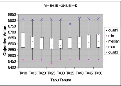
The objective values of these solutions were summarized using box plots. One

having |V| = 160, |E|= 2544 and |N| = 40. The box plot has the objective values on the

vertical axis and the tabu tenure values on the horizontal axis. The figure shows that the

range which spans the objective values of the best 50% of the solutions shifts downwards

with an increase in tabu tenure until T=25 and then moves upwards with further increase

in tabu tenure. This indicates an improvement in overall solution quality in the sense that,

on the whole, the objective values of the best 50% of the solutions decrease as the tabu

tenure increases until T=25, and the objective values increase with further increase in

tabu tenure, beyond T=25. If we use a similar argument considering the best 75% of the

solutions, then the best results are obtained at T=30.

Experimental runs conducted on various problem instances showed that the range of the

objective values of the top 50% solutions as well as the range of objective values for the

top 75% of the solutions were comparatively low for tabu tenure values lying between

|N|/2 and |N|, and the best ranges were also observed for some tabu tenure value lying

between |N|/2 and |N|. Thus, a dynamic tabu tenure was implemented. The tabu tenure

for each edge that becomes tabu is decided by generating a uniformly distributed random

Fig 2 Relating Solution quality with the tabu tenure

3.9.2 Number of iterations before diversification

The diversification procedure is intended to take the tabu search to an unexplored region

in the search space. The diversification takes place only if there is no improvement in the

best solution found for maxIterTillDiversify iterations. It is clear, that if the number of

iterations before diversification is too small then the neighborhood of a particular solution

will not be explored thoroughly. On the other hand, if the number of iterations is too

large, then a large amount of the solution space may remain unexplored by the time the

stopping criterion is satisfied.

|V| = 160, |E| = 2544, |N| = 40

8400

8450

8500

8550

8600

8650

8700

8750

8800

8850

Some sample runs of the tabu search were performed with the intention of obtaining

empirical evidence relating the quality of the solution to the parameter

maxIterTillDiversify, as was done with the tabu tenure parameter. The tabu search was

run with maxIterTillDiversify taking values between |N| and 5*|N| for several problem

sets, each

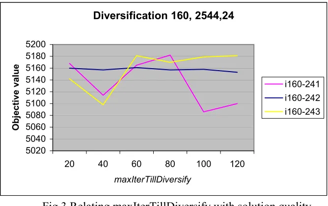
Fig 3 Relating maxIterTillDiversify with solution quality

set consisting of several instances, representing a particular problem size. The plot in Fig

3 is representative of the results obtained for the different problem sets. This plot

illustrates the results for one problem set containing three instances of same size (|V| =

160, |E| = 2544, |N| = 24). In the figure, the objective value obtained is plotted on the

vertical axis against the parameter maxIterTillDiversify on the horizontal axis. The three

lines represent three different problem instances, one line for each instance. As seen in

the Fig 3, the experimental runs do not indicate any obvious co-relation in the solution

quality with change in maxIterTillDiversify. Clearly, the observation makes the task of

selecting a value for this parameter somewhat difficult. A similar behavior was observed

in plots related to other problem sets. Hence, throughout the experiment we fix the value

Diversification 160, 2544,24

5020 5040 5060 5080 5100 5120 5140 5160 5180 5200

20 40 60 80 100 120

maxIterTillDiversify

Objective value

of maxIterTillDiversify at 4|N|, since this value seems to produce more good quality

solutions. Alternatively, instead of keeping the value of this parameter fixed, it can be

kept dynamic by assigning it uniformly distributed random values as the tabu search

proceeds.

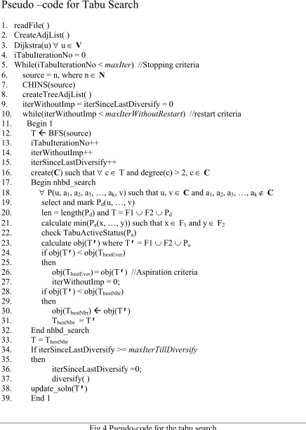
3.10 Pseudo-code for the Tabu search

A pseudo-code for the tabu search is given in Fig 4. Here we explain the code in more

detail. The tabu search algorithm begins by calling the function readfile() which reads the

test problem from the appropriate file containing the test problem. After reading the data

from the file, the function stores the graph as both an adjacency list as well as a weight

matrix. Next (in line 3) we run Dijkstra's single source shortest path algorithm from every

node in the graph, so as to obtain the shortest distance from any node to every other node

in the graph. From line 5, we begin the Tabu search by designating one of the terminal

nodes as a source node. The Tabu search runs for a fixed number of iterations which is

denoted by the parameter maxIter. Next we run the cheapest insertion method (a

constructive heuristic) to obtain the initial solution. This initial solution will be a tree

rooted at the source node. The initial solution available through CHINS() is in the form

of a parent array data structure. We use this parent array to create an adjacency list

structure for the initial steiner tree, in line 8. We now start the iterations of the Tabu

search that runs until no improved solutions are obtained during the search for

maxIterWithoutRestart iterations. This allows us to control the number of restarts. If we

maxIter. In line 12, we run the breadth first search algorithm on the current accepted

solution T. Next, in line 16, we create an array that contains all the critical nodes in T.

Beginning from line 17, we evaluate all the neighbors of T and select the best neighbor.

A neighbor of T is selected by identifying an unmarked key path Pd in T. We find the

length of Pd, mark it and then temporarily remove it from T to obtain two fragments F1

and F2. We find the shortest path that connects the two fragments F1 and F2 in line 21.

We ensure that the selected path is not Tabu Active and calculate the objective value of

the neighbor T' formed by connecting fragments F1 and F2 with the shortest path Pa. In

lines 24-27, we check whether Pa satisfies the aspiration criterion. If T' is better than the

best neighbor in the current neighborhood search then T' is stored as the best neighbor.

This ends the neighborhood search for T. If the total number of iterations without

improvement since the last diversification is greater than maxIterTillDiversify then we

apply the diversification procedure and obtain a T". Finally T' (or T") is made the

current solution and all relevant data structures are updated and the objective is

Pseudo –code for Tabu Search

1. readFile( ) 2. CreateAdjList( ) 3. Dijkstra(u) ∀ u ∈V

4. iTabuIterationNo = 0

5. While(iTabuIterationNo < maxIter) //Stopping criteria 6. source = n, where n ∈N

7. CHINS(source) 8. createTreeAdjList( )

9. iterWithoutImp = iterSinceLastDiversify = 0

10. while(iterWithoutImp < maxIterWithoutRestart) //restart criteria 11. Begin 1

12. T Å BFS(source)

13. iTabuIterationNo++

14. iterWithoutImp++

15. iterSinceLastDiversify++

16. create(C) such that ∀ c ∈ T and degree(c) > 2, c ∈C

17. Begin nhbd_search

18. ∀ P(u, a1, a2, a3, …, ak, v) such that u, v ∈C and a1, a2, a3, …, ak∉C

19. select and mark Pd(u, …, v)

20. len = length(Pd) and T = F1 ∪ F2 ∪ Pd

21. calculate min(Pa(x, …, y)) such that x ∈ F1 and y ∈ F2

22. check TabuActiveStatus(Pa)

23. calculate obj(T') where T' = F1 ∪ F2 ∪ Pa

24. if obj(T') < obj(TbestEver)

25. then

26. obj(TbestEver)=obj(T') //Aspiration criteria

27. iterWithoutImp = 0; 28. if obj(T') < obj(TbestNbr)

29. then

30. obj(TbestNbr) Å obj(T')

31. TbestNbr = T'

32. End nhbd_search

33. T = TbestNbr

34. If iterSinceLastDiversify >= maxIterTillDiversify

35. then

36. iterSinceLastDiversify =0;

37. diversify( )

38. update_soln(T')

39. End 1

4 Computational Experiments

In this chapter we present the results of computational experiments performed to evaluate

the effectiveness of the proposed algorithm on an empirical basis. Henceforth, we refer to

the tabu search algorithm that we have developed as TS. The experiments consist of

running TS on test problems of various sizes and comparing the objective values of the

solutions obtained to the known optimal values. The tabu search algorithm was also

compared to the best value obtained from all possible runs of the CHINS heuristic, which

is described in Section 2.2.1. The CHINS heuristic is applied repeatedly with each node

in the graph serving as the initial node. Thus, CHINS is run on each problem instance |V|

times and henceforth we will refer to the multiple runs of CHINS as the CHINS-V

heuristic. All programs for this algorithm were written in the C programming language

and were executed on a Sun Ultra 10 workstation.

4.1 Problem sets

The algorithm TS was tested on problem sets created by C. Duin [17]. These problem

instances for the steiner tree problem are of various sizes, types and difficulty and are

now available over the Internet. There are two important reasons for using these problem

sets. The first one is that these problems have been solved using some exact method such

as the branch and bound method described earlier and either the optimal value or an

upper bound on the optimal value for each problem is reported. The second important

edge exchange or node exchange procedures cannot be used to optimally solve these

instances.

The problem instances can be divided into two main sets based on the total number of

nodes in a particular instance. The first set contains instances of smaller size, each

containing 80 nodes. The second set has larger instances each having 160 nodes. Each of

these sets can be further broken down into subsets based on the edge density. Thus, each

set has problem instances having five different edge densities e = 3v/2, 2v, vlnv, 2vlnv,

v(v-1)/2 and 4 different terminal densities n = [log2v], [√v] , 2[log2v], [v/4], where e =

|E|, n = |N| and v = |V|. The source of the data also indicates the difficulty of the instance

in terms of the type of algorithm required to solve the problem and the order of

magnitude of time taken.

4.2 Performance measures

The tabu search algorithm is evaluated based on two performance measures. The first

measure compares the objective value of the solution obtained by TS for an instance to its

optimal value. This comparison is done with the help of the quantity ηopt which is defined

Thus, ηopt is the percentage difference between the tabu search value and the optimum

value for an instance. The second measure, ηCHINS-V, compares the objective value of the

solution obtained via TS with that of the best solution obtained by CHINS-V.

Thus,ηCHINS is the difference between the objective value obtained using the CHINS-V

heuristic and the tabu search value as a percentage of the optimum value for an instance.

4.3 Observations

All numerical results were obtained with the following parameter settings: tabu tenure

was a uniformly distributed random number between |N|/2 and |N|, the search was

stopped when no more nodes were available for the diversification procedure or when the

search had performed 5000 iterations. The diversification procedure was performed

whenever the search executed 4*|N| iterations without improvement in the best value

ηopt = CTS - Copt * 100

Copt

where Copt = optimum value

and CTS = objective value obtained by TS

ηCHINS = CCHINS – CTS * 100

Copt

where Copt = optimum value

CTS = objective value obtained using TS

obtained. Also, every 1000 iterations the search was restarted with a new initial solution

generated using the CHINS heuristic.

4.3.1 Comparison to Optimal Values

The problem instances are categorized into two sets based on the number of nodes |V|.

Let us refer to the problem set containing instances with 80 nodes as i080. Similarly i160

refers to the problem set containing instances having 160 nodes. The results for each set

are summarized in separate tables. The comparison of the TS solutions to the known

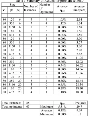
optimal values is displayed in Table 1 and Table 2. Table 1 contains results of the

problem instances from the set i080 and Table 2 contains results from the set i160. The

size of the problem is characterized by the number of nodes |V|, number of edges |E| and

the number of terminals |N|. There are at most 5 instances of the same size, i.e., instances

with the same values of |V|, |E| and |N|. Each row in Table 1 and Table 2 gives the

average value of ηopt and the average time per instance for all instances of the same size.

The tables also contain the total number of optimum solutions found by TS for each

problem size. At the end of each table we present a summary of the results for all

problem instances for that particular set.

For set i080, TS found the optimum value in 63 out of the 88 problem instances tested.

On the other hand for set i160, TS found the optimum in 46 out of the 94 instances. On

average, TS produced solutions, for set i080, which were within 0.38% of the optimal.

For set i160, TS came up with solutions that were within 0.54% of the optimal. The

reported in the tables is the total cpu time taken in seconds and includes the time required

to run Dijkstra’sall-source shortest path algorithm. The time required for the tabu search

algorithm increased with the problem size. Keeping the number of nodes constant, the

increase in time was more sensitive to an increase in the number of terminals than an

increase in the number of edges. This is to be expected, as the neighborhood search takes

up a large fraction of the time required for TS. Hence, the time required for TS increases

with neighborhood size. As we explained earlier in Section 3.3, the size of the

neighborhood is determined by the number of vertices in the solution T, more accurately,

the number of critical vertices in the solution. An increase in the number of terminals will

definitely lead to an increase in the number of critical vertices in the solution. On the

other hand, an increase in the number of edges (for the same |V| and |N|) may not lead to

an increase of the number of critical vertices in the solution.

The results for both sets i080 and i160 indicate that with an increase in the number of

terminals |N| there is a decrease in the number of optimal solutions found by TS. Also,

the deviation from the optimal value of solutions found by TS increases with an increase

in |N|. In many cases, TS finds the optimal in all but one instance. The deviation from the

optimal value for this instance may be as large as 5%. Moreover, in problem sets having

the same value of |V| and |N|, an increase in |E| does not increase the deviation from the

optimal. This indicates that the performance of the algorithm depends not only on the size

but also the structure of the instance. Thus, there seems to be a possibility that instances

with specific structure could be created for which TS would perform poorly as compared

Table 1 Summary of Results for problem set i080

Size |V| |E| |N|

Number of Instances Number of Optimums Average ηopt Average Time(secs) 80 120 6 5 4 1.05% 2.14 80 350 6 5 4 1.12% 1.34 80 3160 6 5 5 0.00% 1.68 80 160 6 5 5 0.00% 1.56 80 632 6 5 4 0.05% 1.56 80 120 8 3 3 0.00% 3.00 80 350 8 3 3 0.00% 3.27 80 3160 8 4 4 0.00% 3.00 80 160 8 4 4 0.00% 2.20 80 632 8 5 4 0.01% 2.62 80 120 16 4 4 0.00% 11.05 80 350 16 5 3 0.66% 12.02 80 3160 16 5 0 0.74% 16.02 80 160 16 5 5 0.00% 14.06 80 632 16 5 1 0.86% 11.86 80 120 20 2 2 0.00% - 80 350 20 5 4 0.36% 18.64 80 3160 20 5 0 0.65% 28.54 80 160 20 4 3 0.28% 18.30 80 632 20 4 1 1.18% 18.00

TS on Total Instances 88 ηopt Time(sec)

Table 2 Summary of Results for problem set i160

Size |V| |E| |N|

Total Instances No of Optimums Average ηCHINS-V Average Time(sec) 160 240 7 5 5 0.00% 11.00 160 812 7 5 5 0.00% 8.90 160 12720 7 5 4 0.04% 9.78 160 320 7 5 5 0.00% 8.83 160 2544 7 4 4 0.00% 8.53 160 240 12 3 2 1.96% 35.40 160 812 12 5 2 0.49% 30.00 160 12720 12 5 2 0.26% 28.48 160 320 12 5 5 0.00% 38.48 160 2544 12 5 2 0.58% 25.78 160 240 24 5 4 0.16% 155.06 160 812 24 5 1 0.66% 119.32 160 12720 24 5 0 0.73% 87.30 160 320 24 4 2 0.51% 125.95 160 2544 24 5 0 1.53% 100.72 160 240 40 5 3 0.20% 313.72 160 812 40 5 0 1.73% 293.40 160 12720 40 5 0 0.74% 179.32 160 320 40 5 0 0.34% 334.68 160 2544 40 3 0 1.77% 192.70

TS on Total Instances 94 ηCHINS-V Time

i160 Total optimums 46 Max 5.89% 375.2

4.3.2 Comparison of CHINS-V with TS

The heuristic that we refer to as CHINS-V in this section is the multiple pass version of

the CHINS heuristic that is described in Section 2.2.1. The heuristic is run |V| times

starting from a different node in every run. The CHINS-V heuristic is run on every

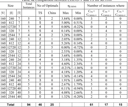
problem instance in the experiment. Tables 3a and 3b contain the comparison between

CHINS-V and TS for problem set i080, while the results for set i160 are in Tables 4a and

Table 4b.

As done in Table 1 and 2, the problem instances are grouped according to size and each

row contains the summary for instances of the same size. Firstly, TS and CHINS-V are

compared on the basis of the number of instances for which the optimal solution was

found by each method. The difference between the CHINS-V values and the TS values is

noted. Along with the number of optimums, Table 3a, for set i080, and Table 4a, for set

i160, show the maximum and the minimum values of the difference between CHINS-V

and TS for problem instances of the same size. The tables also indicate the number of

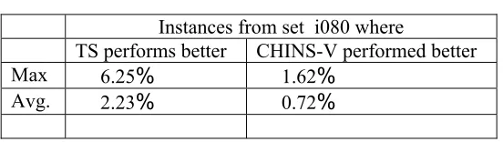
instances in which TS performed better, as good as, or worse than CHINS-V. Table 3b

displays a summary for all of the instances in i080. We divide the problem instances into

two groups. One group contains all the instances where TS outperformed CHINS-V and

the other contains all those instances where CHINS-V outperformed TS. The maximum

difference and the average difference between TS and CHINS-V for these two groups are

For the problem set i080, out of the 88 problem instances TS finds the optimal in 63

instances whereas CHINS-V finds the optimal in only 37 cases. With the exception of 3

problem sizes (all instances having same values of |E|, |V| and |N|), in all other problem

sizes TS outperforms CHINS-V. Altogether in set i080, TS is better in a total of 47

instances and on an average the difference is 2.23% of the optimum. On the other hand,

CHINS-V is better in only 12 instances and the average difference of 0.72% in these 11

instances is comparatively much less. The numbers for the set i160 indicate a similar

trend. In set i160, apart from three problem sizes, TS outperforms CHINS-V in all other

problem sizes. Out of the 94 instances tested, TS performs better in 61 with an average

improvement over CHINS-V of 2.25% while CHINS-V does better in only 15 instances

and with a comparatively lower average improvement over TS of 0.53%.

Thus for the 182 instances tested, the tabu search algorithm TS, obtains the optimal

solutions in 108 instances. On average, TS produces solutions within 0.46% of the

optimal value. Also, even though CHINS-V is much faster, TS produces better solutions

in most cases and in those cases where TS performs worse than CHINS-V, the average

Table 3a Comparison of CHINS-V with TS for set i080

Size No of Optimals ηCHINS Number of instances where

|V| |E| |N|

Total

Instances _{TS Chins Max Min} CTS <

CCHINS-V

CTS =

CCHINS-V

CTS >

CCHINS-V

80 120 6 5 4 3 0.17% -0.93% 1 3 1 80 350 6 5 4 1 0.34% 0.00% 3 2 0 80 3160 6 5 5 5 0.00% 0.00% 0 5 0 80 160 6 5 5 4 0.57% 0.00% 1 4 0 80 632 6 5 4 2 6.25% 0.00% 2 2 1 80 120 8 3 3 2 3.22% 0.00% 1 2 0 80 350 8 3 3 0 4.30% 0.11% 3 0 0 80 3160 8 4 4 4 0.00% 0.00% 0 4 0 80 160 8 4 4 3 4.42% 0.00% 1 3 0 80 632 8 5 4 3 3.30% 0.00% 1 4 0 80 120 16 4 4 0 2.34% 2.03% 4 0 0 80 350 16 5 3 0 4.27% 0.52% 5 0 0 80 3160 16 5 0 5 -0.06% -1.62% 0 0 5 80 160 16 5 5 0 4.57% 1.58% 5 0 0 80 632 16 5 1 0 4.17% 0.06% 5 0 0 80 120 20 2 2 0 3.45% 1.25% 2 0 0 80 350 20 5 4 0 3.88% 1.58% 5 0 0 80 3160 20 5 0 5 -0.43% -0.81% 0 0 5 80 160 20 4 3 0 3.37% 0.23% 4 0 0 80 632 20 4 1 0 2.81% 0.44% 4 0 0

Total 88 61 37 47 29 12

Table 3b Summary for set i080

Instances from set i080 where

TS performs better CHINS-V performed better Max 6.25% 1.62%

Table 4a Comparison between CHINS-V and TS for set i160

Size _InstancesTotal _{No of Optimals} ηCHINS Number of instances where

|V| |E| |T| TS Chins Max Min CTS <

CCHINS-V

CTS =

CCHINS-V

CTS >

CCHINS-V

160 240 7 5 5 2 3.84% 0.00% 3 2 0 160 812 7 5 5 0 5.00% 0.51% 5 0 0 160 12720 7 5 4 5 0.00% -0.22% 0 4 1 160 320 7 5 5 4 0.14% 0.00% 1 4 0 160 2544 7 4 4 2 3.28% 0.00% 2 2 0 160 240 12 3 2 1 2.05% 0.00% 2 1 0 160 812 12 4 2 0 5.26% 0.14% 4 0 0 160 12720 12 5 2 5 0.00% -0.72% 0 2 3 160 320 12 5 5 1 2.53% 0.00% 4 1 0 160 2544 12 5 2 0 3.68% 0.00% 4 1 0 160 240 24 5 4 0 3.18% 1.35% 5 0 0 160 812 24 5 1 0 4.60% 2.34% 5 0 0 160 12720 24 5 0 5 -0.21% -1.06% 0 0 5 160 320 24 4 2 0 4.18% 1.20% 4 0 0 160 2544 24 5 0 0 1.36% -0.14% 4 0 1 160 240 40 5 3 0 1.91% 1.60% 5 0 0 160 812 40 5 0 0 2.67% 1.79% 5 0 0 160 12720 40 5 0 0 0.11% -0.94% 1 0 4 160 320 40 5 0 0 4.08% 2.66% 5 0 0 160 2544 40 3 0 0 1.32% -0.20% 2 0 1

Total 94 46 25 61 17 15

Table 4b for set i160

Instances from set i160 where

TS performs better CHINS-V performed better Max 5.26% 1.06%

4.4 Concluding Remarks

To assess the efficiency of the proposed tabu search algorithm, it was applied to problem

sets specifically built for testing algorithms for the steiner tree problem [17]. The

algorithm was also compared with a multiple pass version of the CHINS heuristic. The

proposed tabu search algorithm produces optimal solutions in 59% of the instances

tested, and on average produces solutions within 0.46% of the optimal value. The tabu

search also performs better than or as good as CHINS-V in 85.2% of the instances and in

the 14.8% cases where it does worse than CHINS-V the difference in objective values, on