R E S E A R C H
Open Access
Chebyshev spectral collocation method for
stochastic delay differential equations
Zhengwei Yin
1,2and Siqing Gan
1**Correspondence:
1School of Mathematics and
Statistics, Central South University, Changsha, Hunan 410083, China Full list of author information is available at the end of the article
Abstract
The purpose of the paper is to propose the Chebyshev spectral collocation method to solve a certain type of stochastic delay differential equations. Based on a spectral collocation method, the scheme is constructed by applying the differentiation matrix
DNto approximate the differential operatordtd.DNis obtained by taking the derivative
of the interpolation polynomialPN(t), which is interpolated by choosing the first kind of Chebyshev-Gauss-Lobatto points. Finally, numerical experiments are reported to show the accuracy and effectiveness of the method.
Keywords: spectral collocation method; stochastic delay differential equations; Lamperti-type transformation; Chebyshev-Gauss-Lobatto nodes
1 Introduction
Deterministic differential models require that the parameters involved be completely known, though in the original problem, one often has insufficient information on param-eter values. These may fluctuate due to some external or internal ‘noise’, which is ran-dom. Thus, it is necessary to move from deterministic problems to stochastic problems. Stochastic differential equations (SDEs) play a prominent role in a range of application areas, such as biology, chemistry, epidemiology, mechanics, microelectronics, economics and so on [, ]. For SDEs, roughly speaking, there are two major types of numerical meth-ods, explicit numerical methods [, ] and implicit numerical methods [, ]. One can refer to [] for an overview of the numerical solution of SDEs.
In nature, there are many processes which involve time delays. That is, the future state of the system is dependent on some of the past history. Stochastic delay differential tions (SDDEs), which are a generalization of both deterministic delay differential equa-tions (DDEs) and stochastic ordinary differential equaequa-tions (SODEs), are better to simu-late these kinds of systems. In order to give the reader a general insight into the application of SDDEs, we introduce briefly the cell population growth model which is given as follows:
dx(t) = (ρx(t) +ρx(t–τ))dt+βdw(t), t≥,
x(t) =(t), –τ≤t< . (.)
Assume that these biological systems operate in a noisy environment whose overall noise rate is distributed like white noiseβdw(t). The constantτdenotes the average cell-division time. Then the populationx(t) is a random process, whose growth can be described by
(.). In fact, SDDEs as the stochastic models appear frequently in applied research and lead to an increasing interest in the investigation. For additional examples one can refer to applications in neural control mechanisms: neurological diseases [], human postural sway [] and pupil light reflex []. Since explicit solutions are rarely available for SDDEs, numerical approximations [, ] become increasingly important in many applications. To make the implementation viable, effective numerical methods are clearly the key ingre-dient and deserve much investigation. In the present work we make efforts in this direction and propose a new efficient scheme.
In the paper, we attempt to construct a Chebyshev spectral collocation method to solve SDDEs of the form
dx(t) =f(x(t),x(t–τ))dt+g(x(t))dw(t), t∈[,T],
x(t) =(t), t∈[–τ, ], (.)
where <T<∞andτis a positive fixed delay,f:R×R→Randg:R→Rare assumed to be continuous.w(t) is a one-dimensional standard Wiener process defined on the com-plete probability space (,Ft,P) with a filtration{Ft}t≥satisfying the usual conditions
(that is, it is increasing and right continuous whileFcontains allP-null sets).(t) is an
F-measurableC([–τ, ],R)-valued random process such thatE<∞(C([–τ, ],R)
is the Banach space of all continuous paths from [–τ, ]→Requipped with the supre-mum norm).
Our approach is derived by constructing the interpolating polynomial of degreeNbased on a spectral collocation method and applying the differentiation matrix to approximate the differential operator arising in SDDEs. The interpolating polynomial of degree Nis constructed by applying the Chebyshev-Gauss-Lobatto (C-G-L) points as interpolation points and the Lagrange polynomial as a trial function. To the best of our knowledge, they have not been utilized in solving SDDEs. Finally, we would like to mention that the idea of the spectral collocation was previously employed in [, ] to construct methods for SODEs and DDEs. The authors in [] propose a spectral collocation method for SODEs. Inspired by the idea, we construct the Chebyshev spectral collocation method for SDDEs. This paper is organized as follows. In the next section, some fundamental knowledge is reviewed and the derivation of the Chebyshev spectral collocation for solving SDDEs is introduced. Section is devoted to reporting some numerical experiments to confirm the accuracy and effectiveness of the method. At the end of the article, conclusions are made briefly.
2 Construction of the Chebyshev spectral collocation method 2.1 The Lamperti-type transformation
In this section, we introduce the Lamperti-type transformation [], which can guarantee that the diffusion term of (.) is a constant. For equation (.), assume
y(t) =Fx(t)= x(t)
u
where uis any arbitrary value in the state space of X. For ≤t≤T, applying the Itô formula yields
dy(t) =
f(x(t),x(t–τ)) g(x(t)) –
g
x(t)dt+dw(t)
=
f(F–(y(t)),F–(y(t–τ))) g(F–(y(t))) –
g
F–y(t)dt+dw(t). (.)
Let
by(t),y(t–τ)=f(F
–(y(t)),F–(y(t–τ)))
g(F–(y(t))) –
g
F–y(t). (.)
Hence, equation (.) can be rewritten simply as
dy(t) =by(t),y(t–τ)dt+dw(t), ≤t≤T. (.)
Using the Lamperti transform, one can transform equation (.) into (.). Therefore, here and hereafter, we only consider the SDDEs of the form
dx(t) =b(x(t),x(t–τ))dt+dw(t), t∈[,T],
x(t) =(t), t∈[–τ, ]. (.)
2.2 Review on Chebyshev interpolation polynomials
Chebyshev polynomials are a well-known family of orthogonal polynomials on the interval [–, ]. These polynomials present, among others, very good properties in the approxima-tion of funcapproxima-tions. Therefore, Chebyshev polynomials appear frequently in several fields of mathematics, physics and engineering. In this subsection, we will recall the Chebyshev interpolation polynomial for a given functionx(t)∈Ck(–, ), whereCkis the space of all functions whosektimes derivatives are continuous on the interval (–, ). More details can be found in [].
Let Tk(t) =cos(karccos(t)) be the first kind Chebyshev polynomial of degree k and chooseN+ Chebyshev-Gauss-Lobatto (C-G-L) nodes such that
tj=cos
(N–j)π
N , j= , , . . . ,N. (.)
Define the Lagrange basis functions as follows:
lk(t) =
ω(t) (t–tk)ω(tk)
, k= , , . . . ,N, (.)
whereω(t) is given by
ω(t) = (t–t)(t–t)· · ·(t–tN).
It is noted that for k,j= , , . . . ,N the Lagrange interpolating basis functions have the Kronecker property
lk(tj) =
To sum up, the Chebyshev interpolation polynomial for a functionx(t) can be given by
Define the differentiation matrix by
DN=
Remark . The differentiation matrixDN is not dependent on the problem itself but
dependent on the C-G-L nodes. Therefore, the differentiation matrices can be obtained before a problem setting.
Remark . Differentiation matrices are derived from the spectral collocation method
for solving differential equations of boundary value type, more details can be found in [, ].
Remark .([]) The differentiation matrixDN itself is singular.
2.3 Chebyshev spectral collocation method for DDEs
Spectral method is one of the three technologies for numerical solutions of partial dif-ferential equations. The other two are finite difference methods (FDMs) and finite ele-ment methods (FEMs). The spectral methods based on Chebyshev polynomials as basis functions for solving numerical differential equations [–] with smooth coefficients and simple domain have been well applied by many authors. Furthermore, they can often achieve ten digits of accuracy while FDMs and FEMs would get two or three. An inter-ested reader can refer to references [, ]. Later, the spectral methods are developed to solve neutral differential equations [] or special DDEs []. In this subsection, we will introduce the spectral collocation method for DDEs.
Consider the DDEs
dx(t) =f(x(t),x(t–τ))dt, t∈[,T],
Lett=T( +s),x(t) =x(T( +s)) :=y(s), one can transform equation (.) into the
follow-T – , –]. Using the transformation, we shift the interval of the solution of DDEs (.) from [,T] into [–, ]. Therefore, in the following we focus mainly on the DDEs as follows:
dx(t) =f(x(t),x(t–τ))dt, t∈[–, ],
x(t) =ϕ(t), t∈[–τ– , –]. (.)
Approximating the functionx(t) on the left-hand side of (.) by the interpolation poly-nomialPN(t) defined in (.) yields replacing the differential operator dtd with the differentiation matrixDN, one can obtain
DNX=
one can obtain the discrete approximative equations for DDEs (.)
DNX=F. (.)
It is appropriate to emphasize that the remainder elements of the vectorX= (x,x, . . . ,
xN)T are unknown except the first elementxwhich can be calculated by the condition
take a transformy(t) =x(t) –xto vanish the initial condition. Subsequently, we give an
Remark . Note thatxis fixed at zero in the approximative equation (.). This implies
that the first column ofDNhas no effect (since multiplied by zero) and the first row has no effect either (since ignored). Therefore, by removing the first row and first column ofDN, we can get a new matrix denoted by
˜
Remark . By removing the first row and the first column ofAand the first element of the vectorsX,drespectively, one can get
˜ the discrete approximative (.).
2.4 The Chebyshev spectral collocation method for SDDEs
In this subsection, we first give the theorem to guarantee the existence and uniqueness of the exact solution of SDDE (.).
Theorem .([, ]) Assume that there exist positive constants Lf,i,i= , ,and Kf such that both the functions f and g satisfy a uniform Lipschitz condition and a linear growth bound of the following form,for allζ,ζ,η,η,ζ,η∈Rand t∈[,T]:
f(ζ,η) –f(ζ,η)≤Lf,|ζ–ζ|+Lf,|η–η|,
f(ζ,η)≤Kf
+|ζ|+|η|,
and likewise for g with constants Lg and Kg.Then there exists a path-wise unique strong solution to(.).
Consider the SDDEs
dx(t) = (f(x(t),x(t–τ)))dt+dw(t), t≥,
x(t) =ϕ(t), t∈[–τ, ]. (.)
solution. Equation (.) is transformed from (.) by using the Lamperti-type transfor-mation. Hence, there exists a path-wise unique strong solution to (.). Following the same lines as mentioned in Section ., it is easy to obtain the approximative equations for SDDE (.) as follows:
˜
DNX˜=g(X˜,A˜X˜ +d˜) +D˜Nw, (.)
where theN-dimensional vectorg(X˜,A˜X˜+d˜) has the componentsgi=f(xi,ϕ(ti–τ)) fori= , . . . ,mandgi=f(xi,
N
k=xklk(ti–τ)) fori=m+ , . . . ,N. Applying the invertible property of the matrix yields
˜ X=D˜–
Ng(X˜,A˜X˜+d˜) +w. (.)
Remark . To find the derivative of functionx(t) on C-G-L nodes,DNxis of high ac-curacy only ifx(t) is smooth enough. But the standard Wiener processw(t) is a nowhere differentiable process, DNwbehaves very badly. However, if the coefficient of diffusion term of SDDEs is a constant, we can avoidDNwas above (see []).
3 Numerical experiments
The theoretical discussion of numerical processes is intended to provide an insight into the performance of numerical methods in practice. Therefore, in this section, some nu-merical experiments are reported to test the accuracy and the effectiveness of the spectral collocation method.
Example Consider the SDDE
dx(t) =ax(t) +bx(t– )dt+β+βx(t) +βx(t– )
dw(t) (.)
as a test equation for our method. In the case of additive noise (β=β= ), an explicit
solution on the first interval [,τ] has been calculated by the method of steps (see, for example, []). Usingϕ(t) = +tfort∈[–, ] as an initial function, the solution ont∈ [, ] is given by
x(t) =eat
+ b a
–b
at– b a +βe
at t
e–asdw(s). (.)
In our experiments, the mean-square errorE(|x(T) –X¯N|) (note thatX¯Nis the last ele-ment of the vectorX˜Ncalculated by (.)) at the final timeTis estimated in the following way. A set of blocks, each containing outcomes (ωi,j, ≤i≤, ≤j≤), is sim-ulated, and for each block the estimator
i=
j=
x(T,ωi,j) –X¯N(ωi,j)
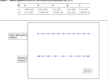
Table 1 Mean-square errors of the numerical solutions for (3.1)
N 3 4 5 6 7
I 4.38e–002 3.24e–002 5.7e–003 5.5e–003 9.1e–003
II 3.1e–003 1.7349e–05 5.5209e–06 5.6e–003 2.2626e–05
Figure 1 An explanation of collocation points for the Euler-Maruyama method and the spectral collocation method on a subinterval.
It is noted that, for the Chebyshev spectral method, we collocateN+ points on the interval. Hence, there existNsubintervals. Different from the Euler-Maruyama method [] for solving SDDEs, the subintervals are not equidistant, and the distance between suc-cessive Chebyshev points is
√
–x
N ,x∈[–, ]. Figure [] shows the difference between the two methods.
We apply the spectral collocation method to solve (.) under the set of coefficients I: a= –.,b= .,β= . and II:a= –,b= .,β= . The numerical results are shown in
Table . In Table , we denoteNby the number of the C-G-L nodes. The approximation errors reported in Table show that the Chebyshev spectral collocation method works very well for SDDEs and has high accuracy and effectiveness.
Example Consider (.) as a DDE,i.e.,β=β=β= , which reads
dx(t) = (a(x(t) +bx(t– )))dt, t> ,
x(t) = +t, –≤t≤. (.)
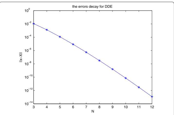
We apply the spectral collocation method for (.) with two groups of parameters I:a= –.,b= and II:a= –,b= .. In Tables and , for (.) with the parameters I and II, we list the approximation errors of the spectral collocation methods with differentNwhich is denoted by the number of the C-G-L nodes. It is clear that the spectral accuracy and the convergence are obtained when the spectral collocation method is applied to solve (.).
Fig-Table 2 Errors for equation (3.3) in the case ofa= –0.9,b= 1
N x – XL∞(0,1)
3 2.3e–003
4 1.082e–004
5 4.169e–006
6 1.356e–007
7 3.831e–009
N x – XL∞(0,1)
8 9.597e–011
9 2.160e–012
10 4.430e–014
11 6.661e–016
12 4.441e–016
Table 3 Errors for equation (3.3) in the case ofa= –2,b= 0.1
N x – XL∞(0,1)
3 1.10e–002
4 1.3e–003
5 1.160e–004
6 8.647e–006
7 5.543e–007
N x – XL∞(0,1)
8 3.129e–8
9 1.581e–009
10 7.242e–011
11 3.034e–012
12 1.170e–013
Figure 2 The error decay for equation (3.3) in the case ofa= –0.9,b= 1.
ures and . As one may expect, the errors decay very quickly with the increase in the number of the interpolation points.
4 Conclusions
Figure 3 The error decay for equation (3.3) in the case ofa= –2,b= 0.1.
Competing interests
The authors declare that they have no competing interests.
Authors’ contributions
Both authors contributed equally to the writing of this paper. Both authors read and approved the final manuscript.
Author details
1School of Mathematics and Statistics, Central South University, Changsha, Hunan 410083, China.2School of
Mathematics and Statistics, Henan University of Science and Technology, Luoyang, Henan 410083, China.
Acknowledgements
The authors would like to thank the anonymous referees for their valuable and insightful comments which have improved the paper. This work is supported by the National Natural Science Foundation of China (No. 11171352, No. 11301550), the New Teachers’ Specialized Research Fund for the Doctoral Program from the Ministry of Education of China (No. 20120162120096) and Mathematics and Interdisciplinary Sciences Project, Central South University.
Received: 10 December 2014 Accepted: 19 March 2015
References
1. Bodo, BA, Thompson, ME, Labrie, C, Unny, TE: A review on stochastic differential equations for application in hydrology. Stoch. Hydrol. Hydraul.1(2), 81-100 (1987)
2. Wilkinson, DJ, Platen, E, Schurz, H: Stochastic modelling for quantitative description of heterogeneous biological systems. Nat. Rev. Genet.10, 122-133 (2009)
3. Maruyama, G: Continuous Markov processes and stochastic equations. Rend. Circ. Mat. Palermo4(1), 48-90 (1955) 4. Milstein, GN: Approximate integration of stochastic differential equations. Theory Probab. Appl.19(3), 557-562 (1975) 5. Kloeden, PE, Platen, E, Schurz, H: The numerical solution of nonlinear stochastic dynamical systems: a brief
introduction. Int. J. Bifurc. Chaos1(2), 277-286 (1991)
6. Milstein, GN, Platen, E, Schurz, H: Balanced implicit methods for stiff stochastic systems. SIAM J. Numer. Anal.35(3), 1010-1019 (1998)
7. Kloeden, PE, Platen, E: Numerical Solution of Stochastic Differential Equations. Springer, Berlin (1992) 8. Beuter, A, Bélair, J, Labrie, C: Feedback and delays in neurological diseases: a modelling study using dynamical
systems. Bull. Math. Biol.55(3), 525-541 (1993)
9. Eurich, CW, Milton, JG: Noise-induced transitions in human postural sway. Phys. Rev. E54, 6681-6684 (1996) 10. Mackey, MC, Longtin, A, Milton, JG, Bos, JE: Noise and critical behaviour of the pupil light reflex at oscillation onset.
Phys. Rev. A41, 6992-7005 (1990)
11. Buckwar, E: Introduction to the numerical analysis of stochastic delay differential equations. J. Comput. Appl. Math. 125, 297-307 (2000)
12. Christopher, THB, Buckwar, E, Labrie, C, Unny, TE: Numerical analysis of explicit one-step method for stochastic delay differential equations. LMS J. Comput. Math.3, 315-335 (2000)
14. Wang, W, Li, D: Convergence of spectral method of linear variable coefficient neutral differential equation with variable delays. Math. Numer. Sin.34(1), 68-80 (2012)
15. Lacus, SM, Platen, E: Simulation and Inference for Stochastic Differential Equations. Springer, Berlin (2007)
16. Elbarbary, EME, El-Kady, M: Chebyshev finite difference approximation for the boundary value problems. Appl. Math. Comput.139(2-3), 513-523 (2003)
17. Ibrahim, MAK, Temsah, RS: Spectral methods for some singularly perturbed problems with initial and boundary layers. Int. J. Comput. Math.25(1), 33-48 (1988)
18. Ali, I: A spectral method for pantograph-type delay differential equations and its convergence analysis. Appl. Comput. Math.27(2-3), 254-265 (2009)
19. Canuto, C, Hussaini, MY, Quarteroni, A, Zang, TA: Spectral Methods Fundamentals in Single Domains. Springer, Berlin (2006)
20. She, J, Tang, T: Spectral and High-Order Methods with Applications. Science Press, Beijing (2006)
21. Mizel, VJ, Trutzer, V: Stochastic hereditary equations: existence and asymptotic stability. J. Integral Equ.7, 1-72 (1984) 22. Mao, X: Stochastic Differential Equations and Their Applications. Ellis Horwood, Chichester (1997)