HYBRID SOFT COMPUTING: THE PERCEPTION

22 | P a g e

HYBRID SOFT COMPUTING: THE PERCEPTION

Santosh G Kondaguli

, Basavaraj M Hunshal

1,2

Department of CSE, KLE CET, Chikodi, Karnataka, (India)

ABSTRACT

Soft computing is the usage of inexact solutions to compute hard tasks for which there is no known algorithm

that can compute an exact solution in polynomial time. The soft computing solutions are unpredictable. Hybrid

soft computing is an association of computing methodologies that includes fuzzy logic, neuro-computing,

evolutionary computing and probabilistic computing. After a brief overview of Soft Computing components, we

analyzed the Artificial Neuro Fuzzy Interface System. We also emphasize the development of smart

algorithm-controllers, such as the use of fuzzy logic to control the parameters of evolutionary computing and, conversely,

the application of evolutionary algorithms to tune fuzzy controllers.

Keywords

:

Computing, Probabilistic Computing

I

INTRODUCTION

There is a wide scope of industrial and commercial problems that require the analysis of uncertain and imprecise

information. Usually, an incomplete understanding of the problem domain further compounds the problem of

generating models used to explain past behaviors or predict future ones. These problems present a great

opportunity for the application of soft computing technologies. In the industrial world, it is increasingly

common for companies to provide diagnostics and prognostics services for expensive machinery (e.g.,

locomotives, aircraft engines, medical equipment). Many manufacturing companies are trying to shift their

operations to the service field where they expect to find higher margins. Since performing unnecessary

maintenance actions is undesired and costly, in the interest of maximizing the margins, service should only be

performed when required. This can be accomplished by using a tool that measures the state of the system and

indicates any incipient failures. Such a tool must have a high level of sophistication that incorporates

monitoring, fault detection, decision making about possible preventive or corrective action, and monitoring of

its execution. A second industrial challenge is to provide intelligent automated controllers for complex dynamic

systems that are currently controlled by human operators.

For instance automatic freight train handling is a task that still eludes full automation.

Soft computing was first proposed by Zadeh [4] to construct new generation computationally intelligent hybrid

systems consisting of neural networks, fuzzy inference system, approximate reasoning and derivative free

optimization techniques. It is well known that the intelligent systems, which can provide human like expertise

such as domain knowledge, uncertain reasoning, and adaptation to a noisy and time varying environment, are

important in tackling practical computing problems. In contrast with conventional AI techniques (hard

computing), which only deal with precision, certainty and rigor the guiding principle of soft computing is to

23 | P a g e

includes as its principal members fuzzy logic (FL), neuro-computing (NC), evolutionary computing (EC) and

probabilistic computing (PC)” [5].

The main reason for the popularity of soft computing is the synergy derived from its components. SC’s main

characteristic is its intrinsic capability to create hybrid systems that are based on a (loose or tight) integration of

constituent technologies. This integration provides complementary reasoning and searching methods that allow

us to combine domain knowledge and empirical data to develop flexible computing tools and solve complex

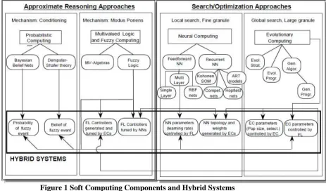
problems. Figure 1 illustrates a taxonomy of these hybrid algorithms and their components. Extensive coverage

of this topic can be found in [7, 8].

II

SOFT

COMPUTING

AND

CLASSIFICATION

2.1

Fuzzy Computing

The treatment of imprecision and vagueness can be traced back to the work of Post, Kleene, and Lukasiewicz,

multiple-valued logicians who in the early 1930's proposed the use of three-valued logic systems (later followed

by infinite-valued logic) to represent undetermined, unknown, or other possible intermediate truth-values

between the classical Boolean true and false values [9]. In 1937, the philosopher Max Black suggested the use

of a consistency profile to represent vague concepts [10]. While vagueness relates to ambiguity, fuzziness

addresses the lack of sharp set-boundaries. In a narrow sense, fuzzy logic could be considered a fuzzification of

Lukasiewicz Aleph-1 multiple-valued logic [12].

Figure 1 Soft Computing Components and Hybrid Systems

In the broader sense, however, this narrow interpretation represents only one of FL’s four facets [13]. More

24 | P a g e

representation and use of fuzzy relations;and an epistemic facet, covering the use of FL to fuzzy knowledge

based systems and data bases. A comprehensive review of fuzzy logic and fuzzy computing can be found in

[14]. Fuzzy logic gives us a language, with syntax and local semantics, in which we can translate qualitative

knowledge about the problem to be solved. In particular, FL allows us to use linguistic variables to model

dynamic systems. These variables take fuzzy values that are characterized by a label (a sentence generated from

the syntax) and a meaning (a membership function determined by a local semantic procedure). The meaning of a

linguistic variable may be interpreted as an elastic constraint on its value.

Philosopher Max Black suggested the use of a consistency profile to represent vague concepts [10]. While

vagueness relates to ambiguity, fuzziness addresses the lack of sharp set-boundaries. It was not until 1965, when

Zadeh proposed a complete theory of fuzzy sets (and its isomorphic fuzzy logic), that we were able to represent

and manipulate illdefined concepts [11].

Fuzzy logic could be considered a fuzzification of Lukasiewicz Aleph-1 multiple-valued logic [12]. In the

broader sense, however, this narrow interpretation represents only one of FL’s four facets [13].

More specifically, FL has a logical facet, derived from its multiple-valued logic genealogy; a set-theoretic facet,

stemming from the representation of sets with ill-defined boundaries; a relational facet, focused on the

representation and use of fuzzy relations; and an epistemic facet, covering the use of FL to fuzzy knowledge

based systems and databases. A comprehensive review of fuzzy logic and fuzzy computing can be found in [14].

Fuzzy logic gives us a language, with syntax and local semantics, in which we can translate qualitative

knowledge about the problem to be solved. In particular, FL allows us to use linguistic variables to model

dynamic systems. These variables take fuzzy values that are characterized by a label (a sentence generated from

the syntax) and a meaning (a membership function determined by a local semantic procedure). The meaning of a

linguistic variable may be interpreted as an elastic constraint on its value. These constraints are propagated by

fuzzy inference operations, based on the generalized modus-ponens. This reasoning mechanism, with its

interpolation properties, gives FL robustness with respect to variations in the system's parameters, disturbances,

etc., which is one of FL's main characteristics [15].

2.2

Probabilistic Computing

Rather than retracing the history of probability, we will focus on the development of probabilistic computing

(PC) and illustrate the way it complements fuzzy computing. As depicted in Figure 1, we can divide

probabilistic computing into two classes: single-valued and interval-valued systems. Bayesian belief networks

(BBNs), based on the original work of Bayes [16], is a typical example of single-valued probabilistic reasoning

systems. They started with approximate methods used in first-generation expert systems, such as MYCIN’s

confirmation theory [17] and PROSPECTOR’s modified Bayesian rule [18], and evolved into formal methods

for propagating probability values over networks [19-20]. In general, probabilistic reasoning systems have

exponential complexity, when we need to compute the joint probability distributions for all the variables used in

a model. Before the advent of BBNs, it was customary to avoid such computational problems by making

25 | P a g e

between two variables is indicated by the presence or lack of a link connecting the nodes representing such

variables in the network topology. For specialized topologies (trees, poly-trees, directed acyclic graphs),

efficient propagation algorithms have been proposed by Kim and Pearl [21]. However, the complexity of

multiple–connected BBNs is still exponential in the number of nodes of the largest sub-graph. When graph

decomposition is not possible, we resort to approximate methods, such as clustering and bounding conditioning,

and simulation techniques, such as logic samplings and Markov simulations.

Dempster-Shafer (DS) systems are a typical example of interval-valued probabilistic reasoning systems. They

provide lower and upper probability bounds instead of a single value as in most BBN cases. The DS theory was

developed independently by Dempster [22] and Shafer [23]. Dempster proposed a calculus for dealing with

interval-valued probabilities induced by multiple-valued mappings. Shafer, on the other hand, started from an

axiomatic approach and defined a calculus of belief functions. His purpose was to compute the credibility

(degree of belief) of statements made by different sources, taking into account the sources’ reliability. Although

they started from different semantics, both calculi were identical.

Probabilistic computing provides a way to evaluate the outcome of systems affected by randomness (or other

types of probabilistic uncertainty). PC’s basic inferential mechanism - conditioning - allows us to modify

previous estimates of the system's outcome based on new evidence.

Comparison between Probabilistic and Fuzzy Computing

In this brief review of fuzzy and probabilistic computing, we would like to emphasize that randomness and

fuzziness capture two different types of uncertainty. In randomness, the uncertainty is derived from the

nondeterministic membership of a point from a sample space (describing the set of possible values for the

random variable), into a well-defined region of that space (describing the event). A probability value describes

the tendency or frequency with which the random variable takes values inside the region. In fuzziness, the

uncertainty is derived from the deterministic but partial membership of a point (from a reference space) into an

imprecisely defined region of that space. The region is represented by a fuzzy set. The characteristic function of

the fuzzy set maps every point from such space into the real-valued interval [0, 1], instead of the set {0,1}. A

partial membership value does not represent a frequency. Rather, it describes the degree to which that particular

element of the universe of discourse satisfies the property that characterizes the fuzzy set. In 1968, Zadeh noted

the complementary nature of these two concepts, when he introduced the probability measure of a fuzzy event

[24]. In 1981, Smets extended the theory of belief functions to fuzzy sets by defining the belief of a fuzzy event

[25]. These are the first two cases of hybrid systems illustrated in Figure 1.

2.3

Neural Computing

The genealogy of neural networks (NN) goes back to 1943, when McCulloch and Pitts showed that a network of

binary decision units (BDNs) could implement any logical function [26]. Building upon this concept, Rosenblatt

proposed a one-layer feed-forward network, called a perceptrons, and demonstrated that it could be trained to

classify patterns [27-29]. Minsky and Papert [30] proved that single-layer perceptrons could only provide linear

26 | P a g e

these limitations. The training of these networks, however, was still problematic. Finally, the introduction of

back-propagation (BP), independently developed by Werbos [31], Parker [32], and LeCun [33], provided a

sound theoretical way to train multi-layered, feed-forward networks with nonlinear activation functions. In

1989, Hornik et al. proved that a three-layer NN (with one input layer, one hidden layer of squashing units, and

one output layer of linear units) was a universal functional approximator [34].

Topologically, NNs are divided into feed-forward and recurrent networks. The feed-forward networks include

single- and multiple-layer perceptrons, as well as radial basis functions (RBF) networks [35]. The recurrent

networks cover competitive networks, self-organizing maps (SOMs) [36], Hopfield nets [37], and adaptive

resonance theory (ART) models [38]. While feed-forward NNs are used in supervised mode, recurrent NNs are

typically geared toward unsupervised learning, associative memory, and self-organization. In the context of this

paper, we will only consider feed-forward NNs. Given the functional equivalence already proven between RBF

and fuzzy systems [39] we will further limit our discussion to multilayer feed-forward networks. A

comprehensive current review of neuro-computing can be found in [40]. Feed-forward multilayer NNs are

computational structures that can be trained to learn patterns from examples. They are composed of a network of

processing units or neurons. Each neuron performs a weighted sum of its input, using the resulting sum as the

argument of a nonlinear activation function. Originally the activation functions were sharp thresholds (or

Heavyside) functions, which evolved to piecewise linear saturation functions, to differentiable saturation

functions (or sigmoids), and to Gaussian functions (for RBFs). By using a training set that samples the relation

between inputs and outputs, and a learning method that trains their weight vector to minimize a quadratic error

function, neural networks offer the capabilities of a supervised learning algorithm that performs fine-granule

local optimization.

2.4

Evolutionary Computing

Evolutionary computing (EC) algorithms exhibit an adaptive behavior that allows them to handle non-linear,

high dimensional problems without requiring differentiability or explicit knowledge of the problem structure. As

a result, these algorithms are very robust to time-varying behavior, even though they may exhibit low speed of

convergence. EC covers many important families of stochastic algorithms, including evolutionary strategies

(ES), proposed by Rechenberg [41] and Schwefel [42], evolutionary programming (EP), introduced by Fogel

[43-44], and genetic algorithms (GAs), based on the work of Fraser [45], Bremermann [46], Reed et al. [47],

and Holland [48-50], which contain as a subset genetic programming (GP), introduced by Koza [51].

The history of EC is too complex to be completely summarized in a few paragraphs. It could be traced back to

Friedberg [52], who studied the evolution of a learning machine capable of computing a given input-output

function; Fraser [45] and Bremermann [46], who investigated some concepts of genetic algorithms using a

binary encoding of the genotype; Barricelli [53], who performed some numerical simulation of evolutionary

processes; and Reed et al. [47], who explored similar concepts in a simplified poker game simulation. The

interested reader is referred to [54] for a comprehensive overview of evolutionary computing and to [55] for an

encyclopedic treatment of the same subject. A collection of selected papers illustrating the history of EC can be

27 | P a g e

originally proposed for the optimization of continuous parameter spaces. In typical ES notation the symbols

(,)-ES and (+)-ES indicate the algorithms in which a population of parents generate offspring; the best

individuals are selected and kept in the next generation.

In the case of (,)-ES the parents are excluded from the selection and cannot be part of the next generation,

while in the (+)-ES they can. In their early versions, ES used a continuous representation and mutation

operator working on a single individual to create a new individual, i.e., (+)-ES. Later, a recombination

operator was added to the mutation operator as evolution strategies were extended to evolve a population of

individuals, as in (+1)-ES [57] and in (+)-ES [58]. Each individual has the same opportunity to generate an

offspring. Furthermore, each individual has its own mutation operator, which is inherited and may be different

for each parameter. In its early versions, evolutionary programming was applied to identification, sequence

prediction, automatic control, pattern recognition, and optimal gaming strategies [43]. To achieve these goals,

EP evolved finite state machines that tried to maximize a payoff function.

However, recent versions of EP have focused on continuous parameter optimization and the training of neural

networks [59]. As a result, EP has become more similar to ES. The main distinction between evolutionary

programming and evolutionary strategies is that EP focuses on the behavior of species, while ES focus on the

behavior of individuals. Therefore, EP does not usually employ crossover as a form of variation operator. EP

can be considered as a special case of (+)-ES, in which mutation is the only operator used to search for new

solutions.

Genetic algorithms perform a randomized global search in a solution space by using a genotypic rather than

phenotypic representation. Canonical GAs encode each candidate solution to a given problem as a binary,

integer, or real-valued string, referred to as chromosome. Each string's element represents a particular feature in

the solution. The string is evaluated by a fitness function to determine the solution's quality: better-fit solutions

survive and produce offspring, while less-fit solutions are gathered from the population. To evolve current

solutions, each string can be modified by two operators: crossover and mutation. Crossover acts to capture the

best features of two parents and pass it to an offspring. Mutation is a probabilistic operator that tries to introduce

needed features in populations of solutions that lack such features. The new individuals created by these

operators form the next generation of potential solutions. The problem constraints are typically modeled by

penalties in the fitness function or encoded directly in the solution data structures [60].

Genetic programming is a particular form of GA, in which the chromosome has a hierarchical rather than a

linear structure whose size is not predefined. The individuals in the population are tree structured programs, and

the genetic operators are applied to their branches (subtrees) or to single nodes. This type of chromosome can

represent the parse tree of an executable expression, such as an S-expression in LISP, an arithmetic expression,

etc. GP has been used in time-series predictions, control, optimization of neural network topologies, etc. EC

components have increasingly shared their typical traits: ES have added recombination operators similar to GAs,

while GAs have been extended by the use of real-number-encoded chromosomes, adaptive mutation rates, and

additive mutation operators. For the sake of brevity, in the context of this paper, we will limit most of our

28 | P a g e

III

ARTIFICIAL

NEURAL

NETWORKS

Artificial Neural Networks (ANNs) have been developed as generalizations of mathematical models of

biological nervous systems. A neural network is characterized by the network architecture, the connection

strength between pairs of neurons (weights), node properties, and updating rules.

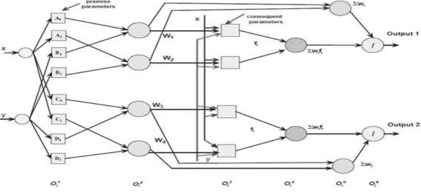
Figure 2 Architecture of ANFIS with multiple output

The updating or learning rules control weights and/or states of the processing elements (neurons). Normally, an

objective function is defined that represents the complete status of the network, and its set of minima

corresponds to different stable states of the network. It can learn by adapting its weights to changes in the

surrounding environment, can handle imprecise information, and generalize from known tasks to unknown ones.

Back-propagation is a gradient descent technique to minimize some error criteria E. A good choice of several

parameters (initial weights, learning rate, momentum etc.) is required for training success and speed of the

ANN. Empirical research has shown that back-propagation algorithm often is stuck in a local minimum mainly

because of the random initialization of weights. Back-propagation usually generalizes quite well to detect the

global features of the input but after prolonged training the network will start to recognize individual

input/output pair rather than settling for weights that generally describe the mapping for the whole training set.

In the Conjugate Gradient Algorithm (CGA) a search is performed along conjugate directions, which produces

generally faster convergence than steepest descent directions. A search is made along the conjugate gradient

direction to determine the step size, which will minimize the performance function along that line. A line search

is performed to determine the optimal distance to move along the current search direction. Then the next search

direction is determined so that it is conjugate to previous search direction. The general procedure for

determining the new search direction is to combine the new steepest descent direction with the previous search

direction. An important feature of the CGA is that the minimization performed in one step is not partially

undone by the next, as it is the case with gradient descent methods. An important drawback of CGA is the

requirement of a line search, which is computationally expensive. Moller introduced the Scaled Conjugate

29 | P a g e

model forex monitoring systems.

3.1

Neuro-fuzzy Computing

Neuro-Fuzzy (NF) computing is a popular framework for solving complex problems [61]. We used the Adaptive

Neuro Fuzzy Inference System (ANFIS) implementing a multi-output Takagi-Sugeno type Fuzzy Inference

System (FIS) [62]. Figure 2 depicts the 6- layered architecture of multiple output ANFIS.

The detailed function of each layer is as follows:

Layer-1: Each node in this layer corresponds to one linguistic label (excellent, good, etc.) to one of the input

variables in the input layer (x,..,y). In other words, the output link represent the membership value, which

specifies the degree to which an input value belongs to a fuzzy set, is calculated in this layer. A clustering

algorithm (usually the grid partitioning method) will decide the initial number and type of membership functions

to be allocated to each of the input variable. The

final shapes of the MFs will be ¯ne tuned during network

Layer-2: A node in this layer represents the antecedent part of a rule. Usually a T-norm operator is used in this

node. The output of a layer 2 node represents the firing strength of the corresponding fuzzy rule.

Layer-3: Every node i in this layer is with a node function fi = (pi x1 + qi x2 + ri) where is the output

of layer 2, and fpi; qi; rig is the parameter set. A well-established way is to determine the consequent parameters

is by using the least means squares algorithm.

Layer-4: The nodes in this layer compute the summation of all incoming signals

Layer-5: The nodes in this layer compute the summation of all firing strength of the rule antecedents

Layer-6: The nodes in this layer compute the overall output (Outputi) =

ANFIS uses a mixture of back-propagation to learn the premise parameters and least mean square estimation to

determine the consequent parameters. A step in the learning procedure has two parts: In the first part the input

patterns are propagated, and the optimal conclusion parameters are estimated by an iterative least mean square

procedure, while the antecedent parameters (membership functions) are assumed to be fixed for the current

cycle through the training set. In the second part the patterns are propagated again, and in this epoch,

back-propagation is used to modify the antecedent parameters, while the conclusion parameters remain fixed. This

procedure is then iterated. Please refer to [62] for details of the learning algorithm.

IV

HYBRID

ALGORITHMS

Over the past few years we have seen an increasing number of hybrid algorithms, in which two or more soft

computing technologies have been integrated to leverage the advantages of individual approaches. By

combining smoothness and embedded empirical qualitative knowledge with adaptability and general learning

ability, these hybrid systems improve the overall algorithm performance. We will now analyze a few of such

combinations, as depicted in the lower box of Figure 1. First we will illustrate the application of NNs and EC to

tune FL systems, as well as the use of EC to generate and tune NNs. Then, we will see how fuzzy systems can

30 | P a g e

4.1 FL Tuned by NN

ANFIS [67] is a representative hybrid system in which NNs are used to tune a fuzzy logic controller (FLC).

ANFIS consists of a six-layer generalized network. The first and sixth layers correspond to the system inputs

and outputs.

The second layer defines the fuzzy partitions (termsets) on the input space, while the third layer performs a

differentiable T-norm operation, such as the product or the soft minimum. The fourth layer normalizes the

evaluation of the left-hand-side of each rule, so that their degrees of applicability will add up to one. The fifth

layer computes the polynomial coefficients in the right-hand-side of each Takagi-Sugeno rule. Jang's approach

is based on a two stroke optimization process. During the forward stroke the term sets of the second layer are

kept equal to their previous iteration value while the coefficients of the fifth layer are computed using a least

mean square method. At this point ANFIS produces an output that is compared with the one from the training

set to produce an error. The error gradient information is then used in the backward stroke to modify the fuzzy

partitions of the second layer. This process is continued until convergence is reached.

4.2

FL Tuned by EC

As part of the design of a fuzzy controller, it is relatively easy to specify a cost function to evaluate the state

trajectory of the closed-loop system. On the other hand, for each state vector instance, it is difficult to specify its

corresponding desired controller’s actions, as would be required by supervised learning methods. Thus evolutionary algorithms can evolve a fuzzy controller by using a fitness function based on such a cost function.

Many researchers have explored the use of EC to tune fuzzy logic controllers. Cordon et al. [68] alone list a

bibliography of over 300 papers combining GAs with fuzzy logic, of which at least half are specific to the

tuning and design of fuzzy controllers by GAs. For the sake of brevity we will limit this section to a few

contributions. These methods differ mostly in the order or the selection of the various FLC components that are

tuned (term sets, rules, scaling factors).

Karr, one of the precursors in this quest, used GAs to modify the membership functions in the term sets of the

variables used by the FLC [69]. Karr used a binary encoding to represent three parameters defining a

membership value in each term set. The binary chromosome was the concatenation of all term sets. The fitness

function was a quadratic error calculated for four randomly chosen initial conditions.

Lee and Takagi tuned both rules and term sets [70]. They used a binary encoding for each three-tuple

characterizing a triangular membership distribution. Each chromosome represents a TSK-rule, concatenating the

membership distributions in the rule antecedent with the polynomial coefficients of the consequent.

Most of the above approaches used the sum of quadratic errors as a fitness function. Surmann et al. extended

this quadratic function by adding to it an entropy term describing the number of activated rules [71]. Kinzel et

al. departed from the string representation and used a cross-product matrix to encode the rule set (as if it were in

table form) [72]. They also proposed customized (point-radius) crossover operators that were similar to the

two-point crossover for string encoding. They first initialized the rule base according to intuitive heuristics, used

GAs to generate a better rule base, and finally tuned the membership functions of the best rule base. This order

31 | P a g e

macroscopic effects by tuning the FLC state and control variable scaling factors while using a standard

uniformly spread term set and a homogeneous rule base. After obtaining the best scaling factors, they proceeded

to tune the term sets, causing medium-size effects. Finally, if additional improvements were needed, they tuned

the rule base to achieve microscopic effects. Parameter sensitivity order can be easily understood if we visualize

a homogeneous rule base as a rule table. A modified scaling factor affects the entire rule table; a modified term

in a term set affects one row, column, or diagonal in the table; a modified rule only affects one table cell. This

approach exemplifies the synergy of SC technologies, as it was used in the development of a fuzzy PI-control to

synthesize a freight train handling controller.

4.3

NNs Generated by EC

Evolutionary computing has been successfully applied to the synthesis and tuning of neural networks.

Specifically, EC has been used to:

1. Find the optimal set of weights for a given topology, thus replacing back-propagation;

2. Evolve the network topology (number of hidden layers, hidden nodes, and number of links), while using back

propagation to tune the weights;

3. Simultaneously evolve both weights and topology;

4. Evolve the reward function, making it adaptive;

5. Select the critical input features for the neural network.

An extensive review of these five application areas can be found in [76-78]. Here, we will briefly cover three

early applications of EC to NNs, focusing on the evolution of the network's weights and topology.

Back-propagation (BP), the typical local tuning algorithm for NNs, is a gradient based method that minimizes the sum

of squared errors between ideal and computed outputs. BP has an efficient convergence rate on convex error

surfaces. However, when the error surface exhibits plateaus, spikes, saddle-points, and other multimodal

features, BP, like other gradient based methods, can become trapped in sub-optimal regions. Instead of repeating

the local search from many different initial conditions, or applying perturbations on the weights when the search

seems to stagnate, it is desirable to rely on a more robust, global search method. In 1988, Jurick provided a

critique of back-propagation and was among the firsts to suggest the use of robust tuning techniques for NNs,

including evolutionary approaches [79].

Using Gas, Montana and Davis proposed the use of genetic algorithms to train a feedforward NN for a given

topology [80]. They used real-valued steady state Gas with direct encoding and additive mutation. GAs perform

efficient coarse-granularity search (finding the promising region where the global minimum is located) but they

may be inefficient in the fine-granularity search (finding the global minimum). These characteristics motivated

Kitano to propose a hybrid algorithm in which the GAs would find a good parameter region that was used to

initialize the NN [81]. At that point, BP would perform the final parameter tuning. McInerney improved

Kitano's algorithm by using the GA to escape from the local minima found by the BP during the training of the

NNs (rather than initializing the NNs using the GAs and then tuning it using BP) [82]. They also provided a

32 | P a g e

GAs. Critical to this task's success is the appropriate selection of the genotypic representation. There are three

available methods: direct, parametrized, and grammar encoding.

Direct binary encoding is often implemented by encoding the network as a connectivity matrix of size NxN,

where N is the maximum number of neurons in the network. The encoding of the weights requires

predetermining the granularity needed to represent the weights. Typically, direct binary encoding results in long

chromosomes that tend to decrease the GA's efficiency. To address this problem, Maniezzo [83] suggested the

use of variable granularity to represent the weights. Specifically, he proposed using different-length genotypes

that included a control parameter, the coding granularity. He also recognized the disruptive effect of the

crossover operation and decreased the probability of crossover, relying more on the mutation operator for the

generation of new individuals. Parametrized encoding uses a compact representation for the network, indicating

the number of layers and the number of neurons in each layer, instead of the connectivity matrix [84-85].

However, this type of encoding can only represent layered architectures, e.g., fully connected networks without

any connection from input to output layers. Grammar encoding is the genotypic representation that seems to

have the best scalability properties among GAs. There are two types of grammar encoding: matrix grammar,

and graph grammar. Kitano proposed the matrix grammar encoding, in which the chromosomes encode a graph

generation grammar [86]. A grammar rule rewrites a 1x1 matrix into a 2x2 matrix, and so on, until it generates a

2kx2k matrix, such that 2k<N, the maximum number of units in the network. An NxN matrix is extracted from the

2kx2k matrix. Each character is mapped into 0 or 1, to generate the network's connectivity matrix. This encoding

is not very efficient since only a small percentage of the rules are used. Furthermore, in the case of feed-forward

NNs, less than half of the connectivity matrix is used. Recently, Siddiqi and Lucas [88] showed that grammar

encoding is superior to direct encoding when the initial population of network topologies is formed with

sparsely connected individuals (with a probability of connection = 0.3). However, the results produced by direct

encoding for densely connected networks (with a probability of connection = 0.7) were indistinguishable from

Kitano's grammar encoding.

Grau proposed a graph grammar called cellular encoding [88]. He used an attribute grammar in which the

grammar rules are represented by a tree structure. Each rewrite rule provides an operator that computes the

attributes of a symbol on the rule's right-hand side from the attributes of the symbols on the rule's left-hand side.

This approach was used to generate large size Boolean networks.

Using GP. Koza and Rice proposed another solution to some of GA's perceived problems [89]. They advocated

the use of genetic programming, which does not rely on a predefined chromosome's length. GP uses a direct

encoding of the NN's weights and topology in a genetic tree structure.

Using EP. The ability of determining the model's structure using evolutionary algorithms was proposed by

Fogel [90] and McDonnell and Waagen [91], among others. Further suggestions describe using EP with a fitness

function that combines a measure of the network's complexity (number of connections) with the mean

sum-squared pattern error. This fitness favored removing those synapses that had small effect on the pattern error.

Angeline et al. [59] argued that GAs were inefficient in evolving network topologies due to the deception

problem [92-93] and the complexity of the interpretation function. Angeline proposed an EP, called

33 | P a g e

program was capable to generate networks with complex, non-symmetrical topologies. Their view has been

followed by many other researchers, such as Lee and Kim [94], who proposed the use of EP with a linked-list

encoding to avoid the permutation problem caused by the many-to-one mapping between genotypes and

phenotypes in GAs.

4.4

NN Controlled by FL

Fuzzy logic enables us to easily translate our qualitative knowledge about the problem to be solved, such as

resource allocation strategies, performance evaluation, and performance control, into an executable rule set. This

characteristic has been the basis for the successful development and deployment of fuzzy controllers.

Typically this knowledge is used to synthesize fuzzy controllers for dynamic systems [1]. However, in this case

the knowledge is used to implement a smart algorithm controller that allocates the algorithm's resources to

improve its convergence and performance. As a result, fuzzy rule bases and fuzzy algorithms have been used to

monitor the performance of NNs or EC and modify their control parameters. For instance, FL controllers have

been used to control the learning rate of neural networks to improve the crawling behavior typically exhibited by

NNs as they are getting closer to the (local) minimum. The learning rate is a function of the step size and

determines how fast the algorithm will move along the error surface, following its gradient. Therefore the choice

of the learning rate has an impact on the accuracy of the final approximation and on the speed of convergence.

Smaller its value, better the approximation but the slower the convergence. The momentum represents the

fraction of the previous changes to the weight vector, which will still be used to compute the current change. As

implied by its name, the momentum tends to maintain changes moving along the same direction thus preventing

oscillations in shallow regions of the error surface and often resulting in faster convergence. Jacobs established a

heuristic rule, known as the delta-bar-delta rule to increase the size of the learning rate if the sign of the error

gradient was the same over several consecutive steps [95]. Arabshahi et al. developed a simple fuzzy controller

to modify the learning rate as a function of the error and its derivative, considerably improving Jacobs'

heuristics [96].

The selection of these parameters involves a tradeoff: in general, large values of learning rate and momentum

result in fast error convergence, but poor accuracy. On the contrary, small values lead to better accuracy but

slow training, as proved by Wasserman [97].

4.5

EC Controlled by FL

The use of fuzzy logic to translate and improve heuristic rules has also been applied to manage EC resources

(population size, selection pressure, probabilities of crossover and mutation), during their transition from

exploration (global search in the solution space) to exploitation (localized search) in the discovered regions of

that space that appear to be promising [68, 70].

The management of EC resources gives the algorithm an adaptability that improves its efficiency and

convergence speed. Herrera and Lozano suggest this adaptability can be used in the GA's parameter settings, the

selection of genetic operators, solution representation, and fitness function [98]. The crucial aspect of this

34 | P a g e

resources will pay off if the controller is generic enough to be applicable to other object-level problem domains

and if its run-time overhead is offset by the run-time performance improvement of the algorithm. An example of

an application of this type of hybrid system can be found in [99].

V

ADVANTAGES

OF

HYBRID

SYSTEMS

This brief review of hybrid systems illustrates the interaction of knowledge and data in SC. To tune

knowledge-derived models we first translate domain knowledge into an initial structure and parameters and then use global

or local data search to tune the parameters. To control or limit search by using prior knowledge we first use

global or local search to derive the models (structure + parameters), we embed knowledge in operators to

improve global search, and we translate domain knowledge into a controller to manage the solution convergence

and quality of the search algorithm. All these facets have been exploited in some of the service and control

applications.

VI

CONCLUSIONS

Soft computing is an association of computing methodologies that includes fuzzy logic, neuro-computing,

evolutionary computing, and probabilistic computing. It provides a different paradigm in terms of representation

and methodologies, which facilitates multiple computational algorithms integration attempts.

VII

ACKNOWLEDGMENT

We wish to acknowledge the support received from Prof. Vijay L H, Assistant Professor, Department of ECE

and all staff members of Department of CSE, KLE CET, Chikodi. We extended our thanks to our family and

other colleague members for their care towards our prosperity.

REFERENCES

[1] P.P. Bonissone, V. Badami, K.H. Chiang,, P.S. Khedkar, K. Marcelle, M.J. Schutten, "Industrial

Applications of Fuzzy Logic at General Electric", in Proc. of the IEEE, vol. 83, no. 3, pp. 450-465, IEEE,

1995.

[2] Y-T Chen and P.P. Bonissone, "Industrial Applications of Neural Networks at General Electric," Technical

Information Series, 98CRD79, General Electric CRD, Schenectady, NY, October 1998.

[3] P.P. Bonissone and W. Cheetham. "Financial Applications of Fuzzy Case-Based Reasoning to Residential

Property Valuation," in Proc. Sixth Int. Conf. On Fuzzy Systems (FUZZ-IEEE’97), pp. 37-44, Barcelona,

Spain, 1997.

[4] L.A. Zadeh, "Fuzzy Logic and Soft Computing: Issues, Contentions and Perspectives," in Proc. of

IIZUKA'94: Third Int. Conf. on Fuzzy Logic, Neural Nets and Soft Computing, pp. 1-2, Iizuka, Japan, 1994.

[5] L.A. Zadeh, "Some reflection on soft computing, granular computing and their roles in the conception,

design and utilization of information/intelligent systems," Soft Computing A Fusion of Foundations,

35 | P a g e

Fusion of Foundations, Methodologies and Applications, vol. 2, no. 1, pp. 7-11, 1998.

[7] B. Bouchon-Meunier, R. Yager, and L.A. Zadeh, Fuzzy Logic and Soft Computing. World Scientific,

Singapore, 1995.

[8] P.P. Bonissone, "Soft Computing: the Convergence of Emerging Reasoning Technologies," Soft Computing

A Fusion of Foundations, Methodologies and Applications, vol. 1, no. 1, pp. 6-18, 1997.

[9] N. Rescher, Many-valued Logic, McGraw-Hill, New York, NY, 1969.

[10] M. Black, "Vaguenes: an Exercise in Logical Analysis," Phil.Sci. vol. 4., pp-427-455, 1937.

[11] L.A. Zadeh, "Fuzzy sets," Information and Control, vol. 8, pp.338-353, 1965.

[12] J. Lukasiewicz, Elementy Logiki Matematycznej [Elements of Mathematical Logic], Warsaw, Poland:

Panstowowe Wydawinctow Naukowe,1929.

[13] L.A. Zadeh, "Foreword," in Handbook of Fuzzy Computation, E.H. Ruspini, P.P. Bonissone, and W.

Pedycz, Eds., Bristol, UK: Institute of Physics, 1998.

[14] E.H. Ruspini, P.P. Bonissone, and W. Pedycz, Handbook of Fuzzy Computation, Bristol, UK: Institute of

Physics, 1998.

[15] Y-M. Pok and J-X. Xu, "Why is Fuzzy Control Robust," in Proc. Third IEEE Intl. Conf. on Fuzzy Systems

(FUZZ-IEEE'94), pp. 1018-1022, Orlando, FL, 1994.

[16] T. Bayes, "An essay towards solving a problem in the doctrine of chances," Philosophical Trans. of the

Royal Society of London, vol. 53, pp. 370-418, 1763. Facsimile reproduction with commentary by E.C.

Molina in "Facsimiles of Two Papers by Bayes" E. Deming, Washington, D.C., 1940, New York, 1963.

Also reprinted with commentary by G.A. Barnard in Biometrika, vol. 25, pp. 293--215, 1970.

[17] E. Shortliffe and B. Buchanan, "A Model of Inexact Reasoning in Medicine," Mathematical Biosciences,

vol. 23, pp. 351-379, 1975.

[18] R. Duda, P. Hart, and N. Nilsson, "Subjective Bayesian Methods for Rule-Based Inference Systems," in

Proc. AFIPS vol.45, pp. 1075-1082, New York, NY: AFIPS Press, 1976.

[19] J. Pearl, "Reverend Bayes on Inference Engines: a Distributed Hierarchical Approach," in Proc. 2nd Natl.

Conf. on Artificial Intelligence, pp. 133-136, Menlo Park, CA: AAAI, 1982.

[20] J. Pearl, Probabilistic Reasoning in Intelligent Systems: Networks of Plausible Inference, San Mateo, CA:

Morgan-Kaufmann, 1988.

[21] J. Kim and J. Pearl, "A Computational Model for Causal and Diagnostic Reasoning in Inference Engines",

in Proc. Eighth Int. Joint Conf. on Artificial Intelligence, pp. 190-193, Karlsruhe, Germany, 1983. 26

[22] A. P. Dempster, "Upper and lower probabilities induced by a multivalued mapping," Annals of

Mathematical Statistics, vol. 38, pp. 325-339, 1967.

[23] G. Shafer, A Mathematical Theory of Evidence. Princeton, NJ: Princeton University Press, 1976.

[24] L.A. Zadeh, "Probability Measures of Fuzzy Events,"J. Math. Analysis and Appl., vol. 10, pp. 421-427,

1968.

[25] Ph. Smets, "The Degree of Belief in a Fuzzy Set," Information Science, vol. 25, pp. 1-19, 1981.

[26] W.S. McCulloch and W. Pitts, "A Logical Calculus of the Ideas Immanent in Nervous Activity," Bull Math

36 | P a g e

Aeronautical Lab. Rep., no. 85-640-1, Buffalo, NY, 1957.

[28] F. Rosenblatt, "Two theorems of statistical separability in the perceptron," in Proc. Mechanization of

Thought Processes, pp. 421-456, Symposium held at the National Physical Laboratory, HM Stationary

Office, London, 1959.

[29] F. Rosenblatt, Principle of Neurodynamics: Perceptron and the theory of Brain Mechanisms, Washington,

DC: Spartan Books, 1962.

[30] M. Minsky and S. Papert, Perceptrons, Boston, MA: MIT Press, 1969.

[31] P. Werbos, Beyond Regression: New Tools for Predictions and Analysis in the Behavioral Science. Ph.D.

thesis, Harvard University, Cambridge, MA, 1974.

[32] D. Parker, "Learning Logic," Tech. Report TR-47, Center for Computational Research in Economics and

Management Science, MIT, Cambridge, MA, 1985.

[33] Y. LeCun, "Une procedure d’apprentissage pour reseau a seuil symetrique," Cognitiva, 85, pp. 599-604,

CESTA, Paris, France, 1985.

[34] K. Hornick, M. Stinchcombe, and H. White, "Multilayer feedforward networks are universal

approximators," Neural Networks, vol. 2, pp. 359-366, 1989.

[35] J. Moody and C. Darken, "Fast learning in networks of locally tuned processing units," Neural

Computation, vol. 1, pp. 281-294, 1989.

[36] T. Kohonen, "Self-Organized Formation of Topologically Correct Feature Maps," Biological Cybernetics,

vol. 43, pp. 59-69, 1982.

[37] J. Hopfield, "Neural Networks and Physical Systems with Emergent Collective Computational Abilities,"

in Proc. Acad. Sci., vol. 79, pp. 2554-2558, 1982.

[38] A. Carpenter and S. Grossberg, "A Massively parallel architecture for a self-organizing neural pattern

recognition machine," Computer, Vision, Graphics, and Image Processing, vol. 37, pp. 54-115, 1983.

[39] R. Jang, C-T. J. Sun and C. Darken, "Functional Equivalence Between Radial Basis Function Networks and

Fuzzy Inference Systems," IEEE Trans. on Neural Networks, vol. 4(1), pp. 156-159, 1993

[40] E. Fiesler, and R. Beale, Handbook of Neural Computation, Bristol, UK: Institute of Physics, and New

York, NY: Oxford University Press, 1997.

[41] I. Rechenberg, "Cybernetic Solution Path of an Experimental Problem," Royal Aircraft Establishment,

Library Translation no. 1122, 1965.

[42] H-P. Schwefel, Kybernetische Evolution als Strategie der Experimentellen Forschung in der

Stromungstechnik, Diploma Thesis Technical University of Berlin, Germany, 1965.

[43] L.J. Fogel, "Autonomous Automata," Industrial Research, vol. 4, pp. 14-19, 1962.

[44] L.J. Fogel, A.J. Owens, and M.J. Walsh, Artificial Intelligence through Simulated Evolution, New York,

NY: John Wiley, 1966.

[45] A.S. Fraser, "Simulation of Genetic Systems by Automatic Digital Computers. I . Introduction," Australian

37 | P a g e

Technical Report no. 1 Contract no. 477(17), Dept. of Mathematics, University of Washington, Seattle,

1958.

[47] J. Reed, R. Tooms, and N. Baricelli, "Simulation of Biological Evolution and Machine Learning," J. Theo.

Biol., vol. 17, pp. 319-342, 1967.

[48] J.H. Holland, "Outline of a Logical Theory of Adaptive Systems," J. ACM, vol. 9, pp. 297-314, 1962.

[49] J.H. Holland, "Nonlinear Environments Permitting Efficient Adaptation," Computer and Information

Science IIs, New York, NY: Academic Press, 1967.

[50] J.H. Holland, Adaptation in Natural and Artificial Systems, Cambridge, MA: MIT Press, 1975.

[51] J. Koza, Genetic Programming: On the Programming of Computers by Means of Natural Selection,

Cambridge, MA: MIT Press, 1992.

[52] R.M. Friedberg, "A Learning Machine: Part I.," IBM Journal of Research and Development, vol. 3, pp.

282-287, 1958.

[53] N.A. Barricelli, "Esempi Numerici di Processi di Evoluzione," Methodos, pp.45-68, 1954.

[54] D.B. Fogel, Evolutionary Computation. New York, NY: IEEE Press, 1995.

[55] T. Back, D.B. Fogel, and Z. Michalewicz, Handbook of Evolutionary Computation, Bristol, UK: Institute

of Physics, and New York, NY: Oxford University Press, 1997.

[56] D.B. Fogel, The Fossil Record, New York, NY: IEEE Press, 1998.

[57] I. Rechenberg, Evolutionsstrategies: Optimierung Technisher Systeme nach Prinzipien der Biologischen

Evolution, From Geman-Holzboog Verlag, Stuttgart, Germany, 1973.

[58] H.-P. Schwefel, Numerical Optimization of Computer Models, Chichester: John Whiley, 1981.

[59] P. J. Angeline, G.M. Saunders, and J.B. Pollack, "An Evolutionary Algorithm that Constructs Recurrent

Neural Networks," IEEE Trans. Neural Networks, vol. 5, pp. 54-65, 1994.

[60] Z. Michalewicz, Genetic Algorithms + Data Structures = Evolution Programs, New York, NY:

Springer-Verlag, 1994.

[61] A. Abraham, Neuro-Fuzzy Systems: State-of-the-Art Modeling Techniques, Connectionist Models of

Neurons, Learning Processes, and Arti¯cial Intelligence, Lecture Notes in Computer Science, Jose Mira

and Alberto Prieto (Eds.), Germany, Springer-Verlag, LNCS 2084, pp. 269-276, 2001.

[62] S.R. Jang, C.T. Sun and E. Mizutani, Neuro-Fuzzy and Soft Computing: A Computational Approach to

Learning and Machine Intelligence, Prentice Hall Inc., USA, 1997.

[63] A.F. Moller, A Scaled Conjugate Gradient Algorithm for Fast Supervised Learning, Neural Networks. 6:

pp. 525-533, 1993.

[64] T. Takagi and M. Sugeno, "Fuzzy Identification of Systems and Its Applications to Modeling and Control,"

IEEE Trans. on Systems, Man, and Cybernetics, vol. 15, pp. 116-132, 1985.

[65] R. Babuska, R. Jager, and H.B. Verbruggen, "Interpolation Issues in Sugeno-Takagi Reasoning," in Proc.

Third IEEE Int. Conf. on Fuzzy Systems (FUZZIEEE' 94), pp. 859-863, Orlando, FL, 1994.

[66] H. Bersini, G. Bontempi, and C. Decaestecker, "Comparing RBF and fuzzy inference systems on

theoretical and practical basis," in Proc. of Int. Conf. on Artificial Neural Networks. ICANN '95, Paris,

38 | P a g e

and Cybernetics, 233, pp. 665-685, 1993.

[68] O. Cordon, H. Herrera, and M. Lozano, "A classified review on the combination fuzzy logic-genetic

algorithms bibliography", Tech. Report 95129,

[69] C.L. Karr, "Design of an adaptive fuzzy logic controller using genetic algorithms," in Proc. Int. Conf. on

Genetic Algorithms Genetic Algorithms (ICGA'91), pp. 450-456, San Diego, CA.

[70] M.A. Lee, and H. Tagaki, "Dynamic control of genetic algorithm using fuzzy logic techniques, " in

Proc.Fifth Int. Conf. on Genetic Algorithms, pp. 76-83. Morgan Kaufmann, CA. 1993.

[71] H. Surmann, A. Kanstein, and K. Goser, "Self-Organizing and Genetic Algorithms for an Automatic

Design of Fuzzy Control and Decision Systems," in Proc. EUFIT'93, pp. 1097-1104, Aachen, Germany,

1993.

[72] J. Kinzel, F. Klawoon, and R. Kruse, "Modifications of genetic algorithms for designing and optimizing

fuzzy controllers," in Proc. First IEEE Conf. on Evolutionary Computing (ICEC'94), pp. 28-33, Orlando,

FL., 1994.

[73] D. Burkhardt and P.P. Bonissone "Automated Fuzzy Knowledge Base Generation and Tuning," in Proc

First IEEE Int. Conf. on Fuzzy Systems (FUZZ-IEEE’92), pp. 179-188, San Diego, CA., 1992.

[74] P.P. Bonissone, P.S. Khedkar, and Y-T Chen, "Genetic Algorithms for automated tuning of fuzzy

controllers, A transportation Application," in Proc. Fifth IEEE Int. Conf. on Fuzzy Systems

(FUZZ-IEEE’96), pp. 674-680, New Orleans, LA., 1996.

[75] L. Zheng, "A Practical Guide to Tune Proportional and Integral (PI) Like Fuzzy Controllers," in Proc First

IEEE Int. Conf. on Fuzzy Systems, (FUZZ-IEEE’92), pp. 633-640, S. Diego, CA, 1992. [76] V.W. Port,

"Overview of Evolutionary Computation as a Mechanism for Solving Neural System Design Problems,"

D2.1 in Handbook of Neural Computation, E. Fiesler and R. Beale, Eds., Bristol, UK: Institute of Physics,

and New York, NY: Oxford University Press, 1997.

[77] E. Vonk. L.C. Jain, and R.P. Johnson, Automatic Generation of Neural Network Architecture Using

Evolutionary Computation. Singapore: World Scientific Publ. Co., 1997.

[78] X. Yao "Evolving Artificial Neural Networks, " – In this issue, 1999.

[79] M. Jurick, "Back Error Propagation: A Critique," IEEE COMPCON 88, pp. 387-392, San Francisco, CA,

1988.

[80] D.J. Montana and L. Davis, "Training feedforward neural networks using genetic algorithms, " in Proc. of

the Eleventh Int. Joint Conf. on Artificial Intelligence (IJCAI-89), vol.1, pp. 762-767, San Francisco, CA:

Morgan Kaufmann, 1989.

[81] H. Kitano, "Empirical studies on the speed of convergence of neural network training using genetic

algorithms," in Proc. Eighth National Conf. on Artificial Intelligence (AAAI-90), vol.2, pp. 789-95, 1990.

[82] M. McInerney, A.P. Dhawan, "Use of genetic algorithms with back propagation in training of feed forward

neural networks," in Proc. of 1993 IEEE Int. Conf. on Neural Networks (ICNN '93), San Francisco, CA,

vol.1, pp. 203-8, 1993.

[83] V. Maniezzo, "Genetic Evolution of the Topology and Weight Distribution of Neural Networks, "IEEE

39 | P a g e

Conf. on Genetic Algorithms, pp. 360-369, 1989.

[85] E. Alba, J.F. Aldana, and J.M. Troya, "Genetic Algorithms as Heuristics for Optimizing ANN Design," in

Proc. Int. Conf. on Artificial Neural Nets and Genetic Algorithms (ANNGA'93), pp. 683-689, Innsbruck,

Austria, 1993.

[86] H. Kitano, "Designing Neural Networks Using Genetic Algorithms with Graph generation System,

"Complex Systems”, vol. 4, pp. 461-476, 1990.

[87] A.A. Siddiqi, and S.M. Lucas, "A Comparison of Matrix Rewriting versus Direct Encoding for Evolving

Neural Networks," in Proc. IEEE World Congress on Computational Intelligence (WCCI'98), pp. 392-397,

Anchorage, Alaska, 1998.

[88] F. Gruau, "Genetic Synthesis of Boolean Neural Networks wit a Cell Rewriting Developmental Process," in

Proc. Second Int. Conf. on Genetic Algorithms (COGAN'92), pp. 55-74. Baltimore, MD, 1992

[89] J. Koza, and J.P. Rice, "Genetic Generation of both the Weights and Architecture for a Neural Network," in

Proc. IEEE Int. Joint Conf. on Neural Networks, pp. 397-404, 1991.

[90] D.B. Fogel, L.J. Fogel, and V.W. Porto, "Evolutionary Methods for Training Neural Networks," in Proc.

IEEE Conf. on Neural Networks for Oceanography Engineering, Washington, DC, 1991

[91] J.R. McDonnell and D. Waagen, "Evolving Neural Network Connectivity," in Proc. IEEE ICNN'93, pp.

863- 868, San Francisco, CA, 1993.

[92] D.E. Goldberg, "Genetic Algorithms and Walsh Functions: Part 2, Deception and Analysis," Complex

Systems, vol. 3, pp. 153-171, 1989.

[93] D.B. Fogel, Evolving Artificial Intelligence, Ph.D Dissertation, University of California San Diego, CA,

1992.

[94] C-H. Lee and J-H. Kim, "Evolutionary Ordered Neural Network with a Linked-list Encoding Scheme," in

Proc. IEEE ICEC'96, pp. 665-669, 1996.

[95] R.A. Jacobs, "Increased rates of convergence through learning rate adaptation," Neural Networks, 1, pp.

295-307, 1988.

[96] P. Arabshahi, J.J. Choi, R.J. Marks, and T.P. Caudell, "Fuzzy Control of Backpropagation," in Proc. First

IEEE Int. Conf. on Fuzzy Systems (FUZZ-IEEE’92), pp. 967-972, San Diego, CA., 1992.

[97] P.D. Wasserman, Neural Computing: Theory and Practice. Van Nostrand Reinhold, 1989.

[98] F. Herrera and M. Lozano, "Adaptive Genetic Algorithms Based on Fuzzy Techniques," in Proc. Of

IPMU'96, pp. 775-780, Granada, Spain, 1996

[99] R. Subbu, A. Anderson, and P.P. Bonissone, "Fuzzy Logic Controlled Genetic Algorithms versus Tuned

Genetic Algorithms: An Agile Manufacturing Application," in Proc. IEEE Int. Symposium on Intelligent

Control, NIST, Gaithersburg, Maryland, 1998.

[100] D. Doel, "The Role for Expert Systems in Commercial Gas Turbine Engine Monitoring," in Proc. Of the