Comparison Guidelines and Benchmark Procedure for Sparse Array Synthesis

Comparison Guidelines and Benchmark Procedure

for Sparse Array Synthesis

Daniele Pinchera* and Marco D. Migliore

Abstract—A benchmarking procedure for sparse linear array synthesis methods is proposed. Our approach is based on the comparison of the performance of the array synthesis algorithm under test with the performance of a reference solution based on a optimally equispaced array. The benchmark procedure is demonstrated considering some examples regarding sparse synthesis method proposed in literature. Guidelines for the correct comparison of synthesis methods and some “tough problems” for the test of new sparse synthesis algorithms are also provided.

1. INTRODUCTION

Benchmarking is of paramount importance to identify the best “tool” to solve a specific problem. Loosely speaking, in order to measure the performance of a tool, benchmarking requires to define a metric of performance and possibly a “universal reference tool” that can be compared to others. The fast development of new methods to solve electromagnetic problems makes the use of benchmarking of great importance.

This paper discusses the problem of benchmarking with reference of the linear sparse arrays synthesis algorithms. Due to their advantages, several methods have been developed: evolutionary techniques [1–4], compressive sensing inspired approaches [5–8], and many others [9–13]. In spite of the importance of the problem, no specific comparison procedures among synthesis methods have been developed up to date. This makes often difficult to distinguish the best algorithms and results. Consequently, a benchmark method for sparse array synthesis algorithms would be a useful tool for practitioners.

As previously discussed, the key point of any benchmarking procedure is the use of a simple but meaningful reference solution. The reference we adopted is the Benchmark Equispaced Array (BEA), an optimally equispaced linear array, having the minimum number of elements to reach the required specifications (for example beamwidth and/or side lobes level). This specific reference solution has only two parameters that define its geometry (the inter-element distance and the number of elements), and once the geometry is defined, we could employ one of the well known synthesis techniques to find the proper element excitations [14–17]. This fact makes the implementation of the BEA very easy for any antenna engineer, that can achieve a rapid comparison of its algorithm with a well known solution. It must be underlined that the solution provided by the BEA is not as trivial as it could seem: as it will be shown in Section 3, the array solutions achieved by Algorithms Under Test (AUTs) do not always outperform it.

We will also concentrate on the sole Array Factor (AF), but with minor modifications, discussed in Section 4, the approach presented can be extended in order to include the effect of element factor, mutual coupling and/or variable relative orientations of the feeds.

Received 25 September 2016, Accepted 24 October 2016, Scheduled 5 December 2016

* Corresponding author: Daniele Pinchera ([email protected]).

The choice of considering simple linear arrays in this paper has a threefold reason. First, the linear array case is very common in antenna array literature, and in order to have a balanced comparison we need to consider the same conditions that have been considered in the AUTs, otherwise the comparison would not be fair. Second, the linear array case can be also useful for considering a rough benchmark also for the planar array, since many planar array architectures are realized as convolution of two linear arrays. Third, the benchmark case should be simple in order to make the comparison as much “universal” as possible: we are interested in judging the quality of an AUT, and if that AUT can not “outperform” the benchmark in a simple case (for instance providing a lower number of radiating elements or a better excitation dynamic), it is unlikely that it could obtain a significant solution for more complicated problems.

In the following, we will first analyse the synthesis of pencil beams, with constant side lobe level (SLL). Beside the analysis of some specific AUTs, we will also provide useful design formulas of some parameters of interest for the benchmark, that can be readily used for comparisons.

2. EQUISPACED ARRAYS AS REFERENCE

Let us now define a reference solution, the pencil beam pattern radiated by a BEA with inter element distanced_E > λ/2. The power pattern mask of a pencil beam is well known: we want to radiate a beam for which:

AF(0) = 1 (1)

|AF(u)| ≤ SLL for |u| ≥u1 (2)

where SLL is the desired Side Lobe Level, and u1 defines the beamwidth. This synthesis problem can be solved by means of the classical solution from Dolph-Chebyshev [14] to achieve the minimum beamwidth for the chosen SLL; this kind of excitation, together with equal spacing among elements, has previously shown to provide almost optimal patterns [18].

For a Dolph-Chebyshev excitation, in the case ofd_E =λ/2, the value ofu1 can be calculated as:

u1 = 2 π cos −1 1 ξ0 (3) where

ξ0 = cosh

cosh−1(10−SLLdB/20₎

N−1

(4)

and N is the number of antenna elements, SLLdB is the side lobe level expressed in dB.

Let us now consider that the broadside beam has to be scanned in the angular rangeu= sin(θ)∈ [−u_s, u_s] withu_s≤1. In this case it is possible to use a maximum inter-element distance equal to

d_E,s= λ 2

2−u1 1 +u_s

(5)

and the width of the main beam taking into account the maximum scanning will thus become:

u1,s=u1

1 +u_s

2−u1

. (6)

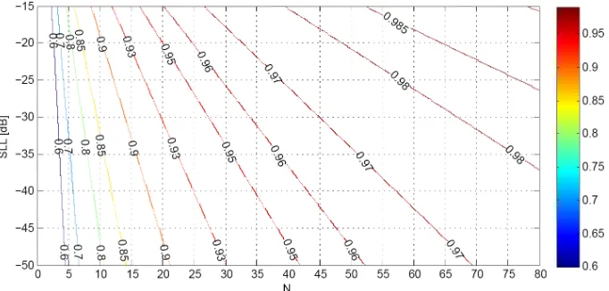
Let us now suppose thatu_s = 0, so the synthesized pattern is not going to be scanned. It is easy to plot the relationship between the SLL and the number of antenna elements for a variable beamwidth expressed in terms of u1,s (Fig. 1).

It is interesting to observe that the curves turn out to be well approximated by lines†, whose expression, found by polynomial regression is:

SLLdB(N, u, us = 0) =m0(u)N+q0(u)

m0(u) =−27.685u3+ 20.93u2−26.866u−0.008

q0(u) = 32.753u3 −22.716u2+ 27.055u+ 5.973

Figure 1. Relationship of the SLL and the number of antenna elements for a variable beamwidthu1,s.

Figure 2. Relationship of the SLL and the number of antenna elements for a variable inter-element distance d_E.

The maximum error with formula (7) is ±0.05 dB for the considered range (N from 2 to 80, SLLdB from −50 to−15).

Accordingly, it is possible to plot the relationship of the SLL and the number of antenna elements for a variable inter-element spacing d_E (Fig. 2). Even in this case the curves turn out to be well approximated by lines.

3. BENCHMARKING SYNTHESIS METHODS

As discussed in the Introduction, in this paper we propose to compare the performances achievable by some AUTs to the performances of the BEA. In order to have a correct benchmarking all the comparisons in the following sections have been realized according to these rules:

(i) Patterns are compared according to the same power pattern mask; in its definition strict inequalities are not used to avoid sampling ambiguities. The field is explicitly calculated in the angles defining the power pattern mask (f.i. u1).

Figure 3. Benchmarking of the results in [2, 9, 10].

Figure 4. Comparison with the pattern in [9].

3.1. First Example

As first example of the application of the proposed benchmarking procedure, let us now consider the sparse array obtained in [9] by means of a hybrid synthesis method. For this pattern u_s = 0,

u1 = 0.0399367, SLL=−20 dB and the number of employed elements isN = 25.

We can compare the SLL and number of elements of the aforementioned solution with the iso-beamwidth line relative to a BEA with u1 = 0.0399367 (see Fig. 3): the point relative to the solution with the hybrid method is on the left side of the curve.

This fact means that the AUT outperforms the reference BEA algorithm. The distance between the AUT point and the BEA curve at constant u1 gives an indication of the improvement of the AUT compared to the reference algorithm.

To get a better insight, the non-equispaced (N = 25) and the BEA (N = 26) patterns are plotted in Fig. 4; it is worth noting that the non-equispaced array presents a grating lobe just outside the range

3.2. A Second Example

As second example, we consider the result shown in [10], obtained using the matrix pencil method. For this patternu_s= 0,u1= 0.1372, SLL=−29.06 dB and the number of employed element is N = 12.

Even in this case we have compared the SLL and number of elements of the aforementioned solution with the iso-beamwidth line relative to a BEA withu1= 0.1372 (Fig. 3).

Differently from the previous case, the point relative to the solution in [10] is on the right side of the curve. This means that the AUT is outperformed by the reference BEA.

This behaviour is confirmed by the BEA pattern (shown in Fig. 5), that shows a better result in terms of SLL (for the BEASLLdB=−30.95 dB) using the same number of radiating elements; even in this case the non-equispaced array presents a grating lobe just outside the rangeu∈[−1,1], similarly to the BEA. It is also interesting to note that the excitation dynamic is of the same extent (about 12 dB) in the benchmarked pattern and the BEA pattern.

3.3. A Third Example

As last example, we consider the pattern reported in [2], obtained using an IGA-edsPSO. For this patternu_s= 0,u1= 0.1470, SLL=−26.67 dB and the number of employed element is N = 17.

Figure 5. Comparison with the pattern in [10].

If we compare the SLL and number of elements for the aforementioned solution with the iso-beamwidth line relative to a BEA withu1= 0.1470, we will find that the point relative to the solution in [2] is on the far right side of the curve, indicating that the AUT is outperformed by the reference BEA (see Fig. 3). It is interesting to observe that, in this case, the non equispaced array does not show a grating lobe for |u| > 1, but just an increase in the SLL. (Fig. 6). It is also worth noting that the elements’ excitation dynamic is about 14 dB in the AUT, while it is of about 12 dB in the BEA.

4. BEYOND PENCIL BEAMS

We must recall that the Dolph-Chebyshev excitation can only be used with a pencil beam, with constant symmetrical SLL. If a different power pattern mask is required, or we need to perform the synthesis including the effect of a specific element pattern, we could use convex programming [15, 17] for finding the optimal excitation for the array element.

Eventually, we could also modify the power pattern mask according to the method in [19] to achieve a constant SLL for the desired scanning range of the beam. The aforementioned “convex programming” approach could also be used when we have different radiating elements, variable orientations of the feeds or we need to take mutual coupling among elements into account using active element pattern methods [20].

It is also understood that, if the mutual coupling does not have a significant effect on the variation of the elements pattern, its presence does not change the results provided in Fig. 1 and Fig. 2, since the main effect of mutual coupling in that case is the modification of the vector of the imposed excitations on the radiating elements (letvbe) required to obtain the currents on the elements (i) used to calculate the radiated pattern‡.

To demonstrate the capability of the BEA to handle specifications “beyond pencil beams”, let us now consider some examples. It is not straightforward to obtain design curves for pattern specifications different from symmetrical pencil beams, but we can seek a BEA radiating a pattern that satisfies the same mask: the benchmarking will be done comparing the number of employed elements and the dynamic of the excitations.

4.1. Non-Symmetrical Wide-Scanning Pattern

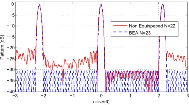
We will perform first the benchmarking of the 22 element array provided in [7]; this pencil beam array has a non-symmetrical power pattern defined in the rangeu∈[−22] in order to allow the beam scanning, without the appearance of grating lobes, in the whole visible range (so u_s = 1). In particular the side lobe level for the achieved pattern§ is below−21.356 dB foru≤ −0.1261 and it is below−30.328 dB for

u≥0.1238.

If we want to perform the benchmarking of this solution we first of all need to obtain the maximum allowed inter element distanced_E,s; by means of a simple manipulation of Eqs. (5) and (6) we can obtain it as:

d_E,s=λ(1 +u_s+u1,s)−1 (7)

In the considered case, by substituting u_s = 1 and u1,s = 0.1261 we obtain dE,s = 0.47034λ. It must be recalled that this inter-element distance is a maximum value, we are allowed to use smaller values (as far as we employ the necessary number of antennas).

The problem of finding the correct excitations for the BEA in this case can be solved by means of convex programming [17]. In particular by means of CVX [22] we can find that it is possible to satisfy the aforementioned specifications with d= 0.47034λ and N = 24. Because of the asymmetry of the excitations, it is possible to achieve a solution employing N = 23 elements by slightly reducing the inter-element distance to d= 0.465λ. A comparison of the pattern of [7] and the BEA pattern is provided in Fig. 7 while the achieved excitations are in Table 1. The result of the AUT outperforms the result of the BEA, since with the BEA we require one more radiating element to satisfy the same

‡ _{In that case we would have a linear relationship likev=CiwhereinCis a proper matrix depending on the geometry of the array,} the type and orientation of the radiating elements and the generators’ impedances [21].

Figure 7. Comparison for the asymmetric pencil beam pattern.

Table 1. Complex excitations w_k for the asymmetric pencil beam BEA.

w1= 0.02209−0.00431i w2= 0.01734−0.00290i w3= 0.02334−0.00360i w4= 0.02967−0.00403i

w5= 0.03645−0.00452i w6= 0.04312−0.00443i w7= 0.04947−0.00432i w8= 0.05522−0.00391i

w9= 0.06007−0.00308i w10= 0.06380−0.00214i w11= 0.06602−0.00128i w12= 0.06677 + 0.00000i

w13= 0.06601 + 0.00096i w14= 0.06362 + 0.00214i w15= 0.06010 + 0.00303i w16= 0.05527 + 0.00351i

w17= 0.04947 + 0.00405i w18= 0.04311 + 0.00433i w19= 0.03638 + 0.00409i w20= 0.02968 + 0.00400i

w21= 0.02322 + 0.00359i w22= 0.01747 + 0.00295i w23= 0.02230 + 0.00405i

constraints, but the excitation dynamic of the BEA is about 3 dB better than the excitation dynamic of the non-equispaced array (11.6 dB instead of 14.9 dB).

4.2. Flat Top Pattern

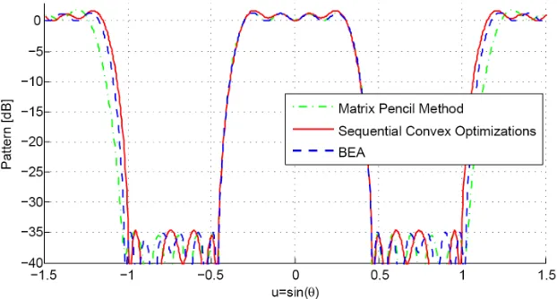
Let us consider now the flat-top shaped beam proposed in [16]. Such a 15 element array has been considered, with minor modifications, by other researchers [7, 12], who have tried to minimize the number of antennas needed with various synthesis techniques, and a minimum of 10 elements seems to be needed to achieve a pattern with similar specifications (0≤ |AF(u)|dB ≤1.27 for |u| ≤0.30595,

|AF(u)|dB ≤ −35 for|u| ≥0.457, and us= 0).

The element’s excitation will be chosen according to the technique described in [16]. If we calculate the maximum inter-element distance according to 8 we will find d_E,s = 0.68634λ; in this case it is possible to achieve a BEA satisfying the specifications with a number of elements as low asN = 11 with an inter-element distance d= 0.67λ. A comparison of the obtained pattern with the patterns achieved by other techniques is reported in Fig. 8, while the excitations for the BEA are provided in Table 2.

Finally, from a practical point of view, it is interesting to observe that the dynamic of the patterns in [7, 12] is about 25 dB, while in the BEA the excitation dynamic is about 13 dB, giving a more “stable” solution at the price of adding one radiating element.

Table 2. Complex excitations w_k for the “flat top”.

w1=−0.0825−0.0350i w2=−0.2296−0.0585i w3=−0.2766 + 0.0476i w4=−0.1486 + 0.2628i

w5=−0.0326 + 0.3474i w6=−0.1015 + 0.1503i w7=−0.2058−0.1298i w8=−0.1253−0.2060i

Figure 8. Comparison of the patterns for the flat-top.

Table 3. Complex excitations w_k for the “flat top” taking into account the element pattern.

w1= +0.07784 + 0.08928i w2= +0.09358 + 0.14079i w3= +0.00754 + 0.04300i w4= +0.04377−0.09893i

w5= +0.33653−0.08503i w6= +0.50501 + 0.00000i w7= +0.22553−0.01323i w8=−0.15707−0.02879i

w9=−0.17219 + 0.08272i w10= +0.02862 + 0.16264i w11= +0.06608 + 0.06603i w12=−0.03108−0.05867i

w13=−0.05309−0.06105i

4.3. Taking into Account the Element Pattern

As last example, we will discuss the case of of an array pattern in which we take into account the effect of the element factor in the synthesis. As an example we will consider the “case 4” analysed in [13], where a flat-top pattern, that takes into account a simple g(θ) = cos(θ) element pattern (with θ the angular direction with respect to the broadside), is synthesized. In such a paper the flat top pattern, whose mask is defined by−1≤ |F(u)|dB ≤0 for |u| ≤sin(20◦) and |F(u)|dB ≤ −30 for|u| ≥ sin(27◦), is realized with 19 elements.

According to Eq. (8) we can calculated_E,s= 0.68776λ; this value will not be a maximum one, since we are allowed to use slightly higher values than it, because of the effect of the element factor, that assumes very low values for directions far from the broadside, allowing the “grating lobes” of the array factor to partially enter in the visible range of the array, without affecting the final radiation pattern.

To perform the synthesis of the excitations, taking correctly into account the element factor, we have considered the synthesis of an array factor with a modified power pattern mask, according to the formula

˜

M_X(u) =M_X(u)/g2(u) (8)

whereM_X(u) is either the upper or lower power pattern mask, andg(u) is the element pattern. After some numerical trials, it turned out that the flat-top specifications can be met with an inter-element spacing d= 0.695λ, a slightly larger value than d_E,s, with only 13 radiating elements, instead of 19; the BEA in this case outperforms the AUT, with a reduction of the number of radiating elements of 6 (see Fig. 9 and Table 3).

4.4. Final Considerations

Summing up, when dealing with pattern specifications different from symmetrical pencil beams, we need first to find the inter-element distance d_E,s to avoid grating lobes then:

Figure 9. Pattern of the N = 13 element flat-top BEA, achieved considering the effect of the element factor. The pattern obtained in [13] is not reported because of the lack of the information on the excitations in the paper.

Table 4. Parameters of the power pattern mask for 4 “tough” problems; in the table we also provide the inter-element distance and the number of radiating elements of the corresponding BEA employing Dolph-Tchebyshev excitation.

# u1 SLLdB N dE[λ] # u1 SLLdB N dE[λ]

1 0.01982 −20 50 0.9805 2 0.1525 −20 8 0.867 3 0.111 −30 14 0.8999 4 0.0518 −25 24 0.9505

(iii) if the specifications are not met, try increasing the number of elements.

The aforementioned procedure usually allows, within few trials, to perform the benchmarking of the solution provided by the AUT. It must be underlined that when we deal with a synthesis method that takes into account the element pattern, we are also allowed increasing the inter-element distance with respect to d_E,s; anyway, the relative variation of the inter-element spacing with respect to d_E,s, in all the examples that we have considered (not reported for sake of brevity) has been at most of 3%.

Finally we have to emphasize that the computational power needed to perform all the examples in this paragraph is very small, the synthesis of the excitations typically required less than a three seconds on a office PC running Matlab, with a i5−2310 processor.

5. “TOUGH” PROBLEMS TO TEST YOUR ALGORITHMS

In this section we propose some “tough problems”, that can be useful in testing the capability of synthesis methods to achieve a significant solution. They are 4 particular pencil beams (their mask parameters are provided in Table 4), but can be also useful for testing algorithms designed for shaped beams: as we already discussed in the introduction, the fact that the AUT is capable to correctly solve a “simpler” problem can give a preliminary indication of the quality of the algorithm.

6. CONCLUSIONS

In this paper we introduce a method to benchmark the performances achievable by sparse linear array synthesis methods. The procedure is simple, and it is based on equispaced linear arrays with optimized spacing, that are taken as reference solution.

To demonstrate the procedure, we have applied it to the results obtained by some synthesis algorithms reported in literature. Unfortunately, in spite of the large number of papers on sparse synthesis, very few of them list the excitation coefficients of the synthesized array; among them we considered some papers reporting all the details required to reconstruct the patterns of the synthesized antennas. Unfortunately, for most of the array synthesis problems it is not possible to state which is the optimal solution, i.e., it is really hard to provide the maximum theoretical performance of an array under given electrical or geometrical constraints. The BEA would not provide the “best” results, but just a “sub-optimal” ones, to be used as reference. It has also to be stressed that if the solution provided by an AUT lies on the “left-side” of the BEA curve does not allow us to say how close we are with respect to the global optimum, but our approach is able to give a preliminary indication on the effectiveness of the synthesized layout.

To help interested researchers in benchmarking their algorithms, we have also proposed a list of “tough” problems that can provide a rough estimate of the quality of the AUT. We have also showed how it is possible to extend the use of BEA for benchmarking when dealing with specifications different from the symmetrical pencil beam ones; in particular we considered a non symmetrical pencil beam and two flat top patterns, in one of which we also take into account the effect of the element pattern.

It has to be noticed that in the shown comparisons, when the number of elements required for a BEA was higher with respect to other sparse arrays proposed in the open literature, such an increase was limited, and in many cases could be compensated by the simplification in the construction of an equispaced array. This does not mean that sparse non-equispaced arrays, and the synthesis techniques developed up to day, are not significant. We are sure that in some cases the authors of the AUTs have not chosen the proper examples to show the effectiveness of their results, even for the absence of a benchmarking tool like the one we are proposing in this contribution: in order to achieve an evaluation of the effective importance of the AUTs, it is important to compare the obtained results with the reference BEA and not to the λ/2 equispaced array.

We are currently working on the development of design curves for shaped beam cases (for instance, flat top beams), as well as on a specific extension of the benchmark procedure to planar and conformal arrays.

ACKNOWLEDGMENT

The authors would like to thank Dr. Benjamin Fuchs for his precious help in the realization of some of the numerical comparisons.

REFERENCES

1. Chen, K., Z. He, and C.-C. Han, “A modified real ga for the sparse linear array synthesis with multiple constraints,”IEEE Transactions on Antennas and Propagation, Vol. 54, No. 7, 2169–2173, 2006.

2. Zhang, S., S.-X. Gong, Y. Guan, P.-F. Zhang, and Q. Gong, “A novel IGA-edsPSO hybrid algorithm for the synthesis of sparse arrays,”Progress In Electromagnetics Research, Vol. 89, 121–134, 2009. 3. Barott, W. C. and P. G. Steffes, “Grating lobe reduction in aperiodic linear arrays of physically

large antennas,”Antennas and Wireless Propagation Letters, IEEE, Vol. 8, 406–408, 2009.

4. Goudos, S. K., K. Siakavara, T. Samaras, E. E. Vafiadis, and J. N. Sahalos, “Sparse linear array synthesis with multiple constraints using differential evolution with strategy adaptation,”Antennas and Wireless Propagation Letters, IEEE, Vol. 10, 670–673, 2011.

6. Oliveri, G. and A. Massa, “Bayesian compressive sampling for pattern synthesis with maximally sparse non-uniform linear arrays,”IEEE Transactions on Antennas and Propagation, Vol. 59, No. 2, 467–481, 2011.

7. Fuchs, B., “Synthesis of sparse arrays with focused or shaped beampattern via sequential convex optimizations,”IEEE Transactions on Antennas and Propagation, Vol. 60, No. 7, 3499–3503, 2012. 8. Pinchera, D. and M. D. Migliore, “Effective sparse array synthesis using a generalized alternate projection algorithm,”2014 IEEE Conference on Antenna Measurements&Applications (CAMA), 1–2, 2014.

9. Isernia, T., F. Ares, O. M. Bucci, M. D’Urso, J. F. Gomez, and J. Rodriguez, “A hybrid approach for the optimal synthesis of pencil beams through array antennas,”IEEE Antennas and Propagation Society International Symposium, Vol. 3, 2301–2304, 2004.

10. Liu, Y., Z. Nie, and Q. H. Liu, “Reducing the number of elements in a linear antenna array by the matrix pencil method,” IEEE Transactions on Antennas and Propagation, Vol. 56, No. 9, 2955–2962, 2008.

11. Manica, L., P. Rocca, and A. Massa, “Design of subarrayed linear and planar array antennas with sll control based on an excitation matching approach,” IEEE Transactions on Antennas and Propagation, Vol. 57, No. 6, 1684–1691, 2009.

12. Liu, Y., Q. H. Liu, and Z. Nie, “Reducing the number of elements in the synthesis of shapedbeam patterns by the forward-backward matrix pencil method,” IEEE Transactions on Antennas and Propagation, Vol. 58, No. 2, 604–608, 2010.

13. Nai, S. E., W. Ser, Z. L. Yu, and H. Chen, “Beampattern synthesis for linear and planar arrays with antenna selection by convex optimization,”IEEE Transactions on Antennas and Propagation, Vol. 58, No. 12, 3923–3930, 2010.

14. Dolph, C., “A current distribution for broadside arrays which optimizes the relationship between beam width and side-lobe level,” Proceedings of the IRE, Vol. 34, No. 6, 335–348, 1946.

15. Lebret, H. and S. Boyd, “Antenna array pattern synthesis via convex optimization,” IEEE Transactions on Signal Processing, Vol. 45, No. 3, 526–532, 1997.

16. Isernia, T., O. Bucci, and N. Fiorentino, “Shaped beam antenna synthesis problems: Feasibility criteria and new strategies,” Journal of Electromagnetic Waves and Applications, Vol. 12, No. 1, 103–138, 1998.

17. Isernia, T., P. D. Iorio, and F. Soldovieri, “An effective approach for the optimal focusing of array fields subject to arbitrary upper bounds,”IEEE Transactions on Antennas and Propagation, Vol. 48, No. 12, 1837–1847, Dec. 2000.

18. Fuchs, J.-J. and B. Fuchs, “Synthesis of optimal narrow beam low sidelobe linear array with constrained length,” Progress In Electromagnetics Research B, Vol. 25, 315–330, 2010.

19. Bucci, O. M., T. Isernia, S. Perna, and D. Pinchera, “Isophoric sparse arrays ensuring global coverage in satellite communications,” IEEE Transactions on Antennas and Propagation, Vol. 62, No. 4, 1607–1618, 2014.

20. Kelley, D. F. and W. L. Stutzman, “Array antenna pattern modeling methods that include mutual coupling effects,” IEEE Transactions on Antennas and Propagation, Vol. 41, No. 12, 1625–1632, 1993.

21. Hui, H. T., “Decoupling methods for the mutual coupling effect in antenna arrays: A review,” Recent Patents on Engineering, Vol. 1, No. 2, 187–193, 2007.

22. “Cvx: Matlab software for disciplined convex programming,” [Online]. Available: