Load Frequency Control of A Multi-Area Power System

(1)

ISSN (Print) : 2320 – 3765 ISSN (Online): 2278 – 8875

I

nternational

J

ournal of

A

dvanced

R

esearch in

E

lectrical,

E

lectronics and

I

nstrumentation

E

ngineering

(An ISO 3297: 2007 Certified Organization)

Vol. 5, Issue 5, May 2016

Load Frequency Control of A Multi-Area

Power System

D. Saraswathi, K. Lokanadham,

PG Student, Dept of EEE, Sri Venkateswara College of Engineering & Technology (Autonomous), Chittoor, AP, India Associate Professor, Dept of EEE, Sri Venkateswara College of Engineering & Technology (Autonomous), Chittoor,

AP, India

ABSTRACT: Load Frequency Control (LFC) of a multi-area power systems is developed based on the Bacteria Foraging Optimization Algorithm (BFOA). Variations in load bring about drifts in frequency and voltage which in turn leads to generation loss owing to the line tripping and also blackouts. These drifts might be reduced to the smallest possible value by automatic generation control (AGC) which constitutes of two sections viz load frequency control (LFC) along with automatic voltage regulation (AVR). LFCs for each area are designed based on availability of frequency deviation of each area and tie-line power deviation between areas. Several important parameters of ALFC like integral controller gains (KIi), parameters for governor speed regulation (Ri) as well as parameters for frequency bias (Bi) are being optimized by using an optimization technique that is Bacteria Foraging Optimization Algorithm (BFOA) because using DIAFLC simulation has some demerits which has insisted on using BFOA for obtaining the desired values of the different parameters. In the presence of parameter uncertainties and unknown saturation and dead band of GRC and GDB which grants not only the best dynamic response for the system but also permits us to show the zero steady state frequency and tie line power deviation. Simulation results for a real three-area power system prove the effectiveness of the proposed LFC and show its superiority over a classical PID controller,DIAFLC Controller and a type-2 fuzzy controller.

KEYWORDS: BFOA,GDB, GRC, load frequency control (LFC),multi-area. I .INTRODUCTION

Bacterial Foraging Optimization Algorithmic Program (BFOA) could be a Global Optimization Algorithmic Program for Distributed Control, Management and Optimization. Each bacterium looks around for nutrients in order to make the most of energy acquired per unit time. Individual bacterium simultaneously keeps up a correspondence with others by delivering signals. An individual bacterium will take foraging judgment after taking into consideration two prior factors. The process when a bacterium is all set for finding the nutrients with small steps is named as chemo taxis and principle concept of BFOA is chemo tactic locomotion mimicking within the region of problem search for the virtual bacterium.

Bacteria discover the direction to food in the surroundings on the basis of the gradients of chemicals. Similarly, bacterium secretes attracting along with repellant chemicals into the surroundings and is able to discover one another in the similar way. Locomotion mechanisms with the help of flagella, bacterium is used to make it able to move about in their surroundings, sometimes going around wildly (tumbling and spinning), and rest of the times moving in a determined path (swimming). The bacterial cells are usually treated resembling mediators in particular surroundings, by means of their food perception and various other cells as a motivating factor to move about, and random tumbling as well as swimming movement on the way to relocate. On the basis of the cell-cell interactions, cells might swarm a source of food, and/or mightdirectly repel or else ignore one another.

(2)

I

nternational

J

ournal of

A

dvanced

R

esearch in

E

lectrical,

E

lectronics and

I

nstrumentation

E

ngineering

Vol. 5, Issue 5, May 2016

number, the total swim steps for a given cell, a random direction vector with identical range of dimensions because the problem region, and also the cells probability of being subjected to elimination plus dispersal.

II DYNAMIC MODEL OF A MULTI-AREA POWER SYSTEMS

Consider a power system consisting of LFC areas; each area has a number of generators. All generators in one area are simplified as an equivalent generator unit. Moreover, each area is assumed to have a number of gas turbines of

simple cycle and combined cycle types and a number of steam turbines of reheat type. Without loss of generality, it is assumed that the controller to be proposed is installed to the gas turbines. While the steam turbines have no control

on the reference set-point. The nonlinearities of the GRC and the GDB are incorporated in the model as nonlinear functions

_

1 1 1

(

,

),

(

)

i

P

_{t i}

P

_{g i}

and

_i

P

_{g i}





respectively. The block diagram of the LFC area in a multi-area system is shown in Fig 1

The dynamic model of each area can be written as:

. _ __ __ __ __ __ __ __ __ __ __ __ 1 2 1 N

ii i i i

i i i i ij j i i di

j

x A x B u E r A x g g F P



   

_

   (1)

__ __

i

i i

y C x

(2) where the control area matrices are given by

__

0 0 0 0 0 0 0

2 0 0 0 0 0 0

ij ij A T                        __ 1

1 [0 0

0 0 0 0]

T i g i

B

T



__

₁

[

0 0

0 0 0 0]

T

i i

F

M



__

[0

0 0 0

0 1 0]

T i

E



__

[1

0 0 0

0 0 0]

i

C



__ __ __

1

0

0 0 0 0 0

T i i i

g

x

M













_

_

_

_









and __ i

x

_and

__

,

ii

A

shown at the bottom of the following

__ __ __

1

2

(1/

)[0

(

) 0 0 0 0 0]

T i

i t i i

g



T



x

and

__

i

r

is the change in reference set-point of the steam turbine (assumed zero), is the load change,

T

ij



T

ji

,

and

2

(

K

_ri

/

T

_{g i}

)

(1/

T

_ri

))

(3)

I

nternational

J

ournal of

A

dvanced

R

esearch in

E

lectrical,

E

lectronics and

I

nstrumentation

E

ngineering

Vol. 5, Issue 5, May 2016

functions

__

2 3

(

,

)

i

x x



and



_i

( )

x

₃ are assumed unknown. To facilitate the design of a local model (1) is transformed to the controller canonical from as

Fig.1: Dynamic model of the ith area in a multi-area power system

.

1 2

1, 1

( )

N

i _ii _i _i _i _ij _j _i _i _i _i _di

j j

x

A x

B u

A x

g

x

g

x

F P

 





_





(3)

i i i

y Cx



(4) where

__ __ __ __ __ __ __ __

1 1 1 1 1 1

1 1 2 2

,

ii i i ij i

ii i i i i i i ij i j i i i i i i i i

A



S



A S B



S



B F



S



F A



S



A S C



C S g



S



g



S



g

and

i

S

is the similarity transformation matrix. Equation (3) can be written in the following form:

.

1

( )

i _{ii i} _i _i _i _i _i _i

x



A x



B u



D X



G x



F

(5)

where

D

_iT

(

X

)



[

D

₁_i

(

X

)...

D

₇_i

(

X

)]

accounts for the interconnections between the ith area and other areas

1

( )

[

11

( )...

71

( )]

2

( )

[

12

( )...

72

( )]

T T

i i i i i i i i i i i i

G

x



G

x

G

x G

x



G

x

G

x

represent the GRC and GDB non linearity’s.

1 7

( )

[

]

T

i i i i

F

x



F



F

represents the load disturbance terms, and the vector

X



[

x x

_{1 2}

...

x

_N

]

is the composite state vector.

The ith isolated and undisturbed LFC area of the model (5) without consideration of GDB and GRC nonlinearities is given by

.

i _ii _i _{i i}

x



A x



B u

(6)

where the transformed matrices

A B

ii

,

i and

C

i have the forms

0 1 2 3 4 5 6

0 1 0 0 0 0 0

0 0 1 0 0 0 0

0 0 0 1 0 0 0

0 1 0 0 1 0 0

0 1 0 0 0 1 0

0 1 0 0 0 0 1

ii

i i i i i i i

A

a a a a a a a

                   _ _ _ _ _ _ _   

[0 0 0 0 0 0 1]

T i

B



0 1 2 3 4

[

0 0]

i i i i i i

(4)

I

nternational

J

ournal of

A

dvanced

R

esearch in

E

lectrical,

E

lectronics and

I

nstrumentation

E

ngineering

Vol. 5, Issue 5, May 2016

The entries of the last row of

A

_iidenoted by

a

i

 

[

a

ji

],

j



0,...6,

and

i



1,...

N

are negative and dependent on system parameters.

The transfer function of (6) is given by

4 3 2

4 3 2 1 0

7 6 5 4 3 2

6 5 4 3 2 1 0

( )

i i i i i

i

i i i i i i i

c s

c s c

H s

s

a s

a s a







( )

i i

N s

D s



(7) xi=[∆fi ∆Pg1i ∆Pt2i ∆Pri ∆Ptiei]

1 1 1 1 __ 2 2 2 2 2 1, 1

1 1 1

0 0 0

1 1

0 0 0 0 0

1 1

0 0 0 0 0

1 1

0 0 0 0 0

1

0 0 0 0

1 1

0 0 0 0 0

2 0 0 0 0 0 0

i

i i i i

t i t i

i g i g i

ii

t i t i

i g i ri

i g i g i

N j j D

M M M M

T T

R T T

A

T T k

R T T

T     _ _                                                  

Upon repetitive differentiation of (4) and using (6) until the input appears, one can obtain

..

3 2

i ii i i ii i i i

y



C A x



C A B u

(8)

where

C A x

_i _ii3 _i



c a x

₄_i _i _i



[0 0 0

co c

_i ₁_i

c

₂_i

c

₃_i

]

T

x

_i and

C A B u

i ii2 i i



c u c

4i i

,

4_i



0.

Equation (8) indicates

that the relative degree of each subsystem is 3. This means that its zero dynamics is of order 4. In fact the poles of reciprocal of the polynomial

N s

_i

( )

represents the zero dynamics which is stable provided that

c

_ki



0,

k



0,...4.

If the parameters of subsystem (4) and (6) are precisely known, the ideal local control can be written as

..

* 3

4

1

T

i ri i i i ii i

i

u

y

K e

C A x

c







_





_





₍₉₎

where

y

_riis a reference signal, assumed to have bounded derivatives (up to 3). The control law (9) will force the error vector

. ..

[

i i

]

T

i i

e



e e

e

to converge to zero where

e

_i



y

_ri



y

_i provided

K

_i



[

K K K

_oi ₁_i ₂_i

]

T is chosen such that all of the roots of the characteristic equation

s

3



K s

₂_i 2



K s

₁_i



K

₀_i



0

are in the open left half of the S-plane.

III. BFO ALGORITHM

A: Parameters Initialization

(5)

I

nternational

J

ournal of

A

dvanced

R

esearch in

E

lectrical,

E

lectronics and

I

nstrumentation

E

ngineering

Vol. 5, Issue 5, May 2016

 P = total quantity of parameters to be optimized. Here either KIi or (KIi andRi) or (KIi , Ri andBi) are

optimized.



S

_s = length of swimming subsequent to which the tumbling takes place in a Chemotactic loop.



S

_c = iterations number in a chemo tactic loop.



S

_re = utmost number of steps of reproduction.



S

_ed = utmost number of elimination and dispersal action forced on the bacteria.



P

_ed = probability for the continuation of elimination as well as dispersal process.

 Each bacterium P has a location that is stated by the arbitrary quantities within the range of [-1, 1].

 Value of C(a) is considered to be fixed for simplification.

 Values of

d

attract

,

w

attract

,

h

repelent

and w

repelent_. B: Optimization

Step-1: Elimination-dispersal loop: d=d+1

Step-2: Reproduction loop: c=c+1

Step-3: Chemo taxis loop: b=b+1

i. For a =1, 2,…S take a chemo tactic step for bacterium a and calculate fitness function, J(a, b, c, d). Let,

( , , , )

(

a

( , , ), ( , , ))

sw cc

J

a b c d



J a b c d



J



b c d P b c d

(i.e. insert on the cell-to cell attractant–repellant effect/profile for simulating the behavior of swarming)

Where,

1

2 2

1 1 1 1

( , ( , , )) ( , ( , , ))

[ exp( ( ) ] [ exp( ( ) ]

S

a a

cc cc

a

p p

S S

m a m a

attract attract m repelent repelent m

a m a m

J P b c d J b c d

d h

  

     



   



       



( , , , )

last sw

J



J

a b c d

to preserve this quantity because we might get a improved cost through a run.

End for this loop

ii. For a = 1, 2,..S tumble/swim decision is taken.

 Tumble: The random vector Δ(a) is generated on [-1, 1]. Let

( )

(

1, , )

( , , )

( )

( ) ( )

a a

T

a

b

c d

b c d

C a

a













(6)

I

nternational

J

ournal of

A

dvanced

R

esearch in

E

lectrical,

E

lectronics and

I

nstrumentation

E

ngineering

Vol. 5, Issue 5, May 2016

( ,

1, , )

( ,

1, , )

(

a

(

1, , ), (

1, , ))

sw cc

J

a b



c d



J a b



c d



J



b



c d P b



c d

 Swim:

Let mswim=0 (counter for swim length).

While mswim< Ss (if haven’t brought down excessively long). Let mswim=mswim+1.

If Jsw (a, b + 1, c , d) =Jlast ( if doing better), let Jlast = Jsw (a, b + 1, c , d) and Let

( )

(

1, , )

( , , )

( )

( ) ( )

a a

T

a

b

c d

b c d

C a

a













And use this



a

(

b



1, , )

c d

to find the new

J a b

( ,



1, , )

c d

Else, let

m

_swin



S

_s This Ends the while statement

iii. Go to the just succeeding bacterium (a+1) suppose a ≠ S (i.e., go to [ii] to continue with the successive bacterium).

Step-4: If b < Sc , proceed on to step 3 and carry on with the chemo taxis process since the lifetime of the bacteria isn’t ended.

Step-5: Reproduction

i. For the known c and d, and for every a = 1,2,…, S , let

1

( , , , )

c

S a health

b

J

J a b c d





_

be the fitness of the bacterium a (a quantity of the number of nutrients it acquired during its lifespan moreover how efficient it was at overcoming toxic substances).

Arrange bacteria and also chemo tactic parameters C (a) in sort of ascending cost

health

J

(high cost gives low health).

ii. The

S

_r



S

/ 2

bacterium with the maximum J health values die and the rest of the Sr bacteria possessing the best values divide (this method is performed by the group of bacteria that are being placed at the similar location where the parent was present).

Step-6: If

c



S

_re, proceed on to step 3 because we haven’t reached the specified quantity of reproduction steps and therefore we begin the succeeding generation of the chemo tactic loop.

Step-7: Elimination-dispersal: For a = 1,2..., S possessing probability

P

_edevery bacterium is eliminated and dispersed so as to keep the quantity of bacteria present in the population to a constant value. During this process if a bacterium is removed then simply scatter a new one to any arbitrary position on the optimization domain.

When d =

S

_edthen move on to step 2 else end it.

Step-8: Obtain the optimized values of the parameters.

(7)

I

nternational

J

ournal of

A

dvanced

R

esearch in

E

lectrical,

E

lectronics and

I

nstrumentation

E

ngineering

Vol. 5, Issue 5, May 2016

Area -2

T

₁₂

T

₁₃ Area -3

Area -1 Fig .2 Three area system

(8)

I

nternational

J

ournal of

A

dvanced

R

esearch in

E

lectrical,

E

lectronics and

I

nstrumentation

E

ngineering

Vol. 5, Issue 5, May 2016

Table I: System parameters Table II: Controller Parameters Parameter Area-1 Area-2 Area-3

D

0.24 0.11 0.046

r

K

0.3 0.3

M

167 89.5 23.25

R

0.04 0.04 0.04

1

t

T

0.4 0.4 0.1

1

g

T

0.1 0.1 0.4

2

t

T

1.0 1.0

2

g

T

0.1 0.1

ri

T

1.0 1.0

12 21

T



T

8.4 8.4

13 31

T



T

2.3 2.3

Table III: If–Then rules for the type-2 fuzzy controller

ACE N Z P

N P N N

Z N P P

P N N N

IV .SIMULATION RESULTS

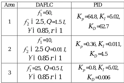
A real three-area interconnected power system existing in the gulf region is considered as a simulation example to investigate the effectiveness of the proposed BFOAlogrithm.The three area power system is shown in fig.3.The system parameters are given table 1. It is assumed that no fuzzy control rules are available for the proposed BFOA.Comparisons between simulation results of the proposed BFOA and those of a PID classical controller, designed using Ziegler-Nichols method, and a type-2 fuzzy decentralized LFC(Type-2 Fuzzy) ,DIAFLC are carried out in the presence of GRC and GDB. The parameters of the DIAFLC and the PID controller are tabulated in Table II and the “If-then” rules for the Type-2 fuzzy controller are given in Table III.

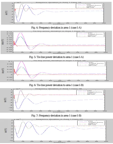
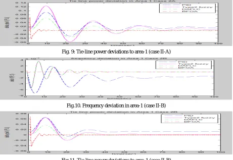
Two different simulation cases are considered. In case I, the nominal parameters of the system are used, and two simulation tests are carried out, namely, a load disturbance of 300 MW (0.3 p,u,) is assumed to take place in area-1 (case A) and load disturbances of 0.3, 0.1, and 0.01 p.u. are assumed to occur in areas 1, 2, and 3, respectively (case I-B). The off-nominal parameters are considered in case II. In this case, two simulation sets of results are obtained. In the first set a mismatch of 50% in both the inertia constant and load damping coefficient is assumed(case II-A). The second set where the tie-line synchronizing power coefficient has amismatch of 50% is considered (case II-B). Simulation results of the frequency and the tie-line power deviations of area 1 for case I-A are shown in Figs. 4 and 5. Frequency and tie-line power deviations of area 1 for case I-B are shown in Figs. 6 and 7. Simulation results for cases A and II-B are given in Figs. 8–11, respectively.

Area DAFLC PID

1



=50,

2

2.5 



,

Q

=1.5 I,

0.85 



,

r



1

p

K

=64.8,

K

I=5.02, D

K

=62.7

2

1



=10,

2

2.5 



Q

=0.01 I,

0.85 



r



1

p

K

=0.36,

K

_I=0.011,

D

K

=4.5

3



1=25,

Q

=0.5 I,

0.85 



r



1

p

K

=0.8,

K

_I=5.02,

D

(9)

I

nternational

J

ournal of

A

dvanced

R

esearch in

E

lectrical,

E

lectronics and

I

nstrumentation

E

ngineering

Vol. 5, Issue 5, May 2016

Fig. 4: Frequency deviation in area-1 (case I-A)

Fig. 5: Tie-line power deviation to area-1 (case I-A)

Fig. 6: Tie-line power deviation to area-1 (case I-B)

Fig .7: Frequency deviation in area-1 (case I-B)

(10)

I

nternational

J

ournal of

A

dvanced

R

esearch in

E

lectrical,

E

lectronics and

I

nstrumentation

E

ngineering

Vol. 5, Issue 5, May 2016

Fig. 9: Tie-line power deviations to area-1 (case II-A)

Fig.10. Frequency deviation in area-1 (case II-B)

Fig.11. Tie-line power deviations to area-1 (case II-B)

A summary of simulation performance in terms of the steady-state and maximum overshoot( of frequency deviation for area 1 and the steady-state and maximum overshoot of tie-line power deviation for area 1 of the three controller is shown in below tabular column.

Table 4: Performance comparison in terms of the steady state frequency deviation for area 1

Case BFOA DAFLC Type-2 Fuzzy PID Case

1A 0 0 0 9

Case 1B 0.000256 0.004497 0.044452 9.306719 Case

(11)

I

nternational

J

ournal of

A

dvanced

R

esearch in

E

lectrical,

E

lectronics and

I

nstrumentation

E

ngineering

Vol. 5, Issue 5, May 2016

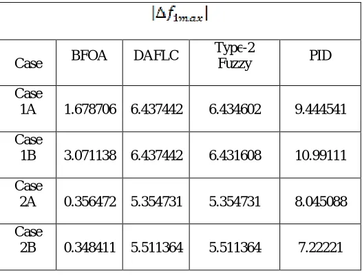
Table 5: Performance comparison in terms of the maximum overshoot frequency deviation for area 1

Table 6: Performance comparison in terms of the steady state tie line power deviation for area 1 Case BFOA DAFLC

Type-2

Fuzzy PID

Case

1A 1.678706 6.437442 6.434602 9.444541 Case

1B 3.071138 6.437442 6.431608 10.99111 Case

2A 0.356472 5.354731 5.354731 8.045088 Case

2B 0.348411 5.511364 5.511364 7.22221

Case

BFOA DAFLC

Type-2

Fuzzy PID

Case

1A 0 0 0 10

Case

1B 0.023727 0.302367 5.044261 7.808516 Case

2A 0.038948 0.638686 0.086975 15.79836 Case

(12)

I

nternational

J

ournal of

A

dvanced

R

esearch in

E

lectrical,

E

lectronics and

I

nstrumentation

E

ngineering

Vol. 5, Issue 5, May 2016

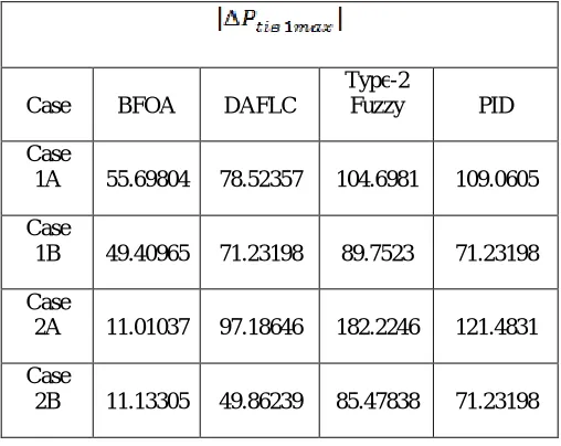
Table 7: Performance comparison in terms of the maximum overshoot tie line power deviation for area 1

Case BFOA DAFLC

Type-2

Fuzzy PID Case

1A 55.69804 78.52357 104.6981 109.0605 Case

1B 49.40965 71.23198 89.7523 71.23198 Case

2A 11.01037 97.18646 182.2246 121.4831 Case

2B 11.13305 49.86239 85.47838 71.23198

It is clear that the BFOA achieves the LFC objectives even in the presence of parameter uncertainties and unknown saturation and dead band of GRC and GDB. It is worth-noting to mention that the advantage of the BFOA is that it does not need any set of “if-then” rules in contrast to the type-2 fuzzy controller and it can cope with parameter variation and the unknown nonlinearities. However, from the comparison table, and of the BFOA is higher than those of the PID, DIAFLCand Type-2 Fuzzy controller

V.CONCLUSION

Load frequency control of multi-area power system having unknown parameters. The proposed algorithm is developed using BFOA technique. Bacteria Foraging Optimization Algorithmic program to change the values of the various parameters present in the power system under investigation so it can cope up with the presence of parameter uncertainties and unknown saturation and dead band of GRC and GDB.. As a result of which the changes the frequency and also the tie line power is reduced and also the stability of the system is maintained. BF technique serves to be quite useful for obtaining the optimized values of the various parameters as compared to DIAFLC technique which is extremely tedious and time taking method. A realistic three-area power system is used as a validation example.Simulation results show that the developed BFOA is able to achieve the LFC objectives in terms of zero steady-state frequency and tie-line deviations. Superiority of the developed BFOA over a DIAFLC,Type-2 fuzzy and a classical PID controller is illustrated.

REFERENCES

[1]I J Nagrath and D. P Kothari Modern power system analysis- TMH 1993.

[2]R. Arivoli and I. A. Chidambaram, “CPSO based LFC for a two-area power system with GDB and GRC nonlinearities interconnected through TCPS in series with the tie-line,” Int. J. Comput. Applications,vol. 38, no. 7, pp. 1–10, Jan. 2012.

[3]S. Velusami and I. A. Chidambaram, “Decentralized biased dual mode controllers for load frequency control of interconnected power systems considering GDB and GRC non linearities,” Energy Convers. Manag., vol. 48, pp. 1691–1702, 2007.

[4]Wen Tan, “Unified tuning of PID load frequency controller for power systems via IMC”, IEEE Transactions on Power Systems, vol.25, no.1, pp.341-350, 2010.[5]U.K.Rout, R.K.Sahu, S.Panda, “Design and analysis of differential evolution algorithm based automatic generation control for interconnected power system”, Ain Shams Engineering Journal, vol. 4, No. 3, pp. 409, 2013.

[5]J.Nanda, S.Mishra and L.C.Saikia, “Maiden Application of Bacterial Foraging Based Optimization Technique in Multiarea Automatic Generation Control”, IEEE Transactions on Power Systems, vol. 22, No.2, pp.602-609, 2009.