Volume 2006, Article ID 26318, Pages1–19 DOI 10.1155/ASP/2006/26318
Denoising by Sparse Approximation: Error Bounds
Based on Rate-Distortion Theory
Alyson K. Fletcher,1Sundeep Rangan,2Vivek K Goyal,3and Kannan Ramchandran4
1Department of Electrical Engineering and Computer Sciences, University of California, Berkeley, CA 94720-1770, USA 2Flarion Technologies Inc., Bedminster, NJ 07921, USA
3Department of Electrical Engineering and Computer Science and Research Laboratory of Electronics,
Massachusetts Institute of Technology, Cambridge, MA 02139-4307, USA
4Department of Electrical Engineering and Computer Sciences, College of Engineering, University of California, Berkeley,
CA 94720-1770, USA
Received 9 September 2004; Revised 6 June 2005; Accepted 30 June 2005
If a signalxis known to have a sparse representation with respect to a frame, it can be estimated from a noise-corrupted observation yby finding the best sparse approximation toy. Removing noise in this manner depends on the frame efficiently representing the signal while itinefficientlyrepresents the noise. The mean-squared error (MSE) of this denoising scheme and the probability that the estimate has the same sparsity pattern as the original signal are analyzed. First an MSE bound that depends on a new bound on approximating a Gaussian signal as a linear combination of elements of an overcomplete dictionary is given. Further analyses are for dictionaries generated randomly according to a spherically-symmetric distribution and signals expressible with single dictionary elements. Easily-computed approximations for the probability of selecting the correct dictionary element and the MSE are given. Asymptotic expressions reveal a critical input signal-to-noise ratio for signal recovery.
Copyright © 2006 Alyson K. Fletcher et al. This is an open access article distributed under the Creative Commons Attribution License, which permits unrestricted use, distribution, and reproduction in any medium, provided the original work is properly cited.
1. INTRODUCTION
Estimating a signal from a noise-corrupted observation of the signal is a recurring task in science and engineering. This paper explores the limits of estimation performance in the case where the onlya prioristructure on the signalx ∈RN
is that it has known sparsityKwith respect to a given set of vectorsΦ = {ϕi}Mi=1 ⊂ RN. The setΦis called adictionary and is generally aframe[1,2]. The sparsity ofKwith respect toΦmeans that the signalxlies in the set
ΦK=
v∈RN |v= M
i=1
αiϕiwith at mostKnonzeroαi’s
.
(1) In many areas of computation, exploiting sparsity is mo-tivated by reduction in complexity [3]; ifK N, then cer-tain computations may be more efficiently made onαthan onx. In compression, representing a signal exactly or approx-imately by a member ofΦK is a common first step in effi
-ciently representing the signal, though much more is known whenΦ is a basis or union of wavelet bases than is known in the general case [4]. Of more direct interest here is that
sparsity models are becoming prevalent in estimation prob-lems; see, for example, [5,6].
The parameters of dimensionN, dictionary sizeM, and sparsityKdetermine the importance of the sparsity model. Representative illustrations ofΦKare given inFigure 1. With
dimensionN=2, sparsity ofK=1 with respect to a dictio-nary of sizeM=3 indicates thatxlies on one of three lines, as shown inFigure 1a. This is a restrictive model, even if there is some approximation error in (1). WhenMis increased, the model stops seeming restrictive, even though the set of possi-ble values forxhas measure zero inR2. The reason is that un-less the dictionary has gaps, all ofR2is nearly covered. This paper presents progress in explaining the value of a sparsity model for signal denoising as a function of (N,M,K).
1.1. Denoising by sparse approximation with a frame
Consider the problem of estimating a signalx ∈ RN from
the noisy observationy=x+d, whered∈RN has the i.i.d.
GaussianN(0,σ2I
N) distribution. Suppose we know thatx
lies in givenK-dimensional subspace ofRN. Then projecting
(a) (b)
Figure1: Two sparsity models in dimensionN = 2. (a) Having sparsityK =1 with respect to a dictionary withM=3 elements restricts the possible signals greatly. (b) With the dictionary size in-creased toM=100, the possible signals still occupy a set of measure zero, but a much larger fraction of signals is approximately sparse.
without affecting the signal component. Denoting the pro-jection operator byP, we would have
x=P y=P(x+d)=Px+Pd=x+Pd, (2)
andPdhas onlyK/N fraction of the power ofd.
In this paper, we consider the more general signal model x ∈ ΦK. The setΦK defined in (1) is the union of at most
J =M K
subspaces of dimensionK. We henceforth assume thatM > K (thus J > 1); if not, the model reduces to the classical case of knowing a single subspace that containsx. The distribution ofx, if available, could also be exploited to remove noise. However, in this paper the denoising operation is based only on the geometry of the signal modelΦKand the
distribution ofd.
With the addition of the noised, the observed vectory will (almost surely) not be represented sparsely, that is, not be inΦK. Intuitively, a good estimate forxis the point fromΦK
that is closest to yin Euclidean distance. Formally, because the probability density function ofdis a strictly decreasing function ofd2, this is the maximum-likelihood estimate ofxgiveny. The estimate is obtained by applying an optimal sparse approximation procedure toy. We will write
xSA=arg min
x∈ΦK
y−x2 (3)
for this estimate and call it the optimalK-term approxima-tion ofy. Henceforth, we omit the subscript 2 indicating the Euclidean norm.
The main results of this paper are bounds on the per-component mean-squared estimation error (1/N)E[x −
xSA2] for denoising via sparse approximation.1 These bounds depend on (N,M,K) but avoid further dependence on the dictionaryΦ(such as the coherence ofΦ); some re-sults hold for allΦand others are for randomly generatedΦ.
1The expectation is always over the noisedand is over the dictionaryΦ and signalxin some cases. However, the estimator does not use the dis-tribution ofx.
To the best of our knowledge, the results differ from any in the literature in several ways.
(a) We study mean-squared estimation error for additive Gaussian noise, which is a standard approach to per-formance analysis in signal processing. In contrast, analyses such as [7] impose a deterministic bound on the norm of the noise.
(b) We concentrate on having dependence solely on dic-tionary size rather than more fine-grained properties of the dictionary. In particular, most signal recov-ery results in the literature are based on noise being bounded above by a function of thecoherenceof the dictionary [8–14].
(c) Some of our results are for spherically symmetric ran-dom dictionaries. The series of papers [15–17] is su-perficially related because of randomness, but in these papers, the signals of interest are sparse with respect to a single known, orthogonal basis and the observations are random inner products. The natural questions in-clude a consideration of the number of measurements needed to robustly recover the signal.
(d) We use source-coding thought experiments in bound-ing estimation performance. This technique may be useful in answering other related questions, especially in sparse approximation source coding.
Our preliminary results were first presented in [18], with fur-ther details in [19,20]. Probability of error results in a rather different framework for basis pursuit appear in a manuscript submitted while this paper was under review [21].
1.2. Connections to approximation
A signal with an exactK-term representation might arise be-cause it was generated synthetically, for example, by a com-pression system. A more likely situation in practice is that there is an underlying true signalxthat has a goodK-term approximationrather than an exactK-termrepresentation. At very least, this is the goal in designing the dictionaryΦfor a signal class of interest. It is then still reasonable to compute (3) to estimatexfromy, but there are tradeoffs in the selec-tions ofKandM.
Let fM,K denote the squared Euclidean approximation
error of the optimal K-term approximation using an M-element dictionary. It is obvious that fM,Kdecreases with
in-creasingK, and with suitably designed dictionaries, it also decreases with increasing M. One concern of approxima-tion theory is to study the decay of fM,Kprecisely. (For this,
we should consider Nvery large or infinite.) For piecewise smooth signals, for example, wavelet frames give exponential decay withK[4,22,23].
of subspaces, and thus increases the chance that the selected subspace is not the best one for approximating x. Loosely, whenMis very large and the dictionary elements are not too unevenly spread, there is some subspace very close toy, and thusxSA≈y. This was illustrated inFigure 1.
Fortunately, there are many classes of signals for which Mneed not grow too quickly as a function ofNto get good sparse approximations. Examples of dictionaries with good computational properties that efficiently represent audio sig-nals were given by Goodwin [24]. For iterative design proce-dures, see papers by Engan et al.[25] and Tropp et al.[26].
One initial motivation for this work was to give guidance for the selection ofM. This requires the combination of ap-proximation results (e.g., bounds on fM,K) with results such
as ours. The results presented here do not address approxi-mation quality.
1.3. Related work
Computing optimal K-term approximations is generally a difficult problem. Given ∈ R+ andK ∈Z+ determine if there exists aK-term approximationxsuch thatx−x ≤ is an NP-complete problem [27,28]. This computational in-tractability of optimal sparse approximation has prompted study of heuristics. A greedy heuristic that is standard for finding sparse approximate solutions to linear equations [29] has been known as matching pursuit in the signal process-ing literature since the work of Mallat and Zhang [30]. Also, Chen, et al.[31] proposed a convex relaxation of the approx-imation problem (3) calledbasis pursuit.
Two related discoveries have touched offa flurry of recent research.
(a)Stability of sparsity. Under certain conditions, the posi-tions of the nonzero entries in a sparse representation of a signal are stable: applying optimal sparse approx-imation to a noisy observation of the signal will give a coefficient vector with the original support. Typical results are upper bounds (functions of the norm of the signal and the coherence of the dictionary) on the norm of the noise that allows a guarantee of stability [7–10,32].
(b)Effectiveness of heuristics. Both basis pursuit and matching pursuit are able to find optimal sparse ap-proximations, under certain conditions on the dictio-nary and the sparsity of signal [7,9,12,14,33,34]. To contrast, in this paper, we consider noise with unbounded support and thus a positive probability of failing to satisfy a sufficient condition for stability as in (a) above; and we do not address algorithmic issues in finding sparse approxima-tions. It bears repeating that finding optimal sparse approx-imations is presumably computationally intractable except in the cases where a greedy algorithm or convex relaxation happens to succeed. Our results are thus bounds on the per-formance of the algorithms that one would probably use in practice.
Denoising by finding a sparse approximation is similar to the concept of denoising by compression popularized by
Saito [35] and Natarajan [36]. More recent works in this area include those by Krim et al.[37], Chang et al.[38], and Liu and Moulin [39]. All of these works use bases rather than frames. To put the present work into a similar framework would require a “rate” penalty for redundancy. Instead, the only penalty for redundancy comes from choosing a sub-space that does not contain the true signal (“overfitting” or “fitting the noise”). The literature on compression with frames notably includes [40–44].
This paper uses quantization and rate-distortion theory only as a proof technique; there are no encoding rates be-cause the problem is purely one of estimation. However, the “negative” results on representing white Gaussian sig-nals with frames presented here should be contrasted with the “positive” encoding results of Goyal et al.[42]. The posi-tive results of [42] are limited to low rates (and hence signal-to-noise ratios that are usually uninteresting). A natural ex-tension of the present work is to derive negative results for encoding. This would support the assertion that frames in compression are useful not universally, but only when they can be designed to yield very good sparseness for the signal class of interest.
1.4. Preview of results and outline
To motivate the paper, we present a set of numerical results from Monte Carlo simulations that qualitatively reflect our main results. In these experiments,N,M, andKare small be-cause of the high complexity of computing optimal approx-imations and because a large number of independent trials are needed to get adequate precision. Each data point shown is the average of 100 000 trials.
Consider a true signalx ∈R4(N =4) that has an exact 1-term representation (K = 1) with respect toM-element dictionaryΦ. We observey=x+dwithd∼N(0,σ2I
4) and compute estimatexSAfrom (3). The signal is generated with unit norm so that the signal-to-noise ratio (SNR) is 1/σ2or
−10 log10σ2dB. Throughout, we use the following definition for mean-squared error:
MSE= 1
NE x−xSA 2
. (4)
To have tunableM, we used dictionaries that areM max-imally separated unit vectors inRN, where separation is
mea-sured by the minimum pairwise angle among the vectors and their negations. These are cases of Grassmannian pack-ings [45,46] in the simplest case of packing one-dimensional subspaces (lines). We used packings tabulated by Sloane et al.[47].
Figure 2shows the MSE as a function ofσfor several val-ues ofM. Note that for visual clarity, MSE/σ2is plotted, and all of the same properties are illustrated forK=2 inFigure 3. For small values ofσ, the MSE is (1/4)σ2. This is an example of the general statement that
MSE= K
Nσ
2 for smallσ, (5)
10 0
−10 −20
−30
10 log10σ2 0
0.2 0.4 0.6 0.8 1
MSE/
σ
2
M=80
M=40
M=20
M=10
M=7
M=5
M=4
Figure2: Performance of denoising by sparse approximation when the true signalx∈R4has an exact 1-term representation with re-spect to a dictionary that is an optimalM-element Grassmannian packing.
20 10 0 −10 −20 −30 −40 −50 −60
10 log10σ2 0.4
0.5 0.6 0.7 0.8 0.9 1 1.1
MSE/
σ
2
M=40
M=20
M=10
M=7
M=5
M=4
Figure3: Performance of denoising by sparse approximation when the true signalx∈R4has an exact 2-term representation with re-spect to a dictionary that is an optimalM-element Grassmannian packing.
scaled MSE approaches a constant value:
lim
σ→∞
MSE
σ2 =gK,M, (6) where gK,M is a slowly increasing function of M and
limM→∞gK,M =1. This limiting value makes sense because
in the limit,xSA≈ y =x+dand each component ofdhas varianceσ2; the denoising does not do anything. The charac-terization of the dependence ofgK,MonKandMis the main
contribution ofSection 3.
Another apparent pattern inFigure 2that we would like to explain is the transition between low- and high-SNR be-havior. The transition occurs at smaller values ofσfor larger
values ofM. Also, MSE/σ2can exceed 1, so in fact the sparse approximation procedure canincreasethe noise. We are not able to characterize the transition well for general frames. However, inSection 4we obtain results for large frames that are generated by choosing vectors uniformly at random from the unit sphere inRN. There, we get a sharp transition
be-tween low- and high-SNR behavior.
2. PRELIMINARY COMPUTATIONS
Recall from the introduction that we are estimating a sig-nal x ∈ ΦK ⊂ RN from an observation y = x+d, where
d∼N(0,σ2I
N).ΦKwas defined in (1) as the set of vectors
that can be represented as a linear combination ofKvectors fromΦ= {ϕm}Mm=1. We are studying the performance of the estimator
xSA=arg min
x∈ΦK
y−x. (7)
This estimator is the maximum-likelihood estimator ofxin this scenario, in whichdhas a Gaussian density and the esti-mator has no probabilistic prior information onx. The sub-script SA denotes “sparse approximation” because the esti-mate is obtained by finding the optimal sparse approxima-tion ofy. There are values ofysuch thatxSAis not uniquely defined. These collectively have probability zero and we ig-nore them.
FindingxSAcan be viewed as a two-step procedure: first, find the subspace spanned byKelements ofΦthat contains
xSA; then, projectyto that subspace. The identification of a subspace and the orthogonality of y−xSAto that subspace will be used in our analyses. LetPK = {Pi}ibe the set of the
projections onto subspaces spanned byKof theMvectors in
Φ. Then,PK has at mostJ =
M
K
elements,2and the esti-mate of interest is given by
xSA=PTy, T=arg max i
Piy . (8)
The distribution of the errorx−xSAand the average per-formance of the estimator both depend on the true signalx. Where there is no distribution onx, the performance mea-sure analyzed here is the conditional MSE,
e(x)= 1
NE x−xSA 2
|x; (9)
one could say that showing conditioning in (9) is merely for emphasis.
In the case thatT is independent ofd, the projection in (8) is to a fixedK-dimensional subspace, so
e(x)=K
Nσ
2. (10)
This occurs whenM =K(there is just one element inPK)
or in the limit of high-SNR (smallσ2). In the latter case, the subspace selection is determined byx, unperturbed byd.
3. RATE-DISTORTION ANALYSIS AND LOW-SNR BOUND
In this section, we establish bounds on the performance of sparse approximation denoising that apply for any dictionary
Φ. One such bound qualitatively explains the low-SNR per-formance shown in Figures2and3, that is, the right-hand side asymptotes in these plots.
The denoising bound depends on a performance bound for sparse approximationsignal representationdeveloped in Section 3.1. The signal representation bound is empirically evaluated inSection 3.2and then related to low-SNR denois-ing inSection 3.3. We will also discuss the difficulties in ex-tending this bound for moderate SNR. To obtain interesting results for moderate SNR, we consider randomly generated
Φ’s inSection 4.
3.1. Sparse approximation of a Gaussian source
Before addressing the denoising performance of sparse ap-proximation, we give an approximationresult for Gaussian signals. This result is alower boundon the MSE when sparsely approximating a Gaussian signal; it is the basis for an up-per boundon the MSE for denoising when the SNR is low. These bounds are in terms of the problem size parameters (M,N,K).
Theorem 1. LetΦbe anM-element dictionary, letJ=M K
, and letv ∈ RN have the distributionN(¯v,σ2I
N). Ifvis the
optimalK-sparse approximation ofvwith respect toΦ, then
1 NE
v−v2≥σ2c 1
1−K
N
, (11)
where
c1=J−2/(N−K)
K N
K/(N−K)
. (12)
Forv¯=0, the stronger bound 1
NE
v−v2≥σ2· c1 1−c1·
1−K
N
(13)
also holds.
The proof follows fromTheorem 2, seeAppendix A. Remarks. (i)Theorem 1 shows that for anyΦ, there is an approximation error lower bound that depends only on the frame sizeM, the dimension of the signalN, and the dimen-sion of the signal modelK.
(ii) AsM→ ∞withKandNfixed,c1→0. This is consis-tent with the fact that it is possible to drive the approximation error to zero by letting the dictionary grow.
(iii) The decay ofc1 asMincreases is slow. To see this, define a sparsity measureα=K/Nand a redundancy factor ρ=M/N. Now using the approximation (see, e.g., [48, page 530])
ρN αN
≈
ρ α
αN ρ
ρ−α (ρ−α)N
, (14)
we can compute the limit
lim
N→∞c1=
α ρ
2α
1−α
ρ 2(ρ−α)
αα 1/(1−α)
. (15)
Thus, the decay of the lower bound in (11) asρis increased behaves asρ−2α/(1−α). This is slow whenαis small.
The theorem below strengthensTheorem 1by having a dependence on the entropy of the subspace selection ran-dom variableTin addition to the problem size parameters (M,N,K). The entropy ofTis defined as
H(T)= − |PK|
i=1
pT(i) log2pT(i) bits, (16)
wherepT(i) is the probability mass function ofT.
Theorem 2. LetΦbe anM-element dictionary, and letv ∈ RN have the distribution N(¯v,σ2I
N). Ifvis the optimal K
-sparse approximation ofvwith respect toΦandTis the index of the subspace that containsv, then
1 NE
v−v2≥σ2c 2
1−K
N
, (17)
where
c2=2−2H(T)/(N−K)
K N
K/(N−K)
. (18)
Forv¯=0, the stronger bound 1
NE
v−v2≥σ2· c2 1−c2 ·
1−K
N
(19)
also holds.
For the proof, seeAppendix A.
3.2. Empirical evaluation of approximation error bounds
The bound inTheorem 1does not depend on any character-istics of the dictionary other thanMandN. Thus it will be nearest to tight when the dictionary is well suited to repre-senting the Gaussian signalv. That the expression (11) is not just a bound but also a useful approximation is supported by the Monte Carlo simulations described in this section.
To empirically evaluate the tightness of the bound, we compare it to the MSE obtained with Grassmannian frames and certain random frames. The Grassmannian frames are from the same tabulation described inSection 1.4[47]. The random frames are generated by choosing M vectors uni-formly at random from the surface of a unit sphere. One such vector can be generated, for example, by drawing an i.i.d. Gaussian vector and normalizing it.
uniformly distributed, and hence the bound is the tightest. Each of parts (a)–(c) cover a single value ofNand combine K = 1 andK = 2. Part (d) shows results forN = 10 and N =100 forK =1. In all cases, the bound holds and gives a qualitative match in the dependence of the approximation error onK andM. In particular, the slopes on these log-log plots correspond to the decay as a function ofρdiscussed in Remark (iii). We also find that the difference in approxima-tion error between using a Grassmannian frame or a random frame is small.
3.3. Bounds on denoising MSE
We now return to the analysis of the performance of sparse approximation denoising as defined in Section 2. We wish to bound the estimation errore(x) for a given signalxand frameΦ.
To create an analogy between the approximation prob-lem considered inSection 3.1and the denoising problem, let ¯
v = x,v−v¯ = d, andv = y. These correspondences fit perfectly, sinced∼N(0,σ2I
N) and we apply sparse
approxi-mation toyto getxSA.Theorem 2gives the bound
1
NE y−xSA 2
|x≥σ2c 2
1−K
N
, (20)
wherec2is defined as before. As illustrated inFigure 5, it is as if we are attempting to representdby sparse approximation and we obtaind=xSA−x. The quantity we are interested in ise(x)=(1/N)E[d2|x].
In the case thatxandxSAare in the same subspace,d−d is orthogonal todsod2= d2+d−d2. Thus knowing E[d2|x]=Nσ2and having a lower bound onE[d2|x] immediately give an upper bound one(x).
The interesting case is whenxandxSAare not necessar-ily in the same subspace. Recalling thatTis the index of the subspace selected in sparse, approximation orthogonally de-composedasd=dT⊕dT⊥ withdT in the selected subspace and similarly decomposed. Then dT =dT and the expected
squared norm of this component can be bounded above as in the previous paragraph. Unfortunately,dT⊥can be larger thandT⊥in proportion tox, as illustrated inFigure 5. The worst case is fordT⊥ =2dT⊥, when ylies equidis-tant from the subspace ofxand the subspace ofxSA.
From this analysis, we obtain the weak bound
e(x)= 1
NE x−xSA 2
|x≤4σ2 (21)
and the limiting low-SNR bound
e(0)= 1
NE x−xSA 2
|x|x=0≤σ2
1−c2
1−K
N
.
(22)
4. ANALYSIS FOR ISOTROPIC RANDOM FRAMES
In general, the performance of sparse approximation denois-ing is given by
e(x)= 1
NE x−xSA 2
= 1
N
RN
x−
arg min
x∈ΦK
x+η−x2
2f(η)dη, (23)
wheref(·) is the density of the noised. While this expression does not give any fresh insight, it does remind us that the per-formance depends on every element ofΦ. In this section, we improve greatly upon (21) with an analysis that depends on each dictionary element being an independent random vec-tor and on the dictionary being large. The results are expec-tations over both the noisedand the dictionary itself. In ad-dition to analyzing the MSE, we also analyze the probability of error in the subspace selection, that is, the probability that x andxSA lie in different subspaces. In light of the simula-tions inSection 3.2, we expect these analyses to qualitatively match the performance of a variety of dictionaries.
Section 4.1delineates the additional assumptions made in this section. The probability of error and MSE analyses are then given inSection 4.2. Estimates of the probability of error and MSE are numerically validated inSection 4.3, and finally limits asN→ ∞are studied inSection 4.4.
4.1. Modeling assumptions
This section specifies the precise modeling assumptions in analyzing denoising performance with large, isotropic, ran-dom frames. Though the results are limited to the case of K =1, the model is described for generalK. Difficulties in extending the results to generalKare described in the con-cluding comments of the paper. While many practical prob-lems involveK >1, the analysis of theK=1 case presented here illustrates a number of unexpected qualitative phenom-ena, some of which have been observed for higher values of K.
The model is unchanged from earlier in the paper except that the dictionaryΦand signalxare random.
(a) Dictionary generation.The dictionaryΦconsists ofM i.i.d. random vectors uniformly distributed on the unit sphere inRN.
(b) Signal generation.The true signalxis a linear combi-nation of the firstKdictionary elements so that
x=
K
i=1
αiϕi, (24)
for some random coefficients {αi}. The coefficients
{αi}are independent of the dictionary except in that
xis normalized to havex2=Nfor all realizations of the dictionary and coefficients.
(c) Noise.The noisy signalyis given byy=x+d, where, as before,d∼N(0,σ2I
103 102
101
M
10−5 10−4 10−3 10−2 10−1 100
No
rm
al
iz
ed
M
S
E
Random Grassmannian
Bound
Bound
K
=
1
K=2
(a)
102 101
M
10−3 10−2 10−1 100
No
rm
al
iz
ed
M
S
E
Random Grassmannian
Bound
Bound
K=1
K=2
(b)
102 101
M
10−2 10−1 100
No
rm
al
iz
ed
M
S
E
Random Grassmannian
Bound
Bound
K
=
1
K
=
2
(c)
103 102
101 100
M
10−1 100
No
rm
al
iz
ed
M
S
E
Random Bound
N
=
100
N
=
10
(d)
Figure 4: Comparison between the bound inTheorem 1and the approximation errors obtained with Grassmannian and spherically-symmetric random frames: (a)N=4,K∈ {1, 2}, 105trials per point, (b)N=6,K∈ {1, 2}, 104trials per point, (c)N =10,K∈ {1, 2}, 104trials per point, and (d)N∈ {10, 100},K=1, 102trials per point. The horizontal axis in all plots isM.
We will let
γ= 1
σ2, (25)
which is the input SNR because of the scaling ofx. (d)Estimator. The estimator xSA is defined as before to
be the optimalK-sparse approximation of ywith re-spect toΦ. Specifically, we enumerate theJ=M
K
K-element subsets ofΦ. Thejth subset spans a subspace denoted byVjandPjdenotes the projection operator
ontoVj. Then,
xSA=PTy, T= arg min j∈{1,2,...,J}
y−Pjy 2
. (26)
For the special case whenMandNare large andK=1, we will estimate two quantities.
Definition 1. The subspace selection error probability perr is defined as
perr=Pr
T=jtrue
, (27)
0
x xSA
y
d−d
d
d
Figure5: Illustration of variables to relate approximation and de-noising problems. (An undesirable case in whichxSAis not in the same subspace asx.)
Definition 2. Thenormalized expected MSEis defined as
EMSE= 1
Nσ2E x−xSA 2
= γ
NE x−xSA 2
. (28)
Normalized expected MSE is the per-component MSE normalized by the per-component noise variance (1/N)Ed2= σ2. The term “expected MSE” emphasizes that the expectation in (28) is over not just the noised, but also the dictionaryΦand signalx.
We will give tractable computations to estimate bothperr andEMSE. Specifically,perrcan be approximated from a sim-ple line integral andEMSE can be computed from a double integral.
4.2. Analyses of subspace selection error and MSE
The first result shows that the subspace selection error prob-ability can be bounded by a double integral and approxi-mately computed as a single integral. The integrands are sim-ple functions of the problem parameters M,N,K, andγ. While the result is only proven for the case ofK = 1,K is left in the expressions to indicate the precise role of this pa-rameter.
Theorem 3. Consider the model described in Section 4.1. WhenK = 1andMand Nare large, the subspace selection error probability defined in(27)is bounded above by
perr<1− ∞
0 ∞
0 fr(u)fs(v)
×exp
−
CG(u,v)r 1−G(u,v)
1{G(u,v)≤Gmax}dv du,
(29)
andperris well approximated by
perr(N,M,K,γ)
=1− ∞
0 fr(u) exp
−
C(N−K)σ2u N+ (N−K)σ2u
r
du
=1−
∞
0 fr(u) exp
−
Cau 1 +au
r
du,
(30)
where
G(u,v)= au
au+1−σ√Kv/N2, Gmax=
rβ(r,s)1/(r−1),
(31)
C=
J−1 rβ(r,s)
1/r
, J=
M K
, (32)
r=N−K
2 , s= K
2, (33)
a=(N−K)σ2
N =
N−K
Nγ , (34)
fr(u)is the probability distribution
fr(u)=rrΓ(r)ur−1e−ru, u∈[0,∞), (35)
β(r,s)is the beta function, and Γ(r)is the gamma function [49].
For the proof, seeAppendix B.
It is interesting to evaluateperrin two limiting cases. First, suppose thatJ =1. This corresponds to the situation where there is only one subspace. In this case,C=0 and (30) gives
perr=0. This is expected since with one subspace, there is no chance of a subspace selection error.
At the other extreme, suppose thatN,K, andγare fixed andM → ∞. ThenC → ∞andperr →1. Again, this is ex-pected since as the size of the frame increases, the number of possible subspaces increases and the probability of error increases.
The next result approximates the normalized expected MSE with a double integral. The integrand is relatively sim-ple to evaluate and it decays quickly asρ → ∞andu→ ∞
so numerically approximating the double integral is not dif-ficult.
Theorem 4. Consider the model described in Section 4.1. WhenK=1andMandNare large, the normalized expected MSE defined in(28)is given approximately by
EMSE(N,M,K,γ)= K N +
∞
0 ∞
0 fr(u)gr(ρ)F(ρ,u)dρ du, (36) wherefr(u)is given in(35),gr(ρ)is the probability distribution
gr(ρ)=rCrrr−1exp
−(Cρ)r,
F(ρ,u)=
⎧ ⎨ ⎩γ
au(1−ρ) +ρ ifρ(1 +au)< au, 0 otherwise,
(37)
andC,r, andaare defined in(32)–(34). For the proof, seeAppendix C.
4.3. Numerical examples
35 30 25 20 15 10 5 0 −5 −10
SNR (dB) −5
−4 −3 −2 −1 0
log
10
(
per
r.
)
Simulated Theoretical
(10,100) (10,1000) (5,1000)
(a)
35 30 25 20 15 10 5 0 −5 −10
SNR (dB) 0
0.2 0.4 0.6 0.8 1
EMSE
Simulated Theoretical
(10,100) (10,1000) (5,1000)
(b)
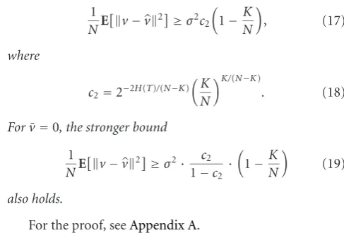
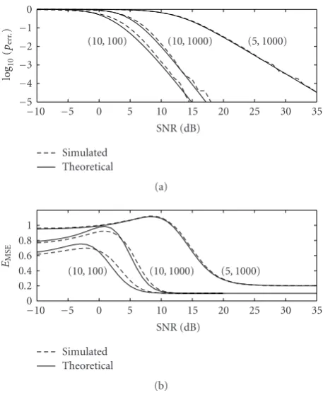
Figure6: Simulation of subspace selection error probability and normalized expected MSE for isotropic random dictionaries. Cal-culations were made for integer SNRs (in dB), with 5×10⁵ inde-pendent simulations per data point. In all cases,K=1. The curve pairs are labeled by (N,M). Simulation results are compared to the estimates from Theorems3and4.
For each integer SNR from−10 dB to 35 dB, the subspace se-lection and normalized MSE were measured for 5×10⁵ inde-pendent experiments. The resulting empirical probabilities of subspace selection error and normalized expected MSEs are shown inFigure 6. Plotted alongside the empirical results are the estimatesperrandEMSEfrom (30) and (36).
Comparing the theoretical and measured values in Figure 6, we see that the theoretical values match the sim-ulation closely over the entire SNR range. Also note that Figure 6b shows qualitatively the same behavior as Figures 2and3(the direction of the horizontal axis is reversed). In particular,EMSE ≈K/N for high SNR and the low-SNR be-havior depends onMandNas described by (22).
4.4. Asymptotic analysis
The estimatesperrandEMSEare not difficult to compute nu-merically, but the expressions (30) and (36) provide little di-rect insight. It is thus interesting to examine the asymptotic behavior of perr andEMSEasNandM grow. The following theorem gives an asymptotic expression for the limiting value of the error probability function.
Theorem 5. Consider the function perr(N,M,K,γ)defined in (30). Define the critical SNR as a function of M, N,
andKas
γcrit=C−1=
J−1 rβ(r,s)
1/r
−1, (38)
whereC,r,s, andJare defined in(32)and(33). ForK =1 and any fixedγandγcrit,
lim
N,M→∞
γcrit constant
perr(N,M,K,γ)= ⎧ ⎨ ⎩
1 ifγ < γcrit, 0 ifγ > γcrit,
(39)
where the limit is on any sequence ofMandNwithγcrit con-stant.
For the proof, seeAppendix D.
The theorem shows that, asymptotically, there is a criti-cal SNRγcrit above which the error probability goes to one and below which the probability is zero. Thus, even though the frame is random, the error event asymptotically becomes deterministic.
A similar result holds for the asymptotic MSE.
Theorem 6. Consider the functionEMSE(M,N,K,γ)defined in(36)and the critical SNRγcrit defined in(38). ForK =1 and any fixedγandγcrit,
lim
N,M→∞
γcrit constant
EMSE(M,N,K,γ)= ⎧ ⎨ ⎩
Elim(γ) ifγ < γcrit, 0 ifγ > γcrit,
(40)
where the limit is on any sequence ofMandNwithγcrit con-stant, and
Elim(γ)=γ +γcrit 1 +γcrit.
(41)
For the proof, seeAppendix E.
Remarks. (i) Theorems 5 and6 hold for any values of K. They are stated for K = 1 because the significance of
perr(N,M,K,γ) andEMSE(M,N,K,γ) is proven only forK= 1.
(ii) Both Theorems5and6involve limits withγcritconstant. It is useful to examine how M,N, andK must be related asymptotically for this condition to hold. One can use the definition of the beta function β(r,s) = Γ(r)Γ(s)/Γ(r +s) along with Stirling’s approximation, to show that whenK
N,
rβ(r,s)1/r≈1. (42)
Substituting (42) into (38), we see thatγcrit ≈J1/r−1. Also, forKNandKM,
J1/r=
M
K
2/(N−K)
≈
M
K 2K/N
101 100
10−1 10−2
SNR 0
0.2 0.4 0.6 0.8 1 1.2 1.4
No
rm
al
iz
ed
M
S
E
γcrit.=2
γcrit.=1
γcrit.=0.5
Figure7: Asymptotic normalized MSE asN → ∞(fromTheorem 6) for various critical SNRsγcrit.
so that
γcrit≈
M K
2K/N
−1 (44)
for smallKand largeMandN. Therefore, forγcritto be con-stant, (M/K)2K/N must be constant. Equivalently, the
dictio-nary sizeM must grow asK(1 +γcrit)N/(2K), which is expo-nential in the inverse sparsityN/K.
The asymptotic normalized MSE is plotted inFigure 7for various values of the critical SNRγcrit. Whenγ > γcrit, the normalized MSE is zero. This is expected: fromTheorem 5, whenγ > γcrit, the estimator will always pick the correct sub-space. We know that for a fixed subspace estimator, the nor-malized MSE isK/N. Thus, asN→ ∞, the normalized MSE approaches zero.
What is perhaps surprising is the behavior forγ < γcrit. In this regime, the normalized MSE actually increaseswith increasing SNR. At the critical level,γ=γcrit, the normalized MSE approaches its maximum value
maxElim= 2γcrit 1 +γcrit
. (45)
Whenγcrit >1, the limit of the normalized MSEElim(γ) sat-isfiesElim(γ) > 1. Consequently, the sparse approximation results in noiseamplificationinstead of noise reduction. In the worst case, asγcrit → ∞,Elim(γ)→ 2. Thus, sparse ap-proximation can result in a noise amplification by a factor as large as 2. Contrast this with the factor of 4 in (21), which seems to be a very weak bound.
5. COMMENTS AND CONCLUSIONS
This paper has addressed properties of denoising by sparse approximation that are geometric in that the signal model is membership in a specified union of subspaces, without a
probability density on that set. The denoised estimate is the feasible signal closest to the noisy observed signal.
The first main result (Theorems1and2) is a bound on the performance of sparse approximation applied to a Gaus-sian signal. This lower bound on mean-squared approxima-tion error is used to determine an upper bound on denoising MSE in the limit of low input SNR.
The remaining results apply to the expected perfor-mance when the dictionary itself is random with i.i.d. en-tries selected according to an isotropic distribution. Easy-to-compute estimates for the probability that the subspace con-taining the true signal is not selected and for the MSE are given (Theorems3and4). The accuracy of these estimates is verified through simulations. Unfortunately, these results are proven only for the case ofK = 1. The main technical difficulty in extending these results to generalK is that the distances to the various subspaces are not mutually indepen-dent. (ThoughLemma 2does not extend toK >1, we expect that a relation similar to (B.10) holds.)
Asymptotic analysis (N→ ∞) of the situation with a ran-dom dictionary reveals a critical value of the SNR (Theorems 5 and6). Below the critical SNR, the probability of select-ing the subspace containselect-ing the true signal approaches zero and the expected MSE approaches a constant with a simple, closed form; above the critical SNR, the probability of select-ing the subspace containselect-ing the true signal approaches one and the expected MSE approaches zero.
Sparsity with respect to a randomly generated dictionary is a strange model for naturally occurring signals. However, most indications are that a variety of dictionaries lead to performance that is qualitatively similar to that of random dictionaries. Also, sparsity with respect to randomly gener-ated dictionaries occurs when the dictionary elements are produced as the random instantiation of a communication channel. Both of these observations require further investi-gation.
APPENDIX
A. PROOF OF THEOREMS1AND2
We begin with a proof ofTheorem 2;Theorem 1will follow easily. The proof is based on analyzing an idealized encoder forv. Note that despite the idealization and use of source-coding theory, the bounds hold for any values of (N,M,K)— the results are not merely asymptotic. Readers unfamiliar with the basics of source-coding theory are referred to any standard text, such as [50–52], though the necessary facts are summarized below.
Consider the encoder forvshown in Figure 8. The en-coder operates by first finding the optimal sparse approx-imation ofv, which is denoted byv. The subspaces in ΦK
are assumed to be numbered, and the index of the subspace containingvis denoted byT.vis then quantized with a K-dimensional,b-bit quantizer represented by the box “Q” to produce the encoded version ofv, which is denoted byvQ.
v
H(T) bits bbits
SA
v
T Q vQ
Figure8: The proof ofTheorem 2is based on the analysis of a hy-pothetical encoder forv. The sparse approximation box “SA” finds the optimalK-sparse approximation ofv, denoted byv, by com-putingv=PTv. The subspace selectionTcan be represented with
H(T) bits. The quantizer box “Q” quantizes vwith bbits, with knowledge ofT. The overall output of the encoder is denoted by
vQ.
communicateTto a receiver that knows the probability mass function ofTis given by the entropy ofT, which is denoted byH(T) [51]. In analyzing the encoder forv, we assume that a large number of independent realizations ofvare encoded at once. This allowsbto be an arbitrary real number (rather than an integer) and allows the average number of bits used to representT to be arbitrarily close toH(T). The encoder ofFigure 8can thus be considered to useH(T) +b bits to representvapproximately asvQ.
The crux of the proof is to represent the squared error that we are interested in,v−v2, in terms of squared errors of the overall encoderv→vQand the quantizerv→vQ. We will show the orthogonality relationship below and bound both terms:
Ev−v2= E v−v Q 2
bounded below using fact (a)
− Ev−vQ2
bounded above using fact (b) .
(A.1) The two facts we need from rate-distortion theory are as fol-lows [50–52].
(a) The lowest possible per-component MSE for encoding an i.i.d. Gaussian source with per-component variance σ2withRbits per component isσ22−2R.
(b) Any source with per-component variance σ2 can be encoded with R bits per component to achieve per-component MSEσ22−2R.
(The combination of facts (a) and (b) tells us that Gaussian sources are the hardest to represent when distortion is mea-sured by MSE.)
Applying fact (a) to thev→vQencoding, we get 1
NE v−vQ 2
≥σ22−2(H(T)+b)/N. (A.2)
Now we would like to define the quantizer “Q” inFigure 8to get the smallest possible upper bound onE[v−vQ2].
Since the distribution ofvdoes not have a simple form (e.g., it is not Gaussian), we have no better tool than fact (b), which requires us only to find (or upper bound) the variance
of the input to a quantizer. Consider a two-stage quantiza-tion process forv. The first stage (with access toT) applies an affine, length-preserving transformation tovsuch that the result has zero mean and lies in aK-dimensional space. The output of the first stage is passed to an optimal b-bit quantizer. Using fact (b), the performance of such a quan-tizer must satisfy
1
KE v−vQ 2
≤σv2|T2−2b/K, (A.3)
whereσ2
v|T is the per-component conditional variance ofv,
in theK-dimensional space, conditioned onT.
From here on, we have slightly different reasoning for the ¯
v=0 and ¯v=0 cases. For ¯v=0, we get an exact expression for the desired conditional variance; for ¯v = 0, we use an upper bound.
When ¯v = 0, symmetry dictates thatE[v | T] = 0 for allTandE[v]=0. Thus, the conditional varianceσ2
v|T and
unconditional varianceσ2
v are equal. Taking the expectation
of
v2= v2+v−v2 (A.4) gives
Nσ2=Kσ2
v+E
v−v2. (A.5) Thus
σ2
v|T =σv2=
1 K
Nσ2−Ev−v2=N K
σ2−D SA
, (A.6) where we have usedDSAto denote (1/N)E[v−v2]—which is the quantity we are bounding in the theorem. Substituting (A.6) into (A.3) now gives
1
KE v−vQ 2
≤N
σ2−D
SA
K 2
−2b/K. (A.7)
To usefully combine (A.2) and (A.7), we need one more orthogonality fact. Since the quantizer Q operates in sub-spaceT, its quantization error is also in subspaceT. On the other hand, becausevis produced by orthogonal projection to subspaceT,v−vis orthogonal to subspaceT. So
v−vQ 2
= v−vQ 2+v−v2. (A.8) Taking expectations, rearranging, and substituting (A.2) and (A.7) gives
Ev−v2=E v−v Q
2
−E v−vQ 2
≥Nσ22−2(H(T)+b)/N−Nσ2−DSA
2−2b/K. (A.9) Recalling that the left-hand side of (A.9) isNDSAand rear-ranging gives
DSA≥σ2
2−2(H(T)+b)/N−2−2b/K
1−2−2b/K
Since this bound must be true for allb ≥0, one can max-imize with respect tobto obtain the strongest bound. This maximization is messy; however, maximizing the numerator is easier and gives almost as strong a bound. The numerator is maximized when
b= K
N−K
H(T) +N 2 log2
N K
, (A.11)
and substituting this value ofbin (A.10) gives
DSA≥σ2·
2−2H(T)/(N−K)(1−(K/N))(K/N)K/(N−K) 1−2−2H(T)/(N−K)(K/N)N/(N−K) .
(A.12) We have now completed the proof ofTheorem 2for ¯v=0.
For ¯v=0, there is no simple expression forσ2
v|Tthat does
not depend on the geometry of the dictionary, such as (A.6), to use in (A.3). Instead, use
σv2|T ≤σv2≤
N Kσ
2, (A.13)
where the first inequality holds because conditioning cannot increase variance and the second follows from the fact that the orthogonal projection ofvcannot increase its variance, even if the choice of projection depends onv. Now following the same steps as for the ¯v=0 case yields
DSA≥σ2
2−2(H(T)+b)/N−2−2b/K (A.14)
in place of (A.10). The bound is optimized overbto obtain
DSA≥σ2·2−2H(T)/(N−K)
1−
K N
K N
K/(N−K) .
(A.15) The proof ofTheorem 1now follows directly: sinceTis a discrete random variable that can take at mostJ values, H(T)≤log2J.
B. PROOF OFTHEOREM 3
Using the notation ofSection 4.1, letVj, j = 1, 2,. . .,J, be
the subspaces spanned by theJ possibleK-element subsets of the dictionaryΦ. LetPj be the projection operator onto
Vj, and letTbe index of the subspace closest toy. Let jtrue be the index of the subspace containing the true signalx, so that the probability of error is
perr=Pr
T=jtrue
. (B.1)
For eachj, letxj=Pjy, so that the estimatorxSAin (26) can be rewritten asxSA=xT. Also, define random variables
ρj=
y−xj 2
y2 , j=1, 2,. . .,J, (B.2) to represent the normalized distances betweenyand theVj’s.
Henceforth, theρj’s will be calledangles, sinceρj =sin2θj,
whereθjis the angle betweenyandVj. The angles are well
defined sincey2>0 with probability one.
Lemma 1. For all j = jtrue, the angleρj is independent ofx
andd.
Proof. Given a subspaceVand vectory, define the function
R(y,V)= y−PVy
2
y2 , (B.3) where PV is the projection operator onto the subspace y.
Thus,R(y,V) is the angle betweenyandV. With this no-tation,ρj =R(y,Vj). Sinceρjis a deterministic function of
yandVjandy=x+d, to showρjis independent ofxandd,
it suffices to prove thatρjis independent ofy. Equivalently,
we need to show that for any functionG(ρ) and vectorsy0 andy1,
EGρj
|y=y0
=EGρj
|y=y1
. (B.4) This property can be proven with the following symmetry argument. LetUbe any orthogonal transformation. SinceU is orthogonal,PUV(U y) = UPVy for all subspacesV and
vectorsy. Combining this with the fact thatUv = vfor allv, we see that
R(U y,UV)= U y−PUV(U y)
2
U y2 = U
y−PV(y) 2
U y2
= y−PV(y)
2
y2 =R(y,V).
(B.5) Also, for any scalarα >0, it can be verified thatR(αy,V)=
R(y,V).
Now, lety0andy1be any two possible nonzero values for the vectory. Then, there exist an orthogonal transformation Uand scalarα >0 such thaty1=αU y0. Since j= jtrueand K=1, the subspaceVjis spanned by vectorsϕi, independent
of the vectory. Therefore, EGρj
|y=y1
=EGRy1,Vj
=EGRαU y0,Vj
=EGRU y0,Vj
.
(B.6) Now since the elements ofΦare distributed uniformly on the unit sphere, the subspaceUVj is identically distributed
toVj. Combining this with (B.5) and (B.6),
EGρj
|y=y1
=EGRU y0,Vj
=EGRU y0,UVj
=EGRy0,Vj
=EGρj
|y=y0
,
(B.7)
and this completes the proof.
Lemma 2. The random anglesρj,j= jtrue, are i.i.d., each with
a probability density function given by the beta distribution
pρ(ρ)= 1
β(r,s)ρ
r−1(1−ρ)s−1, 0≤ρ≤1, (B.8)
Proof. SinceK =1, each of the subspacesVjfor j = jtrueis spanned by a single, unique vector inΦ. Since the vectors in
Φare independent and the random variablesρjare the angles
betweenyand the spacesVj, the angles are independent.
Now consider a single angleρjforj=jtrue. The angleρj
is the angle betweenyand a random subspaceVj. Since the
distribution of the random vectors definingVjis spherically
symmetric andρj is independent of y,ρj is identically
dis-tributed to the angle between any fixed subspaceVand a ran-dom vectorzuniformly distributed on the unit sphere. One way to create such a random vectorzis to takez=w/w, wherew ∼N(0,IN). Letw1,w2,. . .,wK be the components
ofwinV, and letwK+1,wK+2,. . .,wN be the components in
the orthogonal complement toV. If we define
X=
K
i=1 w2
i, Y = N
i=K+1 w2
i, (B.9)
then the angle betweenzandVisρ=Y/(X+Y). SinceXand Y are the sums ofKandN−Ki.i.d. squared Gaussian ran-dom variables, they are Chi-squared ranran-dom variables with K andN−K degrees of freedom, respectively [53]. Now, a well-known property of Chi-squared random variables is that if X andY are Chi-squared random variables withm andndegrees of freedom,Y/(X+Y) will have the beta dis-tribution with parametersm/2 andn/2. Thus,ρ=Y/(X+Y) has the beta distribution, with parametersrandsdefined in (33). The probability density function for the beta distribu-tion is given in (B.8).
Lemma 3. Letρmin=minj=jtrueρj. Thenρminis independent
ofxanddand has the approximate distribution
Prρmin>
≈exp−(C)r (B.10)
for small, whereCis given in(32). More precisely, Prρmin>
<exp−(C)r(1−)s−1 for all∈(0, 1), Prρmin>
>exp
− (C)r
(1−)
for0<rβ(r,s)1/(r−1). (B.11) Proof. SinceLemma 1shows that eachρjis independent ofx
andd, it follows thatρminis independent ofxanddas well. Also, for anyj=jtrue, by bounding the integrand of
Prρj<
= 1
β(r,s)
0 ρ
r−1(1−ρ)s−1dρ (B.12)
from above and below, we obtain the bounds (1−)s−1
β(r,s)
0ρ
r−1dρ <Prρ
j<
< 1
β(r,s)
0ρ
r−1dρ, (B.13) which simplify to
(1−)s−1r
rβ(r,s) <Pr
ρj<
<
r
rβ(r,s). (B.14)
Now, there are J −1 subspaces Vj where j = jtrue, and by Lemma 2, the ρj’s are mutually independent.
Con-sequently, if we apply the upper bound of (B.14) and 1−δ > exp(−δ/(1−δ)) forδ ∈ (0, 1), withδ = r/(rβ(r,s)), we
obtain Prρmin>
=
j=jtrue
Prρj>
>
1− r
rβ(r,s) J−1
>exp
− r(J−1)
rβ(r,s)(1−δ)
for 0<<(rβ(r,s))1/r,
>exp
− r(J−1)
rβ(r,s)(1−)
for 0<<rβ(r,s)1/(r−1). (B.15) Similarly, using the lower bound of (B.14), we obtain
Prρmin>
=
j=jtrue
Prρj>
<
1−(1−)s−1r
rβ(r,s) J−1
<exp
−(1−)s−1r(J−1)
rβ(r,s)
.
(B.16)
Proof ofTheorem 3.LetVtrue be the “correct” subspace, that is,Vtrue =Vjforj = jtrue. LetDtruebe the squared distance fromytoVtrue, and letDminbe the minimum of the squared distances from yto the “incorrect” subspacesVj, j = jtrue. Since the estimator selects the closest subspace, there is an error if and only ifDmin≤Dtrue. Thus,
perr=Pr
Dmin≤Dtrue
. (B.17)
To estimate this quantity, we will approximate the probability distributions ofDminandDtrue.
First considerDtrue. Write the noise vectordasd=d0+ d1, whered0is the component inVtrueandd1is inVtrue⊥ . Let D0= d02andD1= d12. Sincey=x+dandx∈Vtrue, the squared distance fromytoVtrueisD1. Thus,
Dtrue=D1. (B.18) Now considerDmin. For any j,xj is the projection of y
ontoVj. Thus, the squared distance fromyto any spaceVj
isy−xj2=ρjy2. Hence, the minimum of the squared
distances fromyto the spacesVj,j=jtrue, is
Dmin=ρminy2. (B.19) We will bound and approximatey2 to obtain the bound and approximation of the theorem. Notice that y=x+d=
x+d0+d1, wherex+d0∈Vtrueandd1∈Vtrue⊥ . Using this or-thogonality and the triangle inequality, we obtain the bound
y2= x+d
0 2+ d1 2≥
x − d0 2+ d1 2
=N−D0 2
+D1.