On the Fixation Process of a Beneficial Mutation in a Variable Environment

(1)

INVESTIGATION

On the Fixation Process of a Bene

ﬁ

cial Mutation

in a Variable Environment

Hildegard Uecker1_{and Joachim Hermisson} Mathematics and Biosciences Group, Faculty of Mathematics and Max F. Perutz Laboratories, University of Vienna, A-1090 Vienna, Austria

ABSTRACTA population that adapts to gradual environmental change will typically experience temporal variation in its population size and the selection pressure. On the basis of the mathematical theory of inhomogeneous branching processes, we present a framework to describe thefixation process of a single beneficial allele under these conditions. The approach allows for arbitrary time-dependence of the selection coefficients(t) and the population sizeN(t), as may result from an underlying ecological model. We derive compact analytical approximations for thefixation probability and the distribution of passage times for the beneficial allele to reach a given intermediate frequency. We apply the formalism to several biologically relevant scenarios, such as linear or cyclic changes in the selection coefficient, and logistic population growth. Comparison with computer simulations shows that the analytical results are accurate for a large parameter range, as long as selection is not very weak.

F

OR adaptive evolution to proceed, it is not enough that new beneficial mutations enter a population. To com-plete an adaptive step, these mutations also need to escape stochastic loss due to genetic drift, get established, and fi -nally rise to fixation. Thefixation process of beneficial (or neutral or deleterious) alleles is one of the building blocks of population genetic theory and many of the key results on

ﬁxation probabilities and times date back to its early days. Two alternative mathematical frameworks have been devel-oped to derive analytical expressions for these quantities: branching processes (Fisher 1922, 1930; Haldane 1927) and diffusion theory (Kimura 1962; Kimura and Ohta 1969). Today, a large body of literature exists to studyﬁ x-ation under various ecological scenarios and genetic condi-tions (reviewed in Patwa and Wahl 2008), such as the effects of population structure (Whitlock 2003) and spatial heterogeneity (Whitlock and Gomulkiewicz 2005) and in-terference due to selection on linked loci (Barton 1995) or due to epistatic interaction (Takahasi and Tajima 2005).

In this article, we consider thefixation process in a variable environment, leading to time-dependent selection coefficients and population sizes. Aspects of this problem have already been studied in previous work: In particular, the impact of various scenarios of demographic change (growth, decline, cycles) on thefixation probability has been treated in a series of articles (Ewens 1967; Chia 1968; Kimura and Ohta 1974; Otto and Whitlock 1997; Pollak 2000; Parsons and Quince 2007a; Orr and Unckless 2008). Studies on time-dependent selection mostly concentrate on stochasticfluctuations of the selection coefficient (Jensen 1973; Karlin and Levikson 1974; Takahata and Ishii 1975; Huillet 2011). Since the distribution of the selection coefficients is constant across generations, these models are still time-homogeneous in a probabilistic sense. In contrast, surprisingly little is known when the changes of the selection coefficients=s(t) follow an explicit trend. Ohta and Kojima (1968) derive an expression for the

ﬁxation probability of a mutation with time-dependent selec-tive advantage in the context of the evolution of chromo-somal inversions. Apart from that, only particular functions have been considered: Kimura and Ohta (1969) discuss the case where selection decreases exponentially in time, and Pollak (1966) derives expressions for theﬁxation probability under two alternating selection pressures. No previous work seems to exist where both population size and selection strength are variable, although this is a generic case under realistic ecological conditions. Also, there does not seem to be

Manuscript received February 17, 2011; accepted for publication May 17, 2011 Supporting information is available online at http://www.genetics.org/content/ suppl/2011/06/06/genetics.110.124297.DC1.

1_{Corresponding author: Mathematics and Biosciences Group, Faculty of Mathematics,}

(2)

an investigation of ﬁxation or passage times in variable environments.

In the following, we present a formalism to describe the

fixation process under a wide range of scenarios of environ-mental variation. We use branching processes in continuous time to derive analytical approximations for the fixation probability and the passage time needed for the mutant allele to reach some intermediate frequency xc. After the introduction of our model, we describe how a general ap-proximation for the fixation probability can be obtained from known mathematical results on inhomogeneous branching processes. Afterward, we discuss applications of this result to several biologically relevant scenarios. In the second part of the article, we introduce and apply a method to calculate the distribution of the passage time needed for a beneficial mutation to reach an intermediate frequency. The method works by combining the stochasticfluctuations from the branching approximation with the deterministic growth of the full model. This technique has been used before (for constant selection and population size) by Desai and Fisher (2007) in a model of clonal evolution. All ana-lytical results are complemented by computer simulations, which are briefly described in a separate section. We close with a short discussion. In theAppendix, we discuss a gener-alized version of the model to include allele-frequency– dependent population demographies. We illustrate how the formalism can be used by applying it to an illustrative ecological scenario: thefixation probability of a“rescue mu-tation”in a population that is threatened by extinction (cf. Orr and Unckless 2008). Additional material is devoted to

Supporting Information,File S1,Figure S1,Figure S2, and

Figure S3. We discuss in some detail the scope and limits of the approach and the accuracy of the approximation. In section S2 of File S1, we present an alternative treatment to derive theﬁxation probability in a variable environment from a diffusion approach.

The Model

We consider a large population of haploid individuals with time-dependent population sizeNt. The population dynam-ics are modeled as a time-inhomogeneous birth–death pro-cess with birth and death ratesb(t,Nt) andd(t,Nt):

Nt/Ntþ1: bðt;NtÞNt;

Nt/Nt21: dðt;NtÞNt: (1)

The impact of the changes in the external environment on the population size is reﬂected in the explicit time-dependence of the rates ont. The dependence onNtaccounts for density-dependence [e.g., logistic: bðt;NtÞ ¼ b1ðtÞ2b2ðtÞNt]. We call rðt;NtÞ ¼ bðt;NtÞ2dðt;NtÞ the growth parameter. Obviously, the expected change ofNtover a small time interval dtreads

E½DNjNt ¼rðt;NtÞNtdt: (2)

Consider now two alleles, a beneﬁcial mutant allele A

and the ancestral (resident) allele a, that segregate in the population at a single locus. Recurrent mutations in both directions are ignored. In general, birth and death rates might be different for residents and mutants. These rates can depend on time and on the (absolute) frequencies of both allelic types, allowing for general frequency-dependent selection. As a consequence, also the population dynamics depend on the allelic composition and cannot be described by Equation 1 anymore. We discuss this model in the Appen-dix. For the main part of the article, however, we assume that the rates are the same for mutants and residents and that all model parameters are independent of allele frequen-cies. This means in particular that selection is soft; i.e., changes in the allelic composition due to selection or drift do not interfere with the population dynamics. Population growth and decline of the polymorphic population are then correctly described by Equation 1.

In this setting, selection is modeled as competitive replacement between individuals, which does not change the population size, and is implemented as follows: At per capita rate j(t,Nt) +s(t,Nt), a mutant additionally repro-duces and succeeds in replacing a randomly chosen indi-vidual from the population by its offspring. Residents do the same at ratej(t,Nt). Again, the selective advantage

s(t, Nt) of the mutant may thus depend on the external environment (modeled by the dependence of s(t, Nt) on

t) and the population size (modeled by the dependence on Nt). Changes in the number of mutants then occur at rates

nt/ntþ1: ðjðt;NtÞ þsðt;NtÞÞntðNNt2t ntÞþbðt;NtÞnt; nt/nt21: jðt;NtÞntðN_Nt2_t ntÞþdðt;NtÞnt:

(3)

The model corresponds to a continuous-time Moran model, but with a population size that may change in time. Putting b(t,Nt) =d(t,Nt) = 0,j(t,Nt) = 1, ands(t,Nt) =

s = const. reproduces the standard Moran model (Moran 1958a,b; Novozhilov et al. 2006). The free parameter

j(t,Nt) has been introduced to our model to allow for easy interpolation to other models (see below) and additionally to make the analysis of density-dependent competition possible.

To further clarify the relation to other models, we calculate how the frequency of mutantsxt:=nt/Ntchanges over time. Let Dxbe its change in an inﬁnitesimal time in-terval dt. The expectation and the variance ofDxare calcu-lated to be

E½Dxjxt;Nt ¼sðt;NtÞxtð12xtÞdt; (4a)

Var½Dxjxt;Nt E h

ðDxÞ2jxt;Nt i

xtð12xtÞ

(3)

with the time-dependent variance effective population size

Ne;t¼ Nt

2jðt;NtÞ þbðt;NtÞ þdðt;NtÞ þsðt;NtÞ: (5)

In the last step we approximatedNt+ 1NtandNt21

Nt(see section S3 ofFile S1for the derivation of Equations 4a and 4b).

We see that the strength of drift, measured as N21 e;t, is proportional to the total rate of events in the model. The choice 2jðt; NtÞ þbðt; NtÞ þdðt; NtÞ ¼2 coincides with the strength of drift in the standard Moran model, while 2jðt; NtÞ þbðt; NtÞ þdðt; NtÞ ¼1 is consistent with the scal-ing in the Wright–Fisher model. In contrast to many diffu-sion or coalescent approaches, we do not rescale time with the effective population size (which would be impractical sinceNe;t itself depends ont). Generation time in the con-tinuous-time Moran model is deﬁned as the inverse of the total death rate of an individual,ðjðt;NtÞ þdðt;NtÞÞ21, and

may again depend on time in our model.

Fixation Probability

Analytical theory

Following pioneering work by Haldane (1927) and Fisher (1930), there has been a long tradition in population genet-ics to calculate ﬁxation probabilities by branching process methods (reviewed in Haccou et al.2005 and Patwa and Wahl 2008). For the general time-dependent case, the rele-vant results have long been known in the mathematical literature (e.g., Kendall 1948; Allen 2011). However, only speciﬁc cases (usually in the context of changing population sizes) have been discussed in the population genetics con-text (Ewens 1967; Otto and Whitlock 1997; Pollak 2000; Wahl and Gerrish 2001). We therefore give a brief outline of the general theory below and show how it applies to the biological problem at hand. Previous results are recovered as special cases.

The branching process approximation is based on the following reasoning: Initially, the fate of a new beneficial mutation arising in a population will be strongly determined by genetic drift. In most cases it will actually get lost again. Once the mutation has survived this early phase, it is, however, almost sure to get fixed given its selective ad-vantage is large enough. To calculate thefixation probability it is therefore often sufficient to consider the stage at which the mutant population size nt is still small relative to the total population size Nt. In this early phase, the mutant individuals suffer nearly independent fates, as do the indi-viduals in a Galton–Watson branching process (this as-sumption is precisely met in an infinite population). The extinction probability of the latter can therefore be used as an approximation for the probability that the mutation gets lost. Because a mutation in afinite population is in the long term eitherfixed or lost, thefixation probability is the com-plementary probability. (We exclude the unbiological case of

a population that increases without bounds, where possibly neither wild types nor mutants become extinct.)

Ignoring terms proportional to xt = nt/Nt in the birth– death model (Equation 3), which corresponds to the limit

Nt/N, leads to transition rates that are proportional tont. Following standard practice in ecological modeling, we fur-ther ignore stochasticﬂuctuations in the population dynam-ics. This is done by replacing the stochastic variableNtby its deterministic approximation denoted asN(t), with dynamics

dNðtÞ

dt ¼rðt;NðtÞÞNðtÞ: (6)

Inserting the deterministic solution N(t) into the rates for birth, death, and selection reduces the dependence of these rates on t and Nt to a dependence on t only [sðt; NtÞ/sðt; NðtÞÞ ¼:sðtÞ, etc.]. We arrive at a branching process with time-dependent per capita birth and death rates:

birth rate : lðtÞ ¼bðtÞ þjðtÞ þsðtÞ;

death rate : mðtÞ ¼dðtÞ þjðtÞ: (7)

As explained above for the birth–death process, the total rate of events determines the strength of genetic drift, while

l(t)2m(t) =s(t) +r(t) corresponds to the absolute ex-pected rate of increase of a small mutant population (its Malthusianﬁtness parameter).

To derive the extinction probability of this process, we follow Allen (2011, p. 278ff). Letpi(n0,t) be the probability that there areiindividuals at timetwhen the process started with n0 individuals at time t = 0. Using the Kolmogorov forward equation,

dpiðn0;tÞ

dt ¼lðtÞði21Þpi21ðn0;tÞ þmðtÞðiþ1Þpiþ1ðn0;tÞ 2 ðlðtÞ þmðtÞÞipiðn0;tÞ;

(8)

a differential equation for the probability generating func-tion Pn0ðz;tÞ ¼

P_N

i¼0piðn0;tÞzi of the branching process can be derived (see Allen 2011, p. 279):

@Pn0ðz;tÞ @t ¼

lðtÞz22zþmðtÞð12zÞ@Pn0ðz;tÞ @z ;

Pn0ðz;0Þ ¼z n0:

(9)

The solution is known from the mathematical literature (Kendall 1948; Allen 2011, p. 280) and given as

Pn0ðz;tÞ ¼

1þ 1

e2rðtÞ_=ð_z₂₁_Þ₂Ðt

0lðtÞe2rðtÞdt

n0

(10)

with

rðtÞ ¼ðt

0½lðtÞ2mðtÞdt¼ ð_t

(4)

To keep notation short, we introduce the abbreviations

AðtÞ:¼e2rðtÞ; (12a)

BðtÞ:¼ ðt

0

lðtÞe2rðtÞdt: (12b)

The extinction probability p0(n0,t) is immediately ob-tained from the generating function via

p0ðn0;tÞ ¼Pn0ð0;tÞ ¼

12 1

ðAþBÞðtÞ

n0

¼ Ðt

0mðtÞe 2rðtÞ_dt

1þÐ₀tmðtÞe2rðtÞ_dt n0

: (13)

The probability that the mutation will eventually ﬁx in the population is therefore given by

pfixðn0Þ ¼12 lim

t/Np0ðn0; tÞ ¼12

12 1

AþB n0

; (14)

where we introduced

AþB¼lim

t/NðAþBÞðtÞ ¼1þ ð_N

0

mðtÞe2rðtÞdt

¼ ð_N

0

lðtÞe2rðtÞdt: (15)

The last equality is valid for limt/Nexpð2rðtÞÞ ¼0. This condition is met in all examples considered below. For a sin-gle mutant (n0= 1), it thus holds:

pfix¼ 1

AþB¼

2

h

1þÐN₀ðlþmÞðtÞexp

2Ðt

0ðsþrÞðtÞdt dt

i

(16a)

¼h 2

1þÐN₀ ðNð0Þ= NeðtÞÞexp

2Ðt

0sðtÞdt dt

i;

(16b)

where we have usedÐ₀trðtÞdt¼Ð₀tðN_ðtÞ= NðtÞÞdt¼lnðNðtÞ=Nð0ÞÞ for the last equality and Ne(t) is deﬁned analogously to Equation 5. A similar expression was also derived by Ohta and Kojima (1968). Restricted to a constant population size and a Poisson offspring distribution, their result is, how-ever, less general.

The result depends on two independent parameters, which are compositions of three biologically relevant fac-tors: the strength of selection given by s(t), the combined rate of birth and death events (l+m)(t), and the changes in the total population size [modeled byr(t) orN(t)]. In the above equation we formulated the result via two different combinations of these three variables. In the ﬁrst version (Equation 16a) it is expressed in terms of the absolute rate

of increase of mutants in the population (s+r)(t) and the total rate (l+m)(t) at which events happen, which defines the time scale of the problem and also quantifies the infl u-ence of drift. In the second formulation (Equation 16b) of the result we combined the birth and death rates and the changing population size with the time-dependent vari-ance effective population size. The second decisive param-eter is the selection coefficient of the mutation. Depending on the question to be answered, one or the other version is more favorable. In the first version, the correspondence between a mutation with time-dependent selective advan-tage and a mutation in a population of changing size can be easily seen: a mutation with time-dependent selective advantage s(t) in a population of (on average) constant size b(t) = d(t) = const. has the same chance to reach

ﬁxation as a mutation with constant selective advantage

s0 in a population with time-dependent death rate d(t) and growth parameter r(t) = s(t)2 s0. [Note, however, that s0must be .0, such that ﬁxation is (almost) certain once the mutation has survived genetic drift.] The second version is closer to the traditional view in population ge-netics. It is advantageous if the variance effective popula-tion size is directly given and allows, in particular, also for the treatment of discontinuous changes in the population size.

We see that the ﬁxation probability is independent of many details of the individual-level dynamics of the original process (Equation 3), which depends on four rates [b(t,Nt),

d(t, Nt), s(t, Nt), and j(t,Nt)]. Further aspects of the sto-chastic model are ignored by our deterministic approxima-tion for the populaapproxima-tion dynamics. In particular, the analytical results become independent of the particular form of density regulation. As an example, consider three scenarios: (1) a population with inherently constant size N0withb(t,Nt) =

d(t,Nt) = 0 andj(t,Nt) =c; (2) a population with den-sity regulation according to bðt; NtÞ ¼cþrð12Nt=N0Þ and d(t, Nt)¼c, with initial size N0, and j(t, Nt) = 0; and (3) a population without density regulation with

bðt;NtÞ ¼dðt;NtÞ ¼c, initial size N0, and j(t,Nt) = 0. In all three cases, the deterministic dynamics of the population size are the same (N(t) =N0) and the analytical predictions for the fixation probability coincide for arbitrary s(t, Nt). Simulation results of all three scenarios indeed showed no significant difference, justifying the approximation (see sec-tion S1 ofFile S1). This observation agrees withfindings by Parsons and Quince (2007a) that demographic stochasticity does not significantly influence the fixation probability of advantageous alleles [Parsons and Quince (2007a) discuss this issue for a population that starts in the vicinity of the dynamic equilibrium]. For concreteness, we use the notion of“constant population size”in the following to refer to the case of a strictly constant population size ðbðt;NtÞ ¼

dðt;NtÞ ¼0Þ. We further setj(t) =j= const. in all appli-cations. If not stated otherwise, we usej=1 (corresponding to the Moran model scaling) for the results shown in the

(5)

A necessary condition for the branching approximation to yield meaningful results is that the fate of the mutation is decided as long as the mutant frequency xt =nt/Nt is still small. Asxtincreases, mutants are no longer independent in the original birth–death process (Equation 3), and both pro-cesses differ significantly from each other. In particular, the birth–death process has a second absorbing boundary atxt= 1. As a consequence, neutral or even deleterious mutations, too, can becomefixed by genetic drift. In the corresponding branching model, an upper absorbing boundary does not exist. Consequently, neutral or deleterious alleles must go extinct in the long term. For an allele with a general time-dependent selection coefficient, the branching process ap-proximation is thereby valid only if the allele is“sufficiently beneficial on average.” We can formalize this condition as follows: Since divergence of the (first) integral in Equation 15 leads to the wrong prediction of a zerofixation probabil-ity, we need to require that the integral converges. If we assume that m(t) is bounded below by a constantCm.0,

a necessary condition for the convergence of the integral is divergence of the integral in Equation 11. More precisely, if we assume thatm(t) has boundsCm.0,Cmsuch thatCm, m(t) , Cm, it must hold that limt/NrðtÞ.Cln½t for some constantC.1. A prominent example where this condition is not fulfilled is a mutation with an exponentially decreas-ing selection coefficient in a population of constant size [Kimura and Ohta (1969), cf. also Pollak (1966) and Ohta and Kojima (1968) for mutations that lose their advantage over time]. The condition is, however, not sufficient to ob-tain good results: It is also necessary that the contribution of times beyond the initial phase be negligible. In particular, changes in the environment at times larger than thefixation time must not have an impact on the results. As shown in section S1 of File S1, the approximation will usually be excellent if the estimate of pfix from Equation 16 fulfills

pfixN≳10. By a similar reasoning it is clear that the require-ment that the mutation be beneﬁcial all the time is at this point unnecessarily strict. It is sufﬁcient that the extinction probability is in both processes—the original birth–death process and the branching approximation—negligible once the number of mutants has reached a certain size.

Applications

Constant selection and constant population size: Setting

l(t) =j+sandm(t) =jyields for theﬁxation probability

pfix¼

s jþs

s j2s

Ne

N: (17)

The well-known result found by Haldane (1927) is there-fore reproduced forNe=N. In the special case of a constant environment, it is possible to calculate the exact ﬁxation probability from the transition matrix deﬁned via Equation 3 (see Ewens 2004, p. 90). One obtains

pð_fixexactÞ¼ ðs=ðjþsÞÞ

12ðj=ðjþsÞÞN

ðs=ðjþsÞÞ

12expð2ðs=ðjþsÞÞNÞ; (18)

which shows that the branching approximation is very accurate for large values ofsN/j. Furthermore, it is possible to calculate thefixation probability of a deleterious mutation with selective disadvantage 2s. To do so, we switch the roles of the transition rates defined in Equation 3. Every path leading to fixationn=Nhas now a chance to be re-alized, which is by a factor of (j + s)2N _{lower than the} corresponding path for a beneficial mutation. It immediately follows that

pfixð2sÞ ¼

pfixðsÞ

ðjþsÞN pfixðsÞ

expðsNÞ: (19)

Constant selection and changing population size:Otto and Whitlock (1997) analyzed thefixation probability for several important scenarios of demographic change. Our general result (Equation 16b) contains all those scenarios, among arbitrary others. In addition, it provides some insight into the influence of the individual-level dynamics on thefixation probability. As an example, we consider a population that follows logistic growth (or decline) until it has reached its new carrying capacity K. There are different ways to de-scribe these global dynamics at the individual level. We discuss two possibilities, which arise naturally in a biological context: Thefirst one assumes that a decreasing availability of resources per individual leads to a lower birth rate while the death rate stays constant (e.g., fertility is reduced). The second one assumes that the same circumstances lead to a higher death rate while the birth rate stays constant. The selection coefficient s of the beneficial mutant is con-stant in both cases. In thefirst scenario, the birth and death rates are given by

bðt;NtÞ ¼bþr

12Nt K ;

dðt;NtÞ ¼b:

(20)

The total population size thus changes according to

NðtÞ ¼ KN0

ðK2N0Þe2rtþN0; (21)

and using Equation 16b yields

pð_fix1Þ¼ sðrþsÞ

sðsþrÞ þ ðbþjÞðsþrg0Þ

(22)

with g0 ¼N0= K.

In the second scenario, birth and death rates are then given by

bðt;NtÞ ¼bþr;

dðt;NtÞ ¼bþrN_Kt:

(6)

While the deterministic dynamics at the population level are the same for both scenarios (given by Equation 21), this is not true for theﬁxation probability. From Equation 16b, we obtain for theﬁxation probability in the second scenario

pð_fix2Þ¼ sðrþsÞ

sðrþsÞ þ ðbþjÞðsþrg0Þ þg0rðrþsÞ

#pð_fix1Þ;

(24)

i.e., a reduced probability relative to the ﬁrst scenario. This is explained by the fact that genetic drift is stronger in the second scenario. For small values of s and r both

ﬁxation probabilities are approximately the same,

pð_fix1Þpð_fix2ÞsðrþsÞ=½ðbþjÞðsþrg0Þ; and reproduce the result found by Otto and Whitlock (1997) if we choose

b + j = 0.5 such that the variance of the increase in the mutant number Var[Dn|nt] is the same as in their model.

Note that for a sudden jump in population size, the result of our theory coincides with the result derived by Otto and Whitlock (1997) (where selection is effective during the change in population size), while Wahl and Gerrish (2001) consider a slightly different situation (where selec-tion is switched off during the bottleneck; cf. Patwa and Wahl 2008).

Linearly increasing selection: When environmental condi-tions develop continuously in a given direction, the selective advantage of a mutation may gradually increase during the

fixation process. Let us assume that the total population size stays constant and that the selection coefficient of the mutation linearly increases in time, thus s(t) = s0 + s1t. We obtain the following expression forpfixfrom Equation 16a,

pfix¼

1þj

ffiffiffiffiffiffiffiffi_p

2s1

r

es20=2s1_erfc

s0

ffiffiffiffiffiffiffi

2s1

p

₂1

; (25)

where erfcðxÞ ¼ ð2=pÞÐNx e2t

2

dtis the complementary error function. For the special cases0= 0, the result simpliﬁes,

pfixðs0¼0Þ ¼

1þj

ffiffiffiffiffiffiffi_p

2s1

r 21

ffiffiffiffi s1

p j

ffiffiffiffi

2

p r

: (26)

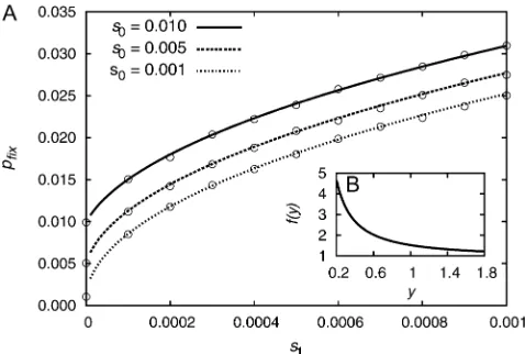
In Figure 1 the analytical results are compared to simu-lation results, showing very good agreement. The ﬁxation probability increases signiﬁcantly withs1. Generally,

pfixðsðtÞ ¼s0þs1tÞ

pfixðsðtÞ ¼s0Þ ¼

jþs0

s0þj

ffiffiffiffiffiffiffiffiffiffiffiffiffiffiffiffiffiffiffiffi ðps2

0=2s1Þ

q

es2

0=2s1_erfcð_s

0=

ffiffiffiffiffiffiffi

2s1

p Þ

h ffiffiffip

2

p

yey2=2erfc

y_ﬃﬃ

2

p i21_¼_:fðyÞ

(27)

with y:¼s0=pffiffiffiffis1. The functionf(y) is shown in the inset of Figure 1. Fory= 1 it is evaluated to bef(1) 1.52. This

means that ify1,i.e.,s0 pffiffiffiffis1, we observe an increase in thefixation probability of50% in comparison to a muta-tion with constant selective advantage. E.g., for initially moderately strong selections0¼0:01 thefixation probabil-ity is still increased by50% if selection increases as slightly ass(t) = 0.01 + 0.0001t.

Periodically changing selection: Cyclic environmental changes, such as seasonal changes or cyclic climate

ﬂuctuations (like the El Niño phenomenon), are frequent in nature. In the following, we consider strictly periodic changes, although our theory does not rely on this condi-tion. Let us assume that again the total population size stays unaffected, but that the selective advantage of a mu-tation changes periodically with time; e.g.,

sðtÞ ¼s0þ ðsmax2s0ÞcosðvtþuÞ: (28)

Depending on the parameter values, it is thus possible that the mutation is disadvantageous at certain periods of time. We obtain for theﬁxation probability:

pfix¼

1þjÐN₀ exp

2s0t2ðsmax2s0Þ

·

tþ1_vsinðvtþuÞ2_v1sinðuÞ

dt 21

:

(29)

The integral can be evaluated only numerically. Comparison to simulated data (seeFigure S4) shows that the theory pro-vides an accurate prediction of theﬁxation probability also for scenarios in which the mutation temporarily becomes disad-vantageous. For s0#0, however, it predicts aﬁxation prob-ability of zero and therefore underestimates the true value.

To slightly reduce the parameter space, we concentrate now on the special casesmax= 2s0,i.e.,

(7)

sðtÞ ¼s0ð1þcosðvtþuÞÞ: (30)

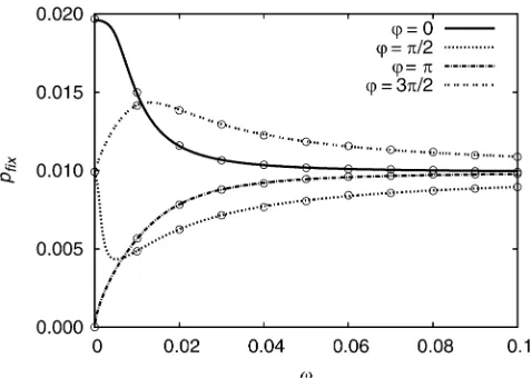
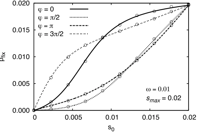
Figure 2 shows how theﬁxation probability changes with

vfor various values ofu. For small and intermediate values ofv, the value ofuhas a strong impact on the result. Ifv increases, thefixation probability converges to the value for a mutation with selective advantages(t) =s0for all values ofu. This behavior is further illustrated in Figure 3, which shows the fixation probability and the initial selection strength in dependence of u for various values of v. In the limit v /0, thefixation probability equals s(0)/(1 +

s(0)) s(0). It therefore follows approximately the curve of s(0) for small values ofv. For large values it converges to s0 for all values of u. In an intermediate regime

s0=10≲v≲10s0, more complex behavior is found: Here, not only the initial value s(0) but also the following time development of the selection strength [i.e., not onlys(0) =

s0(1 + cos(u)), but u itself] becomes important. The ex-trema of pﬁx(u) are attained for smaller values of u than the extrema of s(0). A straightforward calculation shows furthermore that

pfixðueÞ ¼

s0ð1þcosðueÞÞ 1þs0ð1þcosðueÞÞ

; (31)

whereueis the value where the extremum is attained. We thus see that the ﬁxation probability at the extrema ue is the same for cyclic selection and constant selection withs=

s(0) =s0(1 + cos(ue)).

Time to reach an intermediate frequency xc

Analytical theory

In models of the adaptive process, it is often necessary to know the time that it takes for a successful mutation to become established and to reach a certain threshold frequency (e.g., Desai and Fisher 2007; Kopp and Hermisson

2009a). It is well known that the deterministic model of the allele frequency increase yields a poor approximation even for the expected value of this time. The reason is that a mu-tation that has survived the initial phase will on average have grown faster during this phase than predicted by the deterministic model. When the frequency is ﬁnally large enough that stochasticity can be neglected and the path be modeled deterministically, the frequency will thus be larger than if it hadalwaysgrown following the deterministic path. In that phase, it is well described by the deterministic path that is not started from a single individual, but from an (on average) larger “effective initial population size.” The method presented here builds on work by Cohn and Jagers (1994) and Desai and Fisher (2007). It consists of subsum-ing all the stochasticity of the path under this effective initial population size as a single random variable and then mod-eling the path deterministically. The procedure consists of two steps: In a ﬁrst step the distribution of the effective initial population size is estimated via a branching process. In a second step the deterministic approximation of the full birth–death model is used to describe the allele frequency path starting from the effective initial population size.

Let us again consider the phase in which the mutation is rare and in which the dynamics can be described by the time-inhomogeneous branching process (Equation 7). The key to the method is that it is possible to separate stochastic

ﬂuctuations and deterministic growth for this process. Here, deterministic growth coincides with the time-development of the expected number of mutants:

E½nt ¼n0expðrðtÞÞ: (32)

In the following, we restrict to the case n0= 1. Deﬁne now a new random variable:

Figure 2 Comparison between the analytical theory and simulation results for the ﬁxation probability in the case of periodically changing selections(t) =s0(1 + cos(vt+u)),s0= 0.01. Simulations were performed for a population of 100,000 individuals, and every simulation point is the average over 107_runs.

(8)

nt:¼ nt

E½nt¼ntexpð2

rðtÞÞ: (33)

ntdescribes all the stochasticity that has accumulated in the branching process until timet. Crucially, a theorem by Cohn and Jagers (1994) guarantees that fort/N,ntconverges (almost surely) to a positive random variablenthat summa-rizes the entire stochasticity of the process. Since nt =

n exp(r(t)) in the limitt/N, we can interpretenas the random initial population size of an ensemble of determin-istically growing paths that approximate the original process

ntfor larget.

For theﬁxation process, in particular, we are interested in the distribution ofnconditioned on non-extinction. We pro-ceed as follows: From the probability generating function

P(z,t)[P1(z,t) (see Equation 10), we obtain for the prob-abilitypn(t)[pn(1,t) to havenindividuals at timet(proof by induction, see section S3 ofFile S1):

pnðtÞ ¼ 1 n!

dnPðz;tÞ

dzn

z¼0¼

Bn21ðtÞAðtÞ

ðAþ BÞnþ1ðtÞ; n$1: (34)

Conditioning on non-extinction [which requires the bi-ologically meaningful conditionp0(t)6¼1] leads to

Prob½n;tjnot extinct ¼ pnðtÞ 12p0ðtÞ¼

AðtÞ BðtÞ

BðtÞ ðAþBÞðtÞ

:

(35)

By induction, weﬁnd

Ehnk_t not extincti¼ 1 12p0ðtÞ

Ehnk_ti and Ehnk_ti ekrðtÞ;

(36)

i.e., for large times thekth moment grows in the conditioned as well as in the unconditioned process asekr(t)_{. In} particu-lar, we obtain for the expected value

E½ntjnot extinct ¼ 1

12p0ðtÞe

rðtÞ_: ₍₃₇₎

[Since 1=ð12p0ðtÞÞ$1, a comparison with Equation 32 conﬁrms that on average the conditioned path grows faster than the unconditioned path.] The distribution function of

ntjnot extinct is immediately obtained from the distribution function ofntjnot extinct:

Pðnt#n0jnot extinctÞ ¼12

n0

(38)

⇒Pðnt# n0jnot extinctÞ

¼12exp

n0expðrðtÞÞln

: (39)

As limt/NexpðrðtÞÞlnðBðtÞ=ðAþBÞðtÞÞ¼21=ðAþBÞ¼2pfix, we obtain in the limitt/Nthe stationary distribution

Pðn # n0jnot extinctÞ ¼12exp

2pfixn0 : (40)

This effective initial mutant population size may now be used as the starting value for the deterministic solution of the full model. If the birth and death rates are the same for mutants and residents, the latter can be obtained from Equation 4a and is given by a generalized logistic,

xðtÞ ¼ expðbðtÞÞ N0=n21þexpðbðtÞÞ;

(41)

wherex(t) is the mutant frequency and

bðtÞ ¼ ðt

0

sðtÞdt: (42)

We want to calculate the time needed to reach an intermediate frequency xc. Here, intermediate frequency means a frequency at which the dynamics are well described by Equation 41, i.e., not too close to either 0 or 1. Using Equation 41, we can express the random variableTxcdeﬁned

viaxðTxcÞ ¼xcin terms ofn:

Txc¼ (

b21_InxcðN02nÞ

ð12xcÞn

; n,xcN0

0; n $xcN0:

(43)

For the deﬁnition ofTxc to be unique for allxc,the

con-ditions(t).0 (up to single points) is necessary. It is possible that the process grows so quickly that the effective initial mutant population size is already larger than xcN [cf. the exponential tail in the distribution function for the effective initial population size n (Equation 40)]. In this case, we have set Txc ¼0 so that the distribution of Txc will have

a mass on Txc¼0. However, if xc is not too small, this is

very unlikely and the mass will be small. As the determin-istic path (Equation 41) ignores stochastic ﬂuctuations, there is only a single passage time in the deterministic approximation in contrast to the stochastic path in which the frequency xccan be hit several times.Txcas deﬁned in

Equation 43 is best interpreted as the average over all times at which the path crosses the frequencyxcfrom lower to higher values.

By a parameter transformation (n/Txc using Equation

43), the distribution ofTxc is found from Equation 40:

PðTxc #TÞ ¼exp

2 pfixN0

ðð12xcÞ= xcÞexpðbðTÞÞ þ1

: (44)

Equation 44 constitutes the main result of this section.

(9)

two parameters that summarize the time-dependence of the model. For theﬁxation probability, we have seen in Equation 16a that there is a second way to summarize the dynamics in terms of the absolute rate of increase (s+r)(t) and the total rate of birth and death events. This is not possible for the distribution ofTxc, linked to the fact that variable selection

and demographic change are not equivalent in this case. While the selection function s(t) has a strong inﬂuence on the deterministic part of the frequency pathx(t), changes in the total population size (with equal effect on mutants and residents) have no inﬂuence on the latter.

To calculate moments of the distribution, we perform the parameter transformation

Txc/Y:¼

pfixN0

ðð12xcÞ= xcÞexpðbðTxcÞÞ þ1

: (45)

Solving forTxc yields

Txc ¼b

21

ln

xc 12xc

pfixN02Y

Y

; (46)

and we obtain for the moments

hT_xn_ci¼ ðpfixN0xc

0

b21

ln

xc 12xc

pfixN02Y

Y

n

expð2YÞdY:

(47)

For constant selection and thereforeb(t) =stwe obtain for the mean ofTxc:

hTxci ¼

1

s

ln

h pfixN0

i

þgþln

xc 12xc

2 1

pfixN02 1

pfixN0

!2

þ O 1

pfixN0

3

:

(48)

Applications

Constant selection and constant population size: For the distribution of the passage time Txc, we obtain with pfix¼s=ðjþsÞ 2sðNe=NÞ(see Equation 17)

PðTxc#TÞ ¼exp h

2_j s

þs

N

ðð12xcÞ= xcÞexpðsTÞ þ1

exp

h

2 2sNe

ðð12xcÞ= xcÞexpðsTÞþ1 i

:

(49)

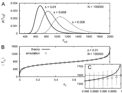
Plots of the probability density for xc= 0.5 and various values ofsare depicted in Figure 4A. With increasing selec-tion strength the distribuselec-tion gets narrower and is shifted to the left.

In the particular situation of constant selection and population size, additional results can be obtained. First,

we note thatTxc can also be interpreted as the age of a

de-rived allele that is currently found at frequency xc in the population. This is a consequence of the time-homogeneity of the model. Second, the distribution of the time to reach

ﬁxation atx = 1 starting from a frequency (12xc) equals the distribution of Txc (see section S3 ofFile S1 for an

ex-planation). In particular, the times needed from 0 to 0.5 and from 0.5 to 1 follow the same distribution. Since both ran-dom variables are independent, we obtain the probability density p~ðtfixÞ of the whole ﬁxation time from the density

p(T1/2) as

~

ptfix

¼

ðt_fix

0

pT1=2

ptfix2T1=2

dT1=2: (50)

An alternative expression for the distribution of tfix has been derived before by Wang and Rannala (2004), using diffusion techniques. We note that our approximation (Equation 50) is simpler than the series expansion in terms of Gegenbauer polynomials, using the eigenvalues of the oblate spheroidal angular function and the intermediate coefficients of the spheroidal harmonics obtained by these authors. As discussed in section S1 ofFile S1, it is neverthe-less highly accurate if selection is not very weak or the pop-ulation size small. The cumulants of the fixation time are just two times the cumulants of the time to reach frequency 0.5. For the meanfixation time, in particular, we obtain

(10)

tfix

¼2

s ln

sN jþs

þg2jþs

sN 2 ðjþsÞ2

ðsNÞ2 þ O

ðjþsÞ3 ðsNÞ3

!! ;

(51)

whereg0.577 is the Euler constant.

For the higher cumulants, approximations of leading order insNcan be obtained by the approximation exp(sT) + 1exp (sT) in the distribution function (Equation 49) and by extending the integral (Equation 47) to inﬁnity. We state the results for the variance, the skewness, and the kurtosis,

k2¼

t2fix

2tfix

2

1

3

p2

s2; (52a)

k3 4zð3Þ

s3 .0; (52b)

k4 2 15

p4

s4.0; (52c)

wherez(z) is the Riemann Zeta function andz(3)1.202 is the Apéry constant. It can be shown that all cumulants of order$2 are to leading order of the form

kj¼cj

1

s j

(53)

with some numerical constantcj.

Sinces.0 is required for the branching approximation, deviations from the exact values must be expected for weak selection. To estimate the precision of our approximation in this case, we compare the result for the meanfixation time to the result obtained from the diffusion approximation. For this purpose we scale time withN(tfix/tfix=tfix/N) and take the diffusion limit (i.e.,s/0,N/Nwitha:=sN/j remaining constant) of Equation 51. We obtain

t_fix¼2_a

lnðaÞ þg21

a2

1

a2þ O

1

a3

: (54)

This is in perfect agreement with the approximation for the

mean ﬁxation time found in Hermisson and Pennings

(2005), using the diffusion approximation. As shown in section S2 ofFile S1, the deviation of our branching process approximation from the exact diffusion result is exponen-tially small ina/2.

Figure 4, B and C, shows the mean time to reach a fre-quency xc in dependence of xc. Signiﬁcant deviations be-tween the theoretical predictions of Equation 49 and simulation results are found only for values of xcthat are extremely close to 1 (or 0). Generally, it holds that the ap-proximation becomes less good forxc≳121/a(orxc≲1/a), as in this regime the deterministic frequency path (Equation 41), which we used in the derivation, is not a good approx-imation to the real frequency path of the mutation (see Ewens 2004, p. 167f).

It is interesting to note that the distribution ofTxc is the

same for beneﬁcial mutations with selective advantagesand deleterious mutations with selective disadvantage 2s (cf. Ewens 2004): For every point of a particular path leading fromn= 1 ton=nc, the sum of the birth and the death rate is the same for both scenarios. This implies that the distri-bution of the run time of this particular path is the same. The chance to be realized differs for each such path by a constant factor ðjþsÞ2nc: _{If we therefore condition on} n=ncbeing reached, the distribution of the time to reach

ncis the same for beneﬁcial and deleterious mutations.

Constant selection and changing population size: Using the expression for pﬁx calculated for a logistically growing population, we immediately get the distribution of the pas-sage time Txc.Figure S5shows a comparison to simulation

results for the second scenario. With Equation 48 we obtain the result for the mean of Txc:

hTxci

1

s

lnhN0_s_ð_r_þ_s_Þþð_b_þ_js_Þððr_sþ_þs_rgÞ

0Þþg0rðrþsÞ i

þgþln

h xc

12xc i

:

(55)

Linearly increasing selection: Putting the expression obtained forpﬁx(Equation 25) into Equation 44, one obtains the distribution of the timeTxc at which a fractionxcof the

population consists of mutant individuals. The distribution can be used to calculate the mean of Txc numerically. A

comparison to simulation results for the distribution and the mean ofTxc in dependence ofs1can be found inFigure S6. From Figure 5, it can be seen that for small values of s0 even a very slight increase of the selection strength over time leads to a drastically smaller mean value ofTxcin

com-parison to an environment with constant selections=s0.

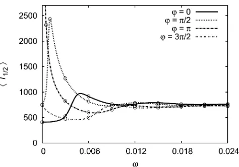
Periodically changing selection: Figure 6 shows the mean time to reach frequency xc = 0.5 for a periodic selection coefﬁcient sðtÞ ¼s0ð1þ cosðvtþuÞÞ. As for the ﬁxation probability, the initial selection strength s(0) is decisive if the environment changes very slowly; uitself gains impor-tance with increasing (but still small)v. If the environment changes fast,hTxcibecomes independent ofuand converges

to its value for constant selection s(t) = s0. Convergence is much faster than for theﬁxation probability.

Simulations

To test our analytical results, we performed individual based computer simulations for which we use a Gillespie

algorithm (Gillespie, 1977). Events happen at rate

ð2jðt;NtÞ1sðt;NtÞÞntðNtntÞ=Nt1bðt;NtÞNt1dðt;NtÞNt; wherej(t, Nt)s(t, Nt),b(t, Nt) andd(t, Nt) are assumed to be constant between events. Once the time of an event is

(11)

andntare updated and the rates are set to their new values (additional update steps between events did not change the results).

For most of the simulation runs, we used theﬁrst passage time of a given frequency xc to determine Txc, i.e., we

neglected ﬂuctuations aroundxc, which for large values of

aand not too small or large values ofxchas no signiﬁcant effect. For the data shown in panel C of Figure 4 and in

Figure S2andFigure S3, where we pushed the boundaries of the theory, we took the average over all passage times, more precisely the average over all times at which the path crossed the frequency xc from lower to higher values (cf. section on the analytical theory).

For all simulation results, the number of runs was chosen sufﬁciently large that the standard error bars vanish in the symbols. All programs were written in C, making use of the Gnu Scientiﬁc Library (Galassiet al., 2009). We used Mathematica (Wolfram Research, Champaign, USA) for all numerical evaluation of integrals.

Discussion

Adaptation is the evolutionary response of a population to an environmental challenge: variation in the environmental conditions leads to altered selection pressures and changing population sizes. In nature, these changes occur on all time scales, from rapid shifts within a single generation to long-term geological trends. It therefore seems natural that models on the genetics of adaptation, too, should account for the ecological dynamics that drive the process. In contrast to this expectation, however, the vast majority of published studies with a genetic focus assume a constant environment (reviewed,e.g., in Orr 2010). They rely on the idea that a fast—almost instantaneous—change in the envi-ronment is followed by a period of envienvi-ronmental stasis. If

this period is long compared to the total time it takes for one or several beneficial mutations to appear and to rise tofi x-ation, ecology and evolution are effectively decoupled. In many cases of ecological interest, however, this separation of time scales is not appropriate. In this case, the parameters of the evolutionary model (such as selection coefficients or population sizes) are turned into time-dependent variables, which must be determined from an underlying ecological model.

In a series of recent publications by several authors, the impact of the ecological dynamics on the genetics of adaptation has been studied for the so-called moving optimum model (Bello and Waxman 2006; Collins et al.

2007; Kopp and Hermisson 2007, 2009a,b). The consensus, at least for this model, is that the adaptive process is strongly affected by the dynamics of the selective environment. In this article, we present a more detailed treatment of the most basic aspect of the genetics of adaptation: thefixation process of a single beneficial mutation in a variable environ-ment. All relevant parameters of the process, i.e., selection coefficient, population size, and the variance in offspring number (or, equivalently, the birth and death rates of wild types and mutants) may depend explicitly on time. An ex-ample of how this can result from an explicit ecological model is given in theAppendix, where we discuss thefi xa-tion probability of a“rescue mutation”in a population that is otherwise doomed to extinction. Again, the results are strongly influenced by the ecological dynamics, leading to qualitative differences relative to previous studies that as-sume constant selection (Orr and Unckless 2008).

Even if the external environment is constant, individual alleles in a population can experience variable selection pressures if multiple selected alleles segregate in the popu-lation and if these alleles interfere due to either epistasis or linkage (cf. Hartﬁeld and Otto 2011). Examples include the evolution of compensatory mutations or classical problems of clonal interference, where the beneﬁcial mutation rate is

Figure 5 Mean time to reach frequencyxc= 0.5 in dependence ofs0, where a scenario with constant selection and a scenario with linearly increasing selection (s1= 1/80,000) are compared. The meanﬁxation time is signiﬁcantly smaller in the case of linearly increasing selection than in the case of constant selection. Each simulation point is the average over 1000 runs.

(12)

high relative to the recombination rate. Another potential application is adaptive gene ﬂow across a genetic barrier, where adaptations need to be purged from linked deleteri-ous alleles by recombination.

Using branching process techniques, we obtain analytical approximations for theﬁxation probability and the distribu-tion of the time for the mutant to reach a given frequencyxc in the population.

Fixation probability

The derivation of fixation probabilities of rare beneficial mutations from a supercritical branching process is a stan-dard approach in population genetics. In particular, results have previously been obtained for the most important modes of demographic changes (e.g., Otto and Whitlock 1997; Pollak 2000). A look into the mathematical literature reveals, however, that a general formalism with arbitrary time-dependent birth and death rates has been available since the work of Kendall (1948). In contrast to most of the previous studies in population genetics, which use a branching process in discrete time (following Haldane 1927), this approach is based on a continuous-time frame-work, which simplifies some technical aspects. Our adapta-tion of this formalism to the genetic context leads to a compact, yet general formula for the fixation probability

pﬁx(Equations 16a and 16b) that covers previous results as special cases. In section S2 of File S1, we show how an analogous result can also be obtained using the diffusion approach.

It turns out that the ecological dynamics affect pfix through two independent variables. In two alternative formulations of the result, these can be either the time-dependent birth and death rates of rare mutants (Equation 16a) or the selection coefficients(t) and the variance effec-tive population size Ne(t) (Equation 16b). Our applications to various scenarios show that relative to the case with con-stant selections0, consistent changes in the selection coeffi -cientDsper generation of the order ofDs$s2

0have a strong effect on pﬁx.This is to be expected since, for constant se-lection, the fate of a new mutation (ﬁxation or loss) is de-cided once the mutant allele reaches a frequency on the order of (Ns0)21. According to Equation 48, this will take, on average, in the order ofs21

0 generations. The observation is of practical importance since it shows that predictions about ﬁxation probabilities cannot be based on short-term

fitness assays. Unmeasurably small fitness changes across generations may have a large effect. The limitations of the branching approach are the usual ones: The fate of the mu-tation must be decided while the mutant frequency is small and the independence assumption of the branching process applies. Deviations from the simulation results are found in the case of mutations that are almost neutral on average, with fixation probabilitiespfix≲10/N(cf.File S1).

Time Txcto reach frequency xc

The usual method in population genetics to derive fixation times or (more generally) first-passage times for mutant alleles to reach certain frequencies is diffusion theory. Since this proves difficult for the time-inhomogeneous case, we again turn to a branching process approach. We can use the fact that (almost) all stochasticity of a mutant trajectoryx(t) is due to its early phase while the mutant number is still small. We can therefore (approximately) describe this sto-chasticity in the branching framework and combine it with the deterministic growth of the full process. For constant selection and population sizes, this idea has previously been used by Desai and Fisher (2007) in the context of a model for clonal evolution.

For the general case, the crucial step of the method has again been anticipated in the mathematical literature (Cohn and Jagers 1994). There, it has been shown that a clean separation exists for the random variablentof an inhomoge-neous supercritical branching process into a growth function that describes the asymptotic growth and a time-constant random variablenthat describes the stochasticfluctuations in the large-time limit. We can interpret n as the effective initial size of the mutant population. It turns out that the distribution function of n, P(n # n0|not extinct) = 1 2 exp(2pfixn0) (Equation 40), is pleasingly simple even in a variable environment. In particular, the impact of the ecological dynamics is conveniently summarized in thefi x-ation probability pfix. When this initial size is combined with the deterministic growth of the full model, an approx-imation for the distribution function forTxc is obtained by

a simple transformation of the probability density (Equa-tion 44).

(13)

frequency ofxc= 1 is not an absorbing state and may never be reached in the face of back mutation, migration, or on-going adaptation. For many practical applications, other thresholds (such as 5%, 50%, or 95%) are therefore more relevant and have previously been used. For example, Desai and Fisher (2007) use a threshold ofxc= 1/(Ns) to charac-terize their establishment time test. Kopp and Hermisson (2007, 2009a) usexc= 0.5 as the critical value where the mutant comes to dominate the population in an analysis of the order and step sizes of adaptive substitutions.

Although we have formulated our results for haploids, they also apply to diploids as long as the mutant is not fully recessive (i.e., hs must be sufﬁciently large on average). Only the selection coefﬁcients (or birth and death rates) of heterozygotes enter into the stochastic part of the model described by the branching process. In contrast, the deter-ministic frequency path used in the derivation ofTxcdepends

on theﬁtness values of both heterozygous and homozygous mutants. In the purely recessive case, the dynamics of rare mutants can no longer be described by a supercritical branching process. Diffusion methods (for constant selec-tion) show that also the scaling of the ﬁxation time with the selection parameters is altered in this case (Ewing

et al.2011).

To summarize, our results show that inhomogeneous branching processes provide a powerful framework to de-scribe the ﬁxation process under a wide range of ecological scenarios and genetic conditions. We therefore hope that the methods and results can provide a step to combine ecological and genetic modeling traditions to study the genetics of adaptation under realistic ecological conditions.

Note: After acceptance of this article we became aware of a recent preprint by Waxman on thefixation process under variable selection and demography [see D. Waxman (pp. 907–913) in this issue]. Both articles are complementary: While our approach focuses on analytical approximations for thefixation process of a definitely beneficial mutant, Wax-man (2011) presents numerical methods to derive fixation probabilities for alleles with arbitrary selection coefficients.

Acknowledgments

We thank Nick Barton, Ulf Dieckmann, Peter Pfaffelhuber, and Matthew Hartﬁeld for helpful discussions and Lindi Wahl and two anonymous referees for many useful com-ments. This work was made possible with ﬁnancial support from the Vienna Science and Technology Fund and from the Deutsche Forschungsgemeinschaft, Research Unit 1078,

Natural selection in structured populations.

Literature Cited

Allen, L. J. S., 2011 An Introduction to Stochastic Processes with

Applications to Biology, Ed. 2. Pearson Education, Upper Saddle River, NJ.

Barton, N. H., 1995 Linkage and the limits to natural selection.

Genetics 140: 821–841.

Bello, Y., and D. Waxman, 2006 Near-periodic substitutions and

the genetic variance induced by environmental change. J. Theor.

Biol. 239: 152–160.

Chia, A. B., 1968 Random mating in a population of cyclic size.

J. Appl. Probab. 5: 21–30.

Cohn, H., and P. Jagers, 1994 General branching processes in

varying environment. Ann. Appl. Probab. 4(1): 184–193.

Collins, S. J., J. de Meaux,, and C. Acquisti, 2007 Adaptive walks

toward a moving optimum. Genetics 176: 1089–1099.

Desai, M. M., and D. S. Fisher, 2007 Beneﬁcial mutation-selection

balance and the effect of linkage on positive selection. Genetics

176: 1759–1798.

Ewens, W. J., 1967 The probability of survival of a new mutant in

a_ﬂuctuating environment. Heredity 22: 438_–443.

Ewens, W. J., 2004 Mathematical Population Genetics, Ed. 2.

Springer-Verlag, New York.

Ewing, G., J. Hermisson, P. Pfaffelhuber, and J. Rudolf,

2011 Selective sweeps for recessive alleles and for other

modes of dominance. J. Math. Biol. (in press).

Fisher, R. A., 1922 On the dominance ratio. Proc. R. Soc. Edinb.

42: 321–341.

Fisher, R. A., 1930 The distributions of gene ratios for rare

muta-tions. Proc. R. Soc. Edinb. 50: 204–219.

Galassi, M., J. Davies, J. Theiler, B. Gough, G. Jungman, et al.,

2009 GNU Scientiﬁc Library Reference Manual,Ed. 3. Network Theory Ltd., Bristol, UK.

Gillespie, D. T., 1977 Exact stochastic simulation of coupled

chemical reactions. J. Phys. Chem. 81(25): 2340–2361.

Haccou, P., P. Jagers, and V. A. Vatutin, 2005 Branching Processes.

Variation,Growth and Extinction of Populations. Cambridge Uni-versity Press, Cambridge, UK.

Haldane, J. B. S., 1927 A mathematical theory of natural and

artiﬁcial selection. V. Selection and mutation. Proc. Camb.

Philos. Soc. 23: 838–844.

Hartﬁeld, M., and S. P. Otto, 2011 Recombination and

hitchhik-ing of deleterious alleles. Evolution (in press).

Hermisson, J., and P. S. Pennings, 2005 Soft sweeps: molecular

population genetics of adaptation from standing genetic

varia-tion. Genetics 169: 2335_–2352.

Huillet, T., 2011 On the Karlin-Kimura approaches to the

Wright-Fisher diffusion with _ﬂuctuating selection. J. Stat. Mech. 2_:

P02016.

Jensen, L., 1973 Random selective advantages of genes and their

probabilities ofﬁxation. Genet. Res. 21(3): 215–219.

Karlin, S., and B. Levikson, 1974 Temporalﬂuctuations in

selec-tion intensities: case of small populaselec-tion size. Theor. Popul. Biol.

6: 383–412.

Kendall, D. G., 1948 On the generalized “birth-and-death”

pro-cess. Ann. Math. Stat. 19(1): 1–15.

Kimura, M., 1962 On the probability ofﬁxation of mutant genes

in a population. Genetics 47: 713–719.

Kimura, M., and T. Ohta, 1969 The average number of

genera-tions untilﬁxation of a mutant gene in aﬁnite population.

Ge-netics 61: 763–771.

Kimura, M., and T. Ohta, 1974 Probability of geneﬁxation in an

expanding ﬁnite population. Proc. Natl. Acad. Sci. USA 71:

3377–3379.

Kopp, M., and J. Hermisson, 2007 Adaptation of a quantitative

trait to a moving optimum. Genetics 176: 715–719.

Kopp, M., and J. Hermisson, 2009a The genetic basis of

pheno-typic adaptation I:ﬁxation of beneﬁcial mutations in the moving

optimum model. Genetics 182: 233–249.

Kopp, M., and J. Hermisson, 2009b The genetic basis of

pheno-typic adaptation II:_ﬁxation of bene_ﬁcial mutations in the

(14)

Moran, P. A. P., 1958a The effect of selection in a haploid genetic

population. Math. Proc. Camb. Philos. Soc. 54: 463–467.

Moran, P. A. P., 1958b Random processes in genetics. Proc.

Camb. Philos. Soc. 54: 60–71.

Novozhilov, A. S., G. P. Karev, and E. V. Koonin, 2006 Biological

applications of the theory of birth-and-death processes. Brief.

Bioinform. 7(1): 70_–85.

Ohta, T., and K.-I. Kojima, 1968 Survival probabilities of new

inversions in large populations. Biometrics 24(3): 501_–516.

Orr, H. A., 2010 The population genetics of bene_ﬁcial mutations.

Philos. Trans. R. Soc. B 365: 1195_–1201.

Orr, H. A., and R. L. Unckless, 2008 Population extinction and the

genetics of adaptation. Am. Nat. 172(2): 160_–169.

Otto, S. P., and M. C. Whitlock, 1997 The probability of_ﬁxation in

populations of changing size. Genetics 146: 723_–733.

Parsons, T. L., and C. Quince, 2007a Fixation in haploid

popula-tions exhibiting density dependence I: the non-neutral case.

Theor. Popul. Biol. 72: 121–135.

Parsons, T. L., and C. Quince, 2007b Fixation in haploid

popula-tions exhibiting density dependence II: the quasi-neutral case.

Theor. Popul. Biol. 72: 468–479.

Patwa, Z., and L. M. Wahl, 2008 Theﬁxation probability of

ben-eﬁcial mutations. J. R. Soc. Interface 5: 1279–1289.

Pollak, E., 1966 Some effects ofﬂuctuating offspring distributions

on the survival of genes. Biometrika 53(3/4): 391–396.

Pollak, E., 2000 Fixation probabilities when the population size

undergoes cyclicﬂuctuations. Theor. Popul. Biol. 57: 51–58.

Takahasi, K. R., and F. Tajima, 2005 Evolution of coadaptation in

a two-locus epistatic system. Evolution 59(11): 2324–2332.

Takahata, N., K. Ishii, and H. Masuda, 1975 Effect of temporal

ﬂuctuation of selection coefﬁcient on gene frequency in a

popu-lation. Proc. Natl. Acad. Sci. USA 72: 4541–4545.

Wahl, L. M., and P. J. Gerrish, 2001 The probability that beneﬁ

-cial mutations are lost in populations with periodic bottlenecks.

Evolution 55: 2606_–2610.

Wang, Y., and B. Rannala, 2004 A novel solution for the

time-dependent probability of gene ﬁxation or loss under natural

selection. Genetics 168: 1081_–1084.

Waxman, D., 2011 A uniﬁed treatment of the probability ofﬁ

xa-tion when populaxa-tion size and the strength of selecxa-tion change

over time. Genetics 188: 907_–913.

Whitlock, M. C., 2003 Fixation probability and time in subdivided

populations. Genetics 164: 767_–779.

Whitlock, M. C., and R. Gomulkiewicz, 2005 Probability of_ﬁxation

in a heterogeneous environment. Genetics 171: 1407_–1417.

Communicating editor: L. M. Wahl

Appendix

Fixation in General Ecological Models

In this Appendix, we describe how the branching process approach can be applied to a general ecological scenario where the genetic composition of the population and the population dynamics are mutually dependent. Assume that at time t a population consists of wt wild-type “residents” and nt mutants. Both types reproduce and die at different per capita rates, which may depend on the number of resi-dents and mutants, wtand nt, and on external factors that are independent of the population, but also may change over time. A general framework, which takes the full dynam-ics with all kinds of interactions between types into account, is given by the following scheme of transition rates:

nt/ntþ1: nt h

bð₁mÞðtÞ þbð₂mÞðtÞntþbð₃mÞðtÞwtþ. . . i

;

nt/nt21: nt h

dð₁mÞðtÞ þdð₂mÞðtÞntþdð₃mÞðtÞwtþ. . . i

;

wt/wtþ1: wt h

bð₁wÞðtÞ þbð₂wÞðtÞwtþbð₃wÞðtÞntþ. . . i

;

wt/wt21: wt h

dð₁wÞðtÞ þdð₂wÞðtÞwtþdð3wÞðtÞntþ. . . i

:

(A1)

Higher-order interaction terms with transition rates pro-portional to any polynomial in nt andwt can be added as needed. The model corresponds to a general two-dimensional birth–death process with time-dependent coefﬁcients. For such a model, the corresponding deterministic evolution of

nt and wt is generically given by a system of two coupled

differential equations. In most cases, it is impossible to solve this system analytically. Since the determinstic frequency path of the mutant is needed for the theory developed to calculate

Txc, derivations forTxc must resort to numerical solutions to

apply the methods outlined in the main text. In contrast, an analytical approximation for the ﬁxation probability (and thus also the distribution of the effective initial population sizen,cf. Equation 40) is often still possible.

In the branching limit of rare mutant individuals, all interactions of either residents or mutants with (other) mutant individuals can be neglected. Mathematically, this corresponds to the approximation nt 0 in the birth and death rates of the residents and negligence of all terms of order O(nt) .1 in the transition rates of the mutants. As a consequence, the evolution of the residents is decoupled from the mutants. In the deterministic limit, the time de-velopment of the resident population size w(t) N(t) is then given by an ordinary differential equation that can frequently be solved explicitly. We can then describe the dynamics of rare mutants by a one-dimensional branching process. Inserting the deterministic solution forw(t) into all mutant transition rates of linear order in the mutant number

(15)

methods and has the advantage that it can be applied to neutral and deleterious mutation, too (Parsons and Quince 2007a,b), which is beyond the reach of the branching model. However, it cannot easily be extended to the time-inhomogeneous case that is our focus here.

Rescue mutation

Consider, as an example, the following scenario: A population is subject to a new and severe selection pressure (e.g., new insecticide, drug, parasite, competitor, . . .). As a consequence, the population size decreases, and selection will drive the population to extinction unless a rescue mu-tation can be established that confers immunity to its car-riers. A similar scenario has been discussed by Orr and Unckless (2008).

A plausible ecological model for this situation could be as follows: The original resident population evolves under logistic population dynamics with growth parameter r and time-dependent carrying capacity K(t). Due to the environmental challenge, the carrying capacity decreases exponentially like

K(t) =K0exp(2at). At the individual level, the model can be described in the scheme of Equation A1,

bð₁wÞðtÞ ¼r; d₂ðwÞðtÞ ¼dð₃wÞðtÞ ¼r 1

KðtÞ; (A2)

with all other coefﬁcientsbðiwÞðtÞanddð wÞ

i ðtÞequal to zero. As long as the number of beneﬁcial mutants is small, the wild-type population size changes according to

wðtÞ ¼ K0ðaþrÞ

a expð2rtÞ þr expðatÞ: (A3)

Assume now that a beneﬁcial mutation—if it survives stochastic loss—restores population size to its original car-rying capacityK0=K(0);i.e.,

bð₁mÞðtÞ ¼r; d₂ðmÞðtÞ ¼dð₃mÞðtÞ ¼r1

K0 (A4)

(and again all other coefﬁcients are equal to zero). The

ﬁxation probability of a single mutation arisingttime units after the decline in the carrying capacity started is then given by

pfixðtÞ ¼2

1þ

ðN

0 r

1þwðtþtÞ

K0

exp

2ðt 0 r

12wðtþxÞ

K0

dx

dt

21

:

(A5)

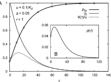
In Figure A1 thefixation probability of a single mutation and the ratiog0(t) =w(t)/K0=N(t)/K0are shown in de-pendence of t. Note that the fixation probability increases with t: While the mutant does not have a higher intrinsic growth rate than the resident (in a variant of the model, it could even be lower), it thrives due to relaxed competition as the resident population declines. However, for a given mutation probability per time unit ufrom resident to mu-tant, the new total rate of beneficial mutations is propor-tional to the resident population size and thus decreases with t. The rate at which new successful mutations arise is given byufix(t) =uw(t)pfix(t), which reaches a maximum at some intermediate timet* (see Figure A1). The probability that a successful mutation arises before timeTis

Pðt#TÞ ¼12exp

2

ðT

0

u_fixðtÞdt

: (A6)

The probability that a successful mutation arises at all,

i.e., that the population is rescued from extinction, is there-fore given by

Prescue¼12exp

2

ð_N

0

ufixðtÞdt

: (A7)

This probability is equal to 1 if and only if the integral

Ð_N

0ufixðtÞdt diverges, i.e., if the rate ufix(t) declines suffi -ciently slowly. Otherwise the probability that the population is saved from extinction by a rescue mutation is,1, as was also found by Orr and Unckless (2008). For the parameter values used in Figure A1 the survival probability of the popu-lation is calculated to bePrescue0.39. Given the population is rescued, the probability that the rescuing mutation arises in the infinitesimal time interval [t,t+dt] is given byp(t)dt with

pðtÞ ¼ufixðtÞexp

2Ðt0ufixðt^Þdt^

Prescue : (A8)

(16)

For not too large mutation probabilities (u≲0.5/K0for the chosen parameter values), this function has a maximum at an intermediate value oft=t**, as also shown in Figure A1. This result is in contrast to Orr and Unckless (2008), whoﬁnd a monotonic decrease in the (conditioned) proba-bility that a successful mutation arises in a given generation independently of the mutation rate. This is due to the as-sumption in Orr and Unckless (2008) that the selection

(17)

GENETICS

Supporting Information

http://www.genetics.org/content/suppl/2011/06/06/genetics.110.124297.DC1

On the Fixation Process of a Beneﬁcial Mutation

in a Variable Environment

Hildegard Uecker and Joachim Hermisson

(18)

H. Uecker and J. Hermisson

-0.2 -0.15 -0.1 -0.05 0 0.05 0.1 0.15 0.2

0 5 10 15 20 25

p_fixN

s₀ = 0

N = 10000

Figure S1: Relative deviation between analytical and simulation results for an allele with selective advantage

s(t) =s₁t. The empty dots are obtained from branching process approximation, the small ﬁlled dots from the

corrected version Eq. (S1). One sees that the corrected version provides a much better approximation for small

values of p_{f ix}N; for large values of p_{f ix}N, the results coincide. Simulations were performed for a population of

N = 10 000 individuals, and each simulation point is the average over 5·107_runs.

S1

Accuracy of the approximation

Weak selection. As pointed out in the main text, deviations from the exact solution are expected for weak selection.

For an allele with constant selective advantage andN=const., a comparison to the exact solution is immediately

possible (see main text).

As a further example, we consider the ﬁxation probability of an allele with s(t) = s₁t and examine the relative

error between theoretical prediction and simulation results in dependence ofp_{f ix}N (see Figure S1). A relative error

of less than 2% is found forp_{f ix}N <10. The results for small values ofp_{f ix}N can be improved if we correct the

branching approximation by a factor 1/(1−exp (−p_{f ix}N)):

p_{f ix}∗ = pf ix

1−exp (−p_{f ix}N). (S1)

This heuristic approximation is inspired by Eq. (18). The relative deviation from the simulation results is added to Figure S1. It is seen that the approximation is considerably improved.

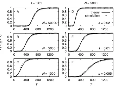
In Figure S2, we compare the distribution function ofT₁_/₂to simulation results for various values ofsandN where

s andN are constant. While agreement is excellent for high values ofα, deviations increase for decreasing values

ofα. A maximum absolute deviation of≥0.05 between theory and simulations is found forα=Ns 10.