Genotyping Polyploids from Messy Sequencing Data

(1)

HIGHLIGHTED ARTICLE

| INVESTIGATION

Genotyping Polyploids from Messy Sequencing Data

David Gerard,*,1_{Luis Felipe Ventorim Ferrão,}†_{Antonio Augusto Franco Garcia,}‡ and Matthew Stephens§,_**

*Department of Mathematics and Statistics, American University, Washington, DC 20016,†Horticultural Sciences Department, University of Florida, Gainesville, Florida 32611,‡Department of Genetics, Luiz de Queiroz College of Agriculture, University of São Paulo, Piracicaba, 13418-900, Brazil, and§Department of Human Genetics and **Department of Statistics, University of Chicago, Illinois 60637 ORCID IDs: 0000-0001-9450-5023 (D.G.); 0000-0002-9655-4838 (L.F.V.F.); 0000-0003-0634-3277 (A.A.G.); 0000-0001-5397-9257 (M.S.)

ABSTRACT Detecting and quantifying the differences in individual genomes (i.e., genotyping), plays a fundamental role in most modern bioinformatics pipelines. Many scientists now use reduced representation next-generation sequencing (NGS) approaches for genotyping. Genotyping diploid individuals using NGS is a well-studied ﬁeld, and similar methods for polyploid individuals are just emerging. However, there are many aspects of NGS data, particularly in polyploids, that remain unexplored by most methods. Our contributions in this paper are fourfold: (i) We draw attention to, and then model, common aspects of NGS data: sequencing error, allelic bias, overdispersion, and outlying observations. (ii) Many datasets feature related individuals, and so we use the structure of Mendelian segregation to build an empirical Bayes approach for genotyping polyploid individuals. (iii) We develop novel models to account for preferential pairing of chromosomes, and harness these for genotyping. (iv) We derive oracle genotyping error rates that may be used for read depth suggestions. We assess the accuracy of our method in simulations, and apply it to a dataset of hexaploid sweet potato (Ipomoea batatas). An R package implementing our method is available athttps://cran.r-project.org/package=updog.

KEYWORDSGBS; RAD-Seq; sequencing; hierarchical modeling; read-mapping bias

N

EW high-throughput genotyping methods (e.g., Davey et al.2011) allow scientists to pursue important genetic, ecological, and evolutionary questions for any organism, even those for which existing genomic resources are scarce (Chenet al.2014). These methods combine high-throughput sequencing with preparation of a reduced representation li-brary, to sequence a small subset of the entire genome across many individuals. This strategy allows both genome-wide single nucleotide polymorphism (SNP) discovery and SNP genotyping at a reduced cost compared to whole-genome sequencing (Chenet al.2014; Kimet al.2016). Speciﬁc ex-amples of these methods include“restriction site-associated DNA sequencing”(RAD-seq) (Bairdet al.2008) and“ geno-typing-by-sequencing”(GBS) (Elshireet al. 2011). Both of

these approaches have been widely used in recent biological research, including in population-level analyses (Byrneet al. 2013; Schillinget al.2014), quantitative trait loci mapping (Spindel et al. 2013), genomic prediction (Spindel et al. 2015), expression quantitative trait loci discovery (Liuet al. 2017), and genetic mapping studies (Shirasawaet al.2017). Statistical methods for SNP detection and genotype calling play a crucial role in these new genotyping technologies. And, indeed, considerable research has been performed to develop such methods (Nielsenet al.2011). Much of this research has focused on methods for diploid organisms—those with two copies of their genomes. Here, we focus on developing meth-ods for polyploid organisms—speciﬁcally for autopolyploids, which are organisms with more than two copies of their ge-nome of the same type and origin, and present polysomic inheritance (Garciaet al.2013). Autopolyploidy is a common feature in plants, including many important crops (e.g., sug-arcane, potato, several forage crops, and some ornamental

ﬂowers). More generally, polyploidy plays a key role in plant evolution (Otto and Whitton 2000; Soltis et al.2014) and plant biodiversity (Soltis and Soltis 2000), and understand-ing polyploidy is important when performunderstand-ing genomic

Manuscript received August 3, 2018; accepted for publication August 21, 2018; published Early Online September 5, 2018.

Supplemental material available at Figshare: https://doi.org/10.25386/genetics. 7019456.

1_{Corresponding author: Department of Mathematics and Statistics, American}

(2)

selection and predicting important agronomic traits (Udall and Wendel 2006). Consequently, there is strong interest in genotyping polyploid individuals, and, indeed, the last de-cade has seen considerable research into genotyping in both non-NGS (next-generation sequencing) data (Voorripset al. 2011; Serang et al.2012; Garciaet al.2013; Bargary et al. 2014; Mollinari and Serang 2015; Schmitz Carleyet al.2017) and NGS data (McKennaet al.2010; Li 2011; Garrison and Marth 2012; Blischak et al.2016, 2018; Maruki and Lynch 2017; Clarket al.2018).

Here, we will demonstrate that current analysis methods, though carefully thought out, can be improved in several ways. Current methods fail to account for the fact that NGS data are inherently messy. Generally, samples are genotyped at low coverage to reduce cost (Glaubitzet al.2014; Blischaket al. 2018), increasing variability. Errors in sequencing from the NGS platforms abound (Li et al.2011) (Modeling sequencing error). These are two well-known issues in NGS data. In this paper, we will further show that NGS data also face issues of systematic biases (e.g., resulting from the read-mapping step) (Modeling allelic bias), added variability beyond the effects of low-coverage (Modeling overdispersion), and the frequent oc-currence of outlying observations (Modeling outliers). Ourﬁrst contribution in this paper is highlighting these issues on real data and then developing a method to account for them.

Our second contribution is to consider information from Mendelian segregation in NGS genotyping methods. Many experimental designs in plant breeding are derived from progeny test data (Li et al. 2014; Tennessen et al. 2014; McCallumet al.2016; Shirasawaet al.2017). Such progenies often result from a biparental cross, including half and full-sib families, or from selfing. This naturally introduces a hierar-chy that can be exploited to help genotype individuals with low coverage. Here, we implement this idea in the case of autopolyploids with polysomic inheritance and bivalent non-preferential pairing. Hierarchical modeling is a powerful sta-tistical approach, and others have used its power in polyploid NGS SNP genotyping, not with Mendelian segregation, but in assuming Hardy-Weinberg equilibrium (HWE), or small de-viations from HWE (Li 2011; Garrison and Marth 2012; Maruki and Lynch 2017; Blischaket al.2018). Using Mende-lian segregation for SNP genotyping has been used in non-NGS data (Seranget al.2012; Schmitz Carleyet al.2017), and in diploid NGS data (Zhou and Whittemore 2012), but, to our knowledge, we are thefirst to implement this for poly-ploid NGS data—though others have used deviations from Mendelian segregation as a way to filter SNPs (Chenet al. 2014,e.g.) or for the related problem of haplotype assembly (Motazediet al.2018).

Though wielding Mendelian segregation in species that exhibit bivalent nonpreferential pairing can be a powerful approach, in some species this assumption can be inaccurate. Chromosomal hom(oe)ologues might exhibit partial or complete degrees of preferential pairing (Voorrips and Maliepaard 2012). Our next contribution is developing a model and inference procedures to account for arbitrary

levels of preferential pairing in bivalent pairing species. In particular, this approach allows us to estimate if a species contains completely homologous chromosomes (autopolyploids), completely homeologous chromosomes (allopolyploids), or some intermediate level of chromosomal pairing (Stiftet al. 2008) (“segmental allopolyploids,”Stebbins 1947). We har-ness these estimates of preferential pairing to genotype (auto/allo)polyploids.

Ourfinal contribution concerns the question raised by the development of our new model:“How many reads are needed to adequately genotype an individual?”This is a complicated by the fact that read depth calculations depend on many factors: the level of allelic bias, the sequencing error rate, the overdispersion, the distribution of genotypes in the sam-ple, as well as the requirements of the intended downstream analyses. This last consideration is especially difficult to con-sider when coming up with general guidelines. For example, in association studies, merely a strong correlation with the true genotype is necessary (Pritchard and Przeworski 2001), and a smaller read depth might be adequate, whereas for mapping studies, a few errors can inflate genetic maps (Hackett and Broadfoot 2003), and so a larger read depth might be needed to improve accuracy. Rather than try to account for all of these contingencies, we took the approach of developing functions that a researcher may use to obtain lower bounds on the read depths required based on (i) the specifics of their data, and (ii) the needs of their study. This is in alignment with the strategy in elementary statistics of not providing general guidelines for the sample size of at-test, but rather provide functions to determine sample size based on the variance, effect size, power, and significance level.

Our paper is organized as follows. We develop our method using a real dataset (Shirasawaet al.2017) as motivation in Methods. During this development, we highlight several issues and solutions to genotyping NGS data, including overdispersion, allelic bias, and outlying observations. We then evaluate the performance of our method using Monte Carlo simulations (Simulation comparisons to other methods throughSimulations on preferential pairing) and demonstrate its superior genotyping accuracy to competing methods in the presence of overdispersion and allelic bias. We then use our method on a real dataset of hexaploid sweet potato (Ipomoea batatas) in Sweet potato. Oracle genotyping rates are ex-plored in Using oracle results for sampling depth guidelines andSampling depth suggestions. Weﬁnish with a discussion and future directions (Discussion).

Methods

(3)

To illustrate key features of our model, we give exam-ples from a dataset on autohexaploid sweet potato samexam-ples (I. batatas) (2n = 6x = 90) from a genetic mapping study by Shirasawaet al.(2017). These data consist of an S1 pop-ulation of 142 individuals, genotyped using double-digest RAD-seq technology (Peterson et al. 2012). Here and throughout,“S1”refers to a population of individuals produced from the self-pollination of a single parent. We used the data resulting from the SNP selection andfiltering procedures de-scribed in Shirasawaet al.(2017). These procedures included mapping reads onto a reference genome of the relatedI. trifida to identify putative SNPs, and then selecting high-confidence biallelic SNPs with coverage of#10 reads for each sample and with ,25% of samples missing, yielding a total of 94,361 SNPs. Further details of the biological materials, assays, and datafiltering may be found in Shirasawaet al.(2017).

For each SNP, we use A and a to denote the two alleles, with A being the reference allele (deﬁned by the allele on the reference genome of the relatedI. triﬁda). For each individ-ual the data at each SNP are summarized as the number of reads carrying the A allele and the number carrying the a allele. For aK-ploid individual there areKþ1 possible geno-types, corresponding to 0;1;. . .;Kcopies of the A allele. We usepi2 f0=K;1=K;. . .;K=Kgto denote the A allele dosage of individuali(soKpi is the number of copies of allele A). Genotyping an individual corresponds to estimatingpi:

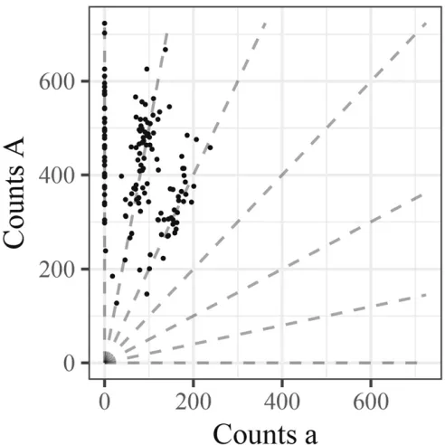
Figure 1 illustrates the basic genotyping problem using data from a single well-behaved SNP. In this“genotype plot” each point is an individual, with thexandyaxes showing the number of a and A reads, respectively. The lines in the plot indicate the expected values for possible genotype pi2 f0=K;1=K;. . .;K=Kg;and are deﬁned by

A

Aþa¼pi; (1)

whereAis the count of A reads andais the count of a reads. Genotyping each sample effectively corresponds to determin-ing which line gave rise to the sample’s data. In this case, the

determination is fairly clear because the SNP is particularly well-behaved and most samples have good coverage. Later, we will see examples where the determination is harder. Naive model

A simple and natural model is that the reads at a given SNP are independent Bernoulli random variables:

xijjpi BernoulliðpiÞ; (2)

wherexijis 1 if readjfrom individualiis an A allele, and is 0 if the read is an a allele. The total counts of allele A in individual ithen follows a binomial distribution

yi¼

Xni

j¼1

xij Binomialðni;piÞ: (3)

If the individuals are siblings, then, by the rules of Mendelian segregation, the pi values have distribution (Serang et al. 2012):

Xk

i¼0

HG

i;K 2 ℓ1;K

HG

k2i;K

2 ℓ2;K

(4)

where~pjis the A allele dosage of parentj, and HGða;bjc;dÞis the hypergeometric probability mass function:

HGða;bjc;dÞ ¼

c a

d2c b2a

d b

: (5)

Equation 4 results from a convolution of two hypergeometric random variables. The distribution (4) effectively provides a prior distribution forpi;given the parental genotypes. If the parental genotypes are known, then this prior is easily com-bined with the likelihood (3) to perform Bayesian inference for pi: If the parental genotypes are not known, then it is straightforward to estimate the parental genotypes by maxi-mum likelihood, marginalizing out thepi;yielding an empir-ical Bayes procedure.

Modeling sequencing error

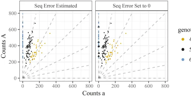
Though model (2) is a reasonable starting point, it does not account for sequencing error. Even if sequencing errors rates are low (e.g., 0.5–1% (Liet al.2011)), it is crucial to model them because a single error can otherwise dramatically im-pact genotype calls. In particular, if an individual truly has all reference allelesðpi¼1Þthen (in the model without errors) a single nonreference allele observed in error would yield a likelihood (and hence posterior probability) of 0 for the true genotype. Biologically, this means that a homozygous indi-vidual can be erroneously classiﬁed as heterozygous, which may impact downstream analyses (Bourkeet al.2018). We demonstrate this in Figure 2 where, in the right panel, weﬁt the model described inNaive modelto a single SNP. We la-beled six points on Figure 2 with triangles that we think Table 1 Summary of notation

Term Deﬁnition

K Ploidy of the species.

xij jth read forith individual.

Equal to 1 if a read is an A and 0 if a read is an a.

yi ¼Pjxij. The number of A reads in individuali. ni Number of reads in individuali.

pi Allele-dosage for individuali,pi2 f0=K;1=K;. . .;K=Kg. u_i Probability sampleiis a nonoutlier.

~

yℓ Number of A reads in theℓth parent. ~

nℓ Number of reads in theℓth parent. ~

pℓ Allele-dosage for theℓth parent. ~

uℓ Probability the sample from parentℓis a nonoutlier.

e Sequencing error rate.

h Allelic bias parameter.Prða observed after selectedÞ= PrðA observed after selectedÞ:

(4)

intuitively have a genotype of AAAAAA but were classiﬁed as having a genotype of AAAAAa due to the occurrence of one or two a reads.

To incorporate sequencing error, we replace (3) with

yi Binomialðni;fðpi;eÞÞ; (6)

where

fðpi;eÞ ¼pið12eÞ þ ð12piÞe; (7)

andedenotes the sequencing error rate. Estimating this error rate in conjunction while ﬁtting the model in Naive model results in intuitive genotyping for the SNP in Figure 2 (left panel). This approach is also used by Li (2011) (and seems more principled than the alternative in Liet al.(2014)); see also Maruki and Lynch (2017) for extensions to multi-allelic SNPs.

Modeling allelic bias

We now address another common feature of these data: systematic bias toward one allele or the other. This is exem-plified by the central panel of Figure 3. At first glance, it appears that all offspring have either five or six copies of the reference allele. However, this is unlikely to be the case: since this is an S1 population, if the parent hadfive copies of the reference allele, we would expect, under Mendelian seg-regation, the genotype proportions to be (0.25, 0.5, 0.25) for six,five, and four copies of the reference allele, respectively. Indeed, the proportion of individuals with .95% of their

read-counts being the reference allele is 0.197—relatively close to the 0.25 expected proportion for genotype AAAAAA (one-sidedP-value = 0.085). That leaves the other points to represent a mixture of AAAAAa and AAAAaa genotypes. Thus, for this SNP, there appears to be bias toward observing an A read compared to an a read.

One possible source of this bias is the read mapping step (van de Geijnet al.2015). For example, if one allele provides a better match to a different location on the genome than the true location, then this decreases its probability of being mapped correctly. van de Geijnet al.(2015) describe a clever and simple technique to adjust for allele-speciﬁc bias during the read-mapping step. However, we see three possible prob-lems that may be encountered in using the approach of van de Geijnet al.(2015): (i) in some instances, a researcher may not have access to the raw dataﬁles to perform this proce-dure; (ii) the procedure requires access to a reference ge-nome, which is unavailable for many organisms (Lu et al. 2013); (iii) there could plausibly be other sources of bias, requiring the development of a method agnostic to the source of bias.

To account for allelic bias, we model sequencing as a two stage procedure: ﬁrst, reads are chosen to be sequenced (assumed independent of allele); and, second, chosen reads are either “observed” or “not observed” with probabilities that may depend on the allele they carry. Letxij denote the random variable that is 1 if the chosen read carries an A allele, and 0 otherwise; and letuijdenote the random vari-able that is 1 if the chosen read is actually observed and 0 otherwise. To model theﬁrst stage we use

½xijjpi;e Bernoulliðfðpi;eÞÞ: (8)

To model the second stage we assume

uijxij;c;d

BernoulliðcÞ if xij¼1

BernoulliðdÞ if xij¼0: (9)

Allelic bias occurs whenc6¼d:Since we can only determine the alleles of the reads we observe, we are interested in the distribution ofxij conditioned onuij¼1;which is given by Bayes rule:

xijuij¼1;pi;e;c;d

Bernoulliðjðpi;e;c;dÞÞ; (10)

jðpi;e;c;dÞ ¼

cfðpi;eÞ

dð12fðpi;eÞÞ þcfðpi;eÞ: (11)

Notice that j depends on c and d only through the ratio h:¼d=c:Speciﬁcally:

jðpi;e;hÞ ¼

fðpi;eÞ

hð12fðpi;eÞÞ þfðpi;eÞ:

(12)

We refer tohas the“bias parameter,”which represents the relative probability of a read carrying the two different alleles being observed after being chosen to be sequenced. For Figure 1 Genotype plot of single well-behaved SNP in a hexaploid

(5)

example, a value ofh¼1=2 means that an A read is twice as probable to be correctly observed than an a read, while a value ofh¼2 means that an a read is twice as probable to be correctly observed than an A read.

Both the bias parameterhand the sequencing error ratee modify the expected allele proportions for each genotype. However, they do so in different ways: lower values ofhpush the means toward the upper left of the genotype plot, while higher values push the means toward the lower right. Higher values of e tend to squeeze the means toward each other. These different effects are illustrated in Figure 4.

Modeling overdispersion

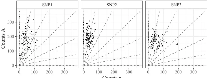
Overdispersion refers to additional variability than expected under a simple model. Overdispersion is a common feature in many datasets. In sequencing experiments, overdispersion could be introduced by variation in the processing of a sample, by variations in a sample’s biochemistry, or by added mea-surement error introduced by the sequencing machine. These could all result in observed read-counts being more dispersed than expected under the simple binomial model (3). Figure 5 (which is an annotated version of the left panel in Figure 3) illustrates overdispersion in these data.

To model overdispersion, we replace the binomial model with a binomial model (Skellam 1948). The beta-binomial model assumes that each individual draws their own individual-speciﬁc mean probability from a beta-distribu-tion, then draws their counts conditional on this probability:

qipi;e;h;t

Beta jðpi;e;hÞ

12t

t ;

12jðpi;e;hÞ

12t t

!

(13)

yini;qi

Binomialðni;qiÞ: (14)

Here jðpi;e;hÞ (12) is the mean of the underlying beta-distribution, and t2 ½0;1 is the overdispersion parameter, with values closer to 0 indicating less overdispersion and values closer to 1 indicating greater overdispersion. (The parameter tcan also be interpreted as the“intraclass correlation”(Crowder 1979)). The q’is are dummy variables representing individual

speciﬁc probabilities, and are integrated out in the following analyses. We denote the marginal distribution ofyias

yini;pi;e;h;t

BBni;jðpi;e;hÞ;t : (15)

Modeling outliers

The right panel of Figure 3 illustrates another important fea-ture of real data: outliers. Here, most of the points appear well-behaved, but one point (marked as a triangle) is far from the remaining points. Furthermore, taking account of the fact that these data came from an S1 population, this outlying point is inconsistent with the other points. This is because the other points strongly suggest that the parental genotype is AAAAAa, meaning that the possible genotypes are AAAAAA, AAAAAa, and AAAAaa, and the triangle lies far from the expectation for any of these genotypes. Indeed, un-der aﬁtted beta-binomial model, if the individual’s genotype were AAAAaa, then the probability of seeing as few or fewer A counts in this individual as were actually observed is 8:731026_{(Bonferroni-corrected}_P_{-value of 0.0012). There}

are many possible sources of outliers like this, including in-dividual-speciﬁc quirks in the ampliﬁcation or read-mapping steps, and sample contamination or mislabeling.

There are several common strategies for dealing with outliers. These include using methods that are inherently robust to outliers (Huber 1964); identifying and removing outliers prior to analysis (Hadi and Simonoff 1993); or mod-eling the outliers directly (Aitkin and Wilson 1980). Here, we take this last approach, which has the advantage of providing measures of uncertainty for each point being an outlier.

Speciﬁcally, we model outliers using a mixture model:

yini;pi;e;h;t;p

pBBni;jðpi;e;hÞ;t

þð12pÞBBðni;1=2;1=3Þ; (16)

(6)

but we found that this can overﬁt the data in some instances; not shown.)

Prior on sequencing error rate and bias parameter

In some cases we found that maximum likelihood estima-tion of the bias parameterhand error rateegave estimates that were unrealistic, and led to undesirable results. For example, we often observed this problem at SNPs where all individuals carry the same genotype (i.e., monomorphic markers).

Figure 6A shows an example of this problem for simu-lated data from an autotetraploid species in which an AAAA parent is crossed with an aaaa parent, which results in all offspring having the same genotype AAaa. Using the model described up to now yields a maximum likelihood estimate of sequencing error rate^e¼0:37;which is unre-alistically high. This further creates very poor genotype calls (Figure 6B).

To avoid this problem, we place priors oneandhto capture the fact thatewill usually be small, andhwill not deviate too far from 1. Speciﬁcally we use

logitðeÞ Nðme;s2eÞ; and (17)

logðhÞ Nmh;s2h (18)

with software defaults me¼ 24:7; s2e ¼1; mh¼0; and s2

h ¼0:7

2_:_{With these defaults, 95% of the prior mass is on}

e2 ½0:0012;0:061 and h2 ½0:25;4:1 (see Supplemental Material, Figure S1 for graphical depictions.). We chose these defaults based on empirical observations (Figure S8), inﬂ at-ing the variances to make the priors more diffuse (less in-formative) than what we observe in practice. Our prior on the sequencing error rate is also consistent with literature estimates from various platforms (Goodwin et al. 2016), though some sequencing technologies can have error rates as high as 15% and, if using such technologies, the prior should be adjusted accordingly.

Ideally, one would incorporate these prior distributions into a full Bayesian model, and integrate over the resulting posterior distribution oneandh. However, this would require nontrivial computation, and we take the simpler approach of simply multiplying the likelihood by the priors (17) and (18) and maximizing this product in place of the likelihood.

(Effectively this corresponds to optimizing a penalized likeli-hood.) SeeModelfor details.

Using both these priors results in accurate genotypes for our simulated example (Figure 6C).

Incorporating parental reads

In genetic studies involving mating designs, researchers al-most always have NGS data on parent(s) as well as offspring. Such data can be easily incorporated into our model.

Speciﬁcally, we model the number of A reads in parentℓ (denoted ~y_ℓ) given the total number of reads in parent ℓ (denotedn~_ℓ) and allelic dosagep_ℓby:

~

y_ℓn~_ℓ;~p_ℓ;e;h;t;p pBB~n_ℓ;j~p_ℓ;e;h ;t

þð12pÞBB~n_ℓ;1=2;1=3 : (19)

We treat the parental read count data as independent of the offspring count data (given the underlying genotypes), so the model likelihood is the product of (19) and (6).

Model

We now summarize our model andﬁtting procedure. Our model is:

yini;pi¼ki=K;e;h;t;p

pBBni;jðki=K;e;hÞ;t þ ð12pÞBB

ni;1=2;1=3 ;

(20)

~

yj~nj;~pj¼ℓj=K;e;h;t;p

pBB~nj;jðℓj=K;e;hÞ;t þ ð12pÞBB

nj;1=2=;1=3

(21)

Xki

j¼0

HG

j;K 2 ℓ1;K

HG

ki2j;

K 2 ℓ2;K

(22)

logitðeÞ N

m_e;s2

e

; (23)

logðhÞ N

m_h;s2 h

: (24)

Toﬁt this model for offspring from two shared parents (an F1 cross), we ﬁrst estimatee,h,t,p,ℓ1, andℓ2 via maximum

likelihood (or, forh;e;the posterior mode):

(7)

arg max ðe;h;t;p;ℓ1;ℓ2Þ2

½0;13ℝþ3½0;13½0;130:K30:K

pðhÞpðeÞ

3pð~y1j~n1;ℓ1=K;e;h;t;pÞpð~y2j~n2;ℓ2=K;e;h;t;pÞ

3Y

i

XK

ki¼0

pðyijni;ki=K;e;h;t;pÞpðki=Kjℓ1=K;ℓ2=KÞ:

(25)

We perform this maximization using an expectation maximi-zation (EM) algorithm, presented in File S1. The M-step (S5) involves a quasi-Newton optimization for each possible com-bination of ℓ1 andℓ2;which we implement using the optim

function in R (R Core Team 2017).

Given estimates^e;h^;^t;p^;^ℓ1;and^ℓ2;we use Bayes’theorem

to obtain the posterior probability of the individuals’ genotypes:

Pr pi¼

ki

K

yi;^e;^h;t^;p^;^ℓ1;^ℓ2 !

¼

p yini;

ki

K;^e;h^;^t;p^ !

Pr pi¼

ki

K ~p1¼

^_ℓ₁

K;~p2¼

^_ℓ₂

K !

PK

ki¼0p yini;ki

K;^e;h^;^t;p^ !

Pr pi¼ki

K ~p1¼

^_ℓ₁

K;~p2¼

^_ℓ₂

K !:

(26)

From this we can obtain, for example, the posterior mean genotype or a posterior mode genotype for each individual. Theuivalues from the E-step in (S2) in File S1 may be inter-preted as the posterior probability that a point is a nonoutlier. Modifying the EM algorithm in File S1 to deal with offspring from an S1 (instead of F1) cross is straightforward: simply constrainℓ1 ¼ℓ2and removepð~y2~n2;ℓ2=K;e;h;t;pÞfrom (25).

This procedure is implemented in the R package updog (using parental data for offspring genotyping).

Screening SNPs

No matter the modeling decisions made, there will likely be poorly behaved SNPs/individuals whose genotypes are

unreliable. Such poorly behaved SNPs/individuals may orig-inate from sequencing artifacts, and it is important to consider identifying and removing them. The Bayesian paradigm we use naturally provides measures of genotyping quality, both at the individual and SNP levels.

Letqibe the maximum posterior probability of individual

i. That is,

qi:¼max

k Prðpi¼ki=Kjyi;^e; ^

h;^t;p^;^ℓ1;^ℓ2Þ; (27)

where the right-hand side of (27) is deﬁned in (26). Then, the posterior probability of an individual being genotyped incorrectly is 12qi; and individuals may beﬁltered based on this quantity. That is, if a researcher wants to have an error rate,0.05 then they would remove individuals with 12qi.0:05: The overall error rate of a SNP is

r:¼12ð1=nÞP_iqi;wherenis the number of individuals in the sample. That is,ris the posterior proportion of individuals genotyped incorrectly at the SNP. Whole SNPs that have a large value ofrmay be discarded.

We evaluate the accuracy ofrinSimulation comparisons to other methods.

Accounting for preferential pairing

(8)

stable autopolyploids (Bomblies et al.2016), and, when it does occur, the levels of double reduction can be relatively low (Stiftet al.2008), and so the method below might act as a reasonable approximation in the presence of multivalent pairing. Another example of Mendelian violations would be distortion resulting from an allele being semilethal.

Preferential pairing describes the phenomenon where some homologous chromosomes are more likely to pair during meiosis. Preferential pairing affects the segregation patterns of haplotypes, and, hence, the distribution of genotypes in a sample. For a good overview of preferential pairing, see Voorrips and Maliepaard (2012).

To begin, we define a particular set of chromosome pairings to be a“pairing configuration.”Again, we suppose that all pairing during meiosis is bivalent. Since chromosomes are not labeled (we are only interested in the counts of reference and alternative alleles, and not the specific chromosome carrying these alleles), we may represent each configuration by a 3-tuplem2ℕ3_;_where

theﬁrst element contains the number of aa pairs, the second element contains the number of Aa pairs, and the third element contains the number of AA pairs. For example, for the two

con-ﬁgurations of a hexaploid parent with three copies of A,

AajaajAA and AajAajAa,

we represent theﬁrst conﬁguration bym¼ ð1;1;1Þand the second bym¼ ð0;3;0Þ:

Given a conﬁgurationm; aK-ploid parent will segregate K=2 chromosomes to an offspring. The counts of reference alleles that segregate to the offspring, which we denote byz, will follow an“off-center”binomial distribution:

½z2m3jm Binðm2;1=2Þ; (28)

since, in aa pairs, no A alleles segregate; in AA pairs, only A alleles segregate; and in Aa pairs, an A allele segregates with probability 1/2. However, the configuration that formsmis a random variable. Suppose there areqðℓÞpossible confi gura-tions [see Theorem S1 in File S1 for deriving qðℓÞ] given a parent hasℓcopies of A. Also suppose configurationmihas probabilitygiof forming. Then the distribution ofzis a mix-ture of (28), with density

pðzjg;ℓÞ ¼X

qðℓÞ

i¼1

g_iBinðz2mi3jmi2;1=2Þ: (29)

The values ofgiin (29) determine the degree and strength of preferential pairing. If there is no preferential pairing, then the segregation probabilities (29) will equal those from the hypergeometric distribution (5). We derive the values ofgi that result in the hypergeometric distribution in Theorem S5 in File S1. Any preferential pairing will result in deviations away from the weights in Theorem S5.

If neither parent in an F1 population exhibits preferential pairing, then the genotype distribution will follow (4). How-ever, deviations from (4) can occur if some bivalent pairings occur with a higher probability than random chance would allow (Theorem S5 in File S1). In which case, the offspring genotype distribution would be a convolution of two densi-ties of family (29). Speciﬁcally, if parent 1 has genotypeℓ1

and conﬁguration probabilitiesg1, and parent 2 has genotype

ℓ2 and conﬁguration probabilitiesg2;then the offspring

ge-notype distribution is

Prðpi¼k=Kjℓ1;g1;ℓ2;g2Þ ¼ XK

i¼0

pðijg1;ℓ1Þpðk2ijg2;ℓ2Þ:

(30)

Allowing for arbitrary levels of preferential pairing is simply replacing prior (4) with (30). We have made this modiﬁcation in updog, where we estimate both the pa-rental genotypes (ℓ1andℓ2) and the degree and strength

of the preferential pairing (g1andg2) by maximum

mar-ginal likelihood.

This model for preferential pairing is similar to that of Stift et al.(2008), although there are major differences: (i) they do not use this model for genotyping, (ii) the chromosomes are not labeled in our setting and are in theirs, and (iii) we allow for arbitrary ploidy levels while they just allow for tetraploidy.

Extension to population studies

We have focused here on data from an F1 (or S1) experimental design, using parental information to improve genotype calls. Figure 5 A genotype plot illustrating overdispersion compared with the

(9)

However, a similar approach can also be applied to other samples (e.g., outbred populations) by replacing the prior on offspring genotypes (4) with another suitable prior. For example, previous studies have used a discrete uniform dis-tribution (McKennaet al.2010), a binomial distribution that results from assuming HWE (Li 2011; Garrison and Marth 2012), and a Balding-Nichols beta-binomial model on the genotypes (Balding and Nichols 1995, 1997) that assumes an individual contains the same overdispersion parameter across loci (Blischaket al.2018). (All of these previous meth-ods use models that are more limited than the one we present here: none of them account for allelic bias, outliers, or locus-speciﬁc overdispersion; and most implementations assume the sequencing error rate is known).

In our software, we have implemented both the uniform and binomial (HWE) priors on genotypes. The former is very straightforward. The latter involves modifying the EM algo-rithm in File S1 by replacingakiℓ1ℓ2in (S1) with the binomial probabilityPrðkijni;aÞ;whereais the allele frequency of A, and then optimizing overða;t;h;eÞin (S5).

Though the uniform distribution might seem like a reason-able “noninformative”prior distribution, in practice it can result in unintuitive genotyping estimates. This is because the maximum marginal likelihood approach effectively esti-mates the allelic biashand sequencing error rateein such a way that the estimated genotypes approximate the assumed prior distribution. As most populations do not exhibit a uni-form genotype distribution, this can result in extreme esti-mates of the bias and sequencing error rates, resulting in poor genotype estimates. We thus strongly recommend against using the uniform prior in practice, and suggest researchers use more ﬂexible prior distributions, such as the binomial prior.

Using oracle results for sampling depth guidelines

In this section, we develop oracle rates for incorrectly geno-typing individuals based on our new likelihood (20). These rates are“oracle”in that they are the lowest achievable by an ideal estimator of genotypes. Using these oracle rates, we provide a method that returns a lower bound on read depths required to get an error rate less than some threshold. This method also returns the correlation of the oracle estimator with the true genotype, which might be useful when choosing the read depths for association studies.

To begin, we suppose that the sequencing error ratee, bias h, overdispersiont, and genotype distributionpðk=KÞare all known. That is, the probability of dosagepi¼k=Kispðk=KÞ: Developing read depth suggestions when these quantities are known will provide lower bounds on the read depths re-quired when they are not known. However, standard maxi-mum likelihood theory guarantees that the following approximations will be accurate for a large enough sample of individuals (even for low read depth).

Given that these quantities are known, we have a simpliﬁed model with a likelihoodpðyijpi¼k=KÞ[deﬁned in (20)] and a prior pðpiÞ;where the only unknown quantity is the allele dosage pi: Under 0/1 loss, the best estimator of pi is the maximuma posteriori(MAP) estimator

bpi¼arg max pi

pðyijpiÞpðpiÞ: (31)

Notice that^piis only a function ofyiand notpi:Thus, under this simpliﬁed model, one can derive the joint distribution of piand^piby summing over the possible countsyi:

Pr

pi¼k=K;bpi¼ℓ=K

¼ X

yi:^piðyiÞ¼ℓ=K

pðyijk=KÞpðk=KÞ:

(32)

Given this joint distribution (32), one can calculate the oracle misclassiﬁcation error rate

Pr

pi6¼bpi

¼12X

K

k¼0

Pr

pi¼k=K;bpi¼k=K

: (33)

One can also calculate the oracle misclassiﬁcation error rate conditioned on the individual’s genotype

Pr

pi6¼bpijpi¼k=K

¼12Pr

pi¼k=K;bpi¼k=KÞ=pðk=KÞ

: (34)

Also possible is calculating the correlation between the MAP estimator and the true genotype. All of these calculations have been implemented in the updog R package.

(10)

number if the sample is from an F1 population), and thenﬁnd the read depths required to obtain the oracle sequencing error rate (33) below some threshold that depends on their domain of application. We provide an example of this in Sampling depth suggestions.

In the machine learning community, Equation (33) is often called the Bayes error rate (Hastieet al.2009, Section 2.4).

Data availability

The methods implemented in this paper are available in the updog R package available on the Comprehensive R Archive Network athttps://cran.r-project.org/package=updog. Code and instructions to reproduce all of the results of this paper (doi:https://doi.org/10.5281/zenodo.1203697) are avail-able at https://github.com/dcgerard/reproduce_genotyping. Supplementalﬁgures, and supplemental text containing opti-mization details, theorems, and proofs, have been deposited at Figshare. Supplemental material available at Figshare:

https://doi.org/10.25386/genetics.7019456.

Results

Simulation comparisons to other methods

We ran simulations to evaluate updog’s ability to estimate model parameters and genotype individuals in hexaploid species. Since most competing methods do not allow for an F1 population of individuals [although see Serang et al. (2012) implemented at https://bitbucket.org/orserang/

supermassa.git], we compared the HWE version of updog

(Extension to population studies), a GATK-like method (here-after, “GATK”) (McKenna et al. 2010) as implemented by updog (by using a discrete uniform prior on the genotypes,

fixinghto 1 andtto 0, while specifyinge),fitPoly (Voorrips et al.2011), and the method of Li (2011) as implemented by Blischak et al.(2018). Other methods are either specific to tetraploids, or only have implementations for tetraploids (Maruki and Lynch 2017; Schmitz Carley et al. 2017), so we did not explore their performances.

Speciﬁcally, we simulated 142 unrelated individuals [the number of individuals in the dataset from Shirasawa et al.

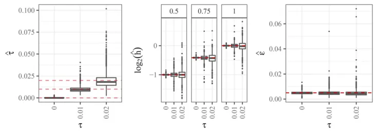
(2017)] under the updog model with sequencing error rate e¼0:005;overdispersion parametert2 f0;0:01;0:02g;and bias parameter h2 f0:5;0:75;1g(withh¼1 indicating no bias). These parameter values were motivated by features in real data (Figure S8). We did not allow for outliers, neither in the simulated data nor in theﬁt. For each combination oft and h, we simulated 1000 datasets. The ni values were obtained from the 1000 SNPs in the Shirasawa et al. (2017) dataset with the largest read-counts. The distribution of the genotypes for each locus was distributed binomially using an allele frequency chosen from a uniform grid from 0.05 to 0.95.

Figure 7 contains boxplots for parameter estimates from the updog model. In general, the parameter estimates are highly accurate for small values of overdispersion and be-come less accurate, though still approximately unbiased, for larger values of overdispersion. The accuracy of the pa-rameter estimates vary gradually for different levels of allele frequencies (Figures S4 and S5). We note that, in real data, only a small fraction of estimates of the overdispersion pa-rameter are higher than 0.02 (Figure S8).

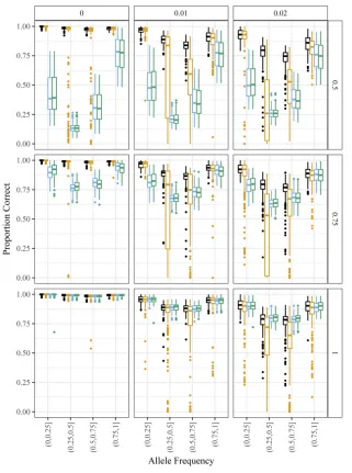
We then compared the genotyping accuracy of updog with the method from Li (2011), GATK (McKennaet al.2010), and

ﬁtPoly (Voorripset al.2011). In Figure 8, we have boxplots of the proportion of samples genotyped correctly stratiﬁed by bins of the allele frequency, color coding by method. We draw the following conclusions:

1. All methods show similar performance when there is no biasðh¼1Þand no overdispersionðt¼0Þ. These are the (unstated) assumptions of GATK and the method of Li (2011).

2. Overdispersion generally makes estimating genotypes much more difﬁcult, and accurate genotyping can only be guaranteed for small levels of overdispersion.

3. When there is any bias, updog has much superior perfor-mance to GATK and the method of Li (2011).

4. ﬁtPoly performs well when there is no overdispersion, even for large levels of bias. However, in the presence of small amounts of overdispersion,ﬁtPoly provides unstable genotype estimates.

Figure 7 Left: Boxplots of estimated overdispersion parameter (y-axis)

strati-ﬁed by the value of overdispersion (x -axis). The horizontal lines are at 0, 0.01, and 0.02. Center: Boxplots of log2-transformed estimates of the bias

(11)

5. Even when there is no bias, updog performs as well as GATK and the method of Li (2011), except for some data-sets where the allele frequency is close to 0.5 and the overdispersion is large. This is because GATK and the method of Li (2011) both effectively assume the bias pa-rameterhis known at 1, while updog is using a degree of freedom to estimate the bias parameter. In the case where there is actually no bias, this can make updog’s estimates somewhat more unstable.

Even though the genotyping results are not encouraging for large amounts of overdispersion, updog has some ability to estimate this level of overdispersion to provide information to researchers on the quality of a SNP (Figure 7).

We compared the allele frequency estimates from updog and the method of Li (2011). Here, the results are more encouraging (Figure S2). Even for large levels of overdis-persion and bias, updog accurately estimates the allele frequency (though less accurately than with small overdispersion). As

expected, the method of Li (2011) is adversely affected by bias, which it does not model, and tends to overestimate the allele frequency in the direction of the bias.

(12)

updog’s posterior means could improve the results of associ-ation studies.

Finally, we compared the ability of updog and ﬁtPoly to estimate the proportion of individuals genotyped incorrectly. Accurate estimates of this quantity can aid researchers when

filtering for high-quality SNPs (Screening SNPs). The software implementation of updog returns this quantity by default, while we derived this quantity fromfitPoly using the output of the posterior probabilities on the genotypes. We subtracted the true proportion of individuals genotyped incorrectly from the estimated proportion and provide boxplots of these quan-tities in Figure 9. Generally, updog provides more accurate estimates for this proportion than fitPoly, particularly for small levels of overdispersion and allele frequencies close to 0.5.

Simulation comparing use of S1 prior and HWE prior

We ran simulations to evaluate the gains in sharing informa-tion between siblings in an S1 populainforma-tion. We drew the

genotypes of an S1 population of 142 individuals where the parent contains either three, four, orﬁve copies of the refer-ence allele. We then simulated these individuals’read-counts under the updog model using the same parameter settings as in Simulation comparisons to other methods: e¼0:005; t2 f0;0:01;0:02g;and h2 f0:5;0:75;1g(with h¼1 indi-cating no bias). For each combination of parental genotype, overdispersion, and allelic bias, we simulated 1000 datasets. Thenivalues were again obtained from the 1000 SNPs in the Shirasawaet al.(2017) dataset with the largest read-counts. For each dataset, weﬁt updog using a prior that either assumes the individuals were from an S1 population (Model) or were in HWE (Extension to population studies). We plot summaries of the proportion of individuals genotyped cor-rectly across datasets on Figure 10. In every combination of parameters, correctly assuming an S1 prior improves per-formance, particularly when there is a small amount of overdispersion (t¼0:01). Boxplots of the proportion of in-dividuals genotyped correctly may be found in Figure S7.

(13)

Simulations on preferential pairing

InAccounting for preferential pairingwe developed a proce-dure to account for arbitrary levels of preferential pairing. In this section, we evaluate the accuracy of updog in the pres-ence of preferential pairing.

We consider a tetraploid S1 population of individuals. In such a population, preferential pairing only affects the seg-regation probabilities when the parent has two copies of the reference allele (because this is the only scenario in a tetra-ploid population where there is more than one pairing

con-figuration—see Theorem S1 in File S1). In this setting, the two possible pairing configurations are m¼ ð1;0;1Þ and m¼ ð0;2;0Þ: Under a nonpreferential pairing setting, the weights of each configuration would beg1¼1=3 for thefirst

conﬁguration andg2¼2=3 for the second (Theorem S5 in

File S1).

To explore the performance of updog in the case of the most extreme levels of preferential pairing possible in a tetraploid species, we simulated offspring genotypes by setting ei-therg1 ¼0 or g1¼1:We did this while settinge¼0:005;

t2 f0;0:01;0:02g; and h2 f0:5;0:75;1g: Figure 11 con-tains boxplots of the estimated levels ofg1against the true

values ofg1:updog can estimateg1 reasonably accurately,

though these estimates become less stable as the overdisper-sion increases.

We compared the preferential-pairing version of updog to

ﬁtPoly and the nonpreferential pairing version of updog. Fig-ure 12 contains boxplots of the proportion of individuals genotyped correctly stratiﬁed byg1:The preferential pairing

version of updog performs better than ﬁtPoly and the non-preferential pairing version of updog, particularly in the pres-ence of large amounts of overdispersion, and when g1 is

large.

Sweet potato

Weﬁt the Balding-Nichols version of the method of Blischak et al. (2018), the method of Serang et al.(2012) (imple-mented in the SuperMASSA software at http://statgen.

esalq.usp.br/SuperMASSA/),ﬁtPoly (Voorripset al.2011),

(14)

error rate to be known, we use the sequencing error rate estimates provided by updog.

FitPoly allows for F1, but not S1, populations, and seem-ingly only when parental counts are provided. To account for this, we copied the read-counts data from the parent and speciﬁed this duplicated point as a second parent. As recom-mended by the authors’ documentation, we ﬁt these data using the try.HW = TRUE setting.

Theﬁts for all four methods can be seen in Figure 13. Our conclusions are:

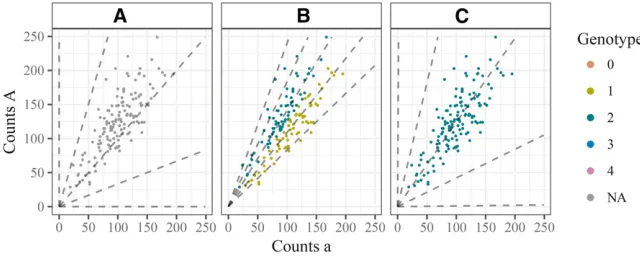
1. Serang et al.(2012) and Blischak et al.(2018) provide unintuitive results for SNP2. As we know this is an S1 population, the genotype distribution should be closer to a 1:2:1 ratio for genotypes AAAAAA, AAAAAa, and AAAAaa. Both updog and ﬁtPoly correctly accounts for this. Updog does so by estimating an extreme bias while

ﬁtPoly does so by allowing the mean proportion of refer-ence counts for each genotype to depend only linearly or quadratically on the dosage level.

2. The method of Serang et al. (2012) was designed for Gaussian, not count, data and, as such, provides some unintuitive genotyping. In particular, for SNPs 1 and 2 we see a few points on the left end of the AAAAAa genotypes that are coded AAAAAA when these could prob-ably only result from an extreme sequencing error rate given that genotype.

3. The point in SNP3 that we have described as an outlier is removed by updog. The other methods are not able to cope with outliers.

(15)

anomalous results byﬁtPoly, as these SNPs seem mostly well-behaved (Figure S10).

Computation time

We measured the computation time required tofit updog to the 1000 SNPs with the highest read depth from the dataset of Shirasawa et al. (2017). These computations were run on a 4.0 GHz quad-core PC running Linux with 32 GB of memory. It took on average 3.3 sec per SNP tofit updog, with 95% of the runs taking between 1.81 and 6.56 sec. This is much larger than the total time of 121 sec it took for the software of Blischaket al. (2018) tofit their model on all 1000 SNPs. But it is almost exactly equal to the computation time offitPoly, where 95% of the runs took between 1.77 and 6.55 sec. Also, since the SNPs in updog arefitted independently, this allows us to easily parallelize this computation over the SNPs.

Sampling depth suggestions

InUsing oracle results for sampling depth guidelines, we de-rived the oracle genotyping error rates given that the

sequencing error rate, the allelic bias, the overdispersion, and the genotype distributions are all known. In this section, we explore these functions in the particular case when a SNP is in HWE with an allele frequency of 0.8.

(16)

many times larger to obtain the same error rates as when there is no bias and no overdispersion.

Though the read depth requirements to obtain a small error rate seem depressing under reasonable levels of bias and overdispersion, the results are much more optimistic to obtain high correlation with the true genotypes. In Figures S14–S16, we calculated the minimum read depths required to obtain a correlation with the true genotypes of.0.9 under the same parameter settings as Figures S11–S13. There, we see that the read depth requirements are much more reasonable, where, for hexaploid species, a read depth of 90 is adequate to obtain this correlation under large levels of bias and over-dispersion. Correspondingly, for tetraploids a read depth of 25 seems adequate to obtain high correlation under large levels of bias and overdispersion.

Once again, we would like to stress that these are lower boundson the read depth requirements. Actual read depths should be slightly larger than these, based on how many individuals are in the study.

Discussion

We have developed an empirical Bayes genotyping procedure that takes into account common aspects of NGS data: se-quencing error, allelic bias, overdispersion, and outlying points. We have shown that accounting for allelic bias is vital for accurate genotyping, and that that our posterior measures of uncertainty (automatically taking into account the esti-mated levels of overdispersion) are well calibrated and may be used as quality metrics for SNPs/individuals. We conﬁrmed the validity of our method on simulated and real data.

We have focused on a dataset that has a relatively large read-coverage and contains a large amount of known struc-ture (via Mendelian segregation). In many datasets, one would expect to have much lower coverage of SNPs and less structure (Blischak et al. 2018). For such data, we do not expect the problems of allelic bias, overdispersion, and out-lying points to disappear. From our simulations, the most in-sidious of these issues to ignore is the allelic bias. If a Figure 13 Genotype plots as in Figure 3 but color-coded by the estimated geno-types from the method of Blischaket al.

(17)

reference genome is available, then it might be possible to correct for the read-mapping bias by using the methods from van de Geijn et al.(2015). However, this might not be the total cause of allelic bias. And, without a reference genome, it is important to model this bias directly. We do not expect small coverage SNPs to contain enough information to accu-rately estimate the bias using our methods. For such SNPs, more work is needed. It might be possible to borrow strength between SNPs to develop accurate genotyping methods.

We have assumed that the ploidy is known and constant between individuals. However, some species (e.g., sugarcane) can have different ploidies per individual (Garciaet al.2013). If one has access to good cytological information on the ploidy of each individual, it would not be conceptually diffi -cult to modify updog to allow for different (and known) ploi-dies of the individuals. However, estimating the ploidy might be more difficult, particularly in the presence of allelic bias. In the presence of such bias, one can imagine that it would be difficult to discern if a sample’s location on a genotype plot was due to bias or due to a higher or lower ploidy level. More work would be needed to develop an approach that works with individuals having unknown ploidy levels. Seranget al. (2012) attempts to estimate the ploidy level in Gaussian data, but they do not jointly account for allelic bias, which we hypothesize would bias their genotyping results.

Garrison and Marth (2012) uses a multinomial likelihood to model multiallelic haplotypes. This allows for more com-plex genotyping beyond SNPs. The models presented here could be easily extended to a multinomial likelihood. For example, to model bias withkpossible alleles, one could in-troducek21 bias parameters which measure the bias of each allele relative to a reference allele. One could use a Dirichlet-multinomial distribution to model overdispersion and a uni-form-multinomial distribution (uniform on the standard k21 simplex) to model outliers. Modeling allele-detection errors (corresponding to sequencing errors in our NGS setup) would be context-speciﬁc.

The methods developed here may also be useful for gen-otyping diploid individuals. We are not aware of diploid genotyping methods that account for allelic bias, overdisper-sion, and outlying points. However, considering our oracle results in Sampling depth suggestions, accounting for these features is probably more important for polyploid species, as determining allele dosage is more difﬁcult than determin-ing heterozygosity/homozygosity.

Genotyping is typically only one part of a large analysis pipeline. It is known that genotyping errors can inﬂate genetic maps (Hackett and Broadfoot 2003), but it remains to de-termine the impact of dosage estimates on other downstream analyses. In principle, one would want to integrate out un-certainty in estimated dosages, but, in diploid analyses, it is much more common to ignore uncertainty in genotypes and simply use the posterior mean genotype—for example, in GWAS analyses (Guan and Stephens 2008). It may be that similar ideas could work well for GWAS in polyploid species (see also Grandkeet al.2016).

Acknowledgments

We sincerely thank the authors of Shirasawa et al. (2017) for providing their data and Paul Blischak for providing use-ful comments. D.G. and M.S. were supported by National Institutes of Health (NIH) grant HG002585 and by a grant from the Gordon and Betty Moore Foundation (Grant GBMF #4559). L.F.V.F. and A.A.F.G. were partially supported by grant 2014/20389-2, FAPESP/CAPES (São Paulo Research Foundation). A.A.F.G. was supported by a productivity scholarship from the National Council for Scientiﬁc and Technological Development (CNPq).

Literature Cited

Aitkin, M., and G. T. Wilson, 1980 Mixture models, outliers, and the EM algorithm. Technometrics 22: 325–331.https://doi.org/ 10.1080/00401706.1980.10486163

Baird, N. A., P. D. Etter, T. S. Atwood, M. C. Currey, A. L. Shiver et al., 2008 Rapid SNP discovery and genetic mapping using sequenced RAD markers. PLoS One 3: e3376.https://doi.org/ 10.1371/journal.pone.0003376

Balding, D. J., and R. A. Nichols, 1995 A method for quantifying differentiation between populations at multi-allelic loci and its implications for investigating identity and paternity, pp. 3–12 in Human Identiﬁcation: The Use of DNA Markers, edited by B. S. Weir. Springer, Berlin.https://doi.org/10.1007/978-0-306-46851-3_2

Balding, D. J., and R. A. Nichols, 1997 Signi_ﬁcant genetic corre-lations among Caucasians at forensic DNA loci. Heredity 78: 583_–589.https://doi.org/10.1038/hdy.1997.97

Bargary, N., J. Hinde, and A. A. F. Garcia, 2014 Finite mixture model clustering of SNP data, pp. 139–157 inStatistical Model-ling in Biostatistics and Bioinformatics: Selected Papers, edited by G. MacKenzie, and D. Peng. Springer International Publishing, New York.https://doi.org/10.1007/978-3-319-04579-5_11

Blischak, P. D., L. S. Kubatko, and A. D. Wolfe, 2016 Accounting for genotype uncertainty in the estimation of allele frequencies in autopolyploids. Mol. Ecol. Resour. 16: 742–754.https://doi. org/10.1111/1755-0998.12493

Blischak, P. D., L. S. Kubatko, and A. D. Wolfe, 2018 SNP geno-typing and parameter estimation in polyploids using low-cover-age sequencing data. Bioinformatics 34: 407–415. https://doi. org/10.1093/bioinformatics/btx587

Bomblies, K., G. Jones, C. Franklin, D. Zickler, and N. Kleckner, 2016 The challenge of evolving stable polyploidy: could an increase in_“crossover interference distance_”play a central role? Chromosoma 125: 287_–300. https://doi.org/10.1007/s00412-015-0571-4

Bourke, P. M., P. Arens, R. E. Voorrips, G. D. Esselink, C. F. S. Koning-Boucoiranet al., 2017 Partial preferential chromosome pairing is genotype dependent in tetraploid rose. Plant J. 90: 330–343.https://doi.org/10.1111/tpj.13496

Bourke, P. M., R. E. Voorrips, R. G. F. Visser, and C. Maliepaard, 2018 Tools for genetic studies in experimental populations of polyploids. Front. Plant Sci. 9: 513. https://doi.org/10.3389/ fpls.2018.00513

Byrne, S., A. Czaban, B. Studer, F. Panitz, C. Bendixen et al., 2013 Genome wide allele frequency ﬁngerprints (GWAFFs) of populations via genotyping by sequencing. PLoS One 8: e57438.https://doi.org/10.1371/journal.pone.0057438

(18)

Clark, L. V., A. E. Lipka, and E. J. Sacks, 2018 polyRAD: genotype calling with uncertainty from sequencing data in polyploids and diploids. bioRxiv 380899.https://doi.org/10.1101/380899. Crowder, M. J., 1979 Inference about the intraclass correlation coefﬁcient in the beta-binomial ANOVA for proportions. J. R. Stat. Soc. B 41: 230–234.

Davey, J. W., P. A. Hohenlohe, P. D. Etter, J. Q. Boone, J. M. Catchenet al., 2011 Genome-wide genetic marker discovery and genotyping using next-generation sequencing. Nat. Rev. Genet. 12: 499–510.https://doi.org/10.1038/nrg3012

Elshire, R. J., J. C. Glaubitz, Q. Sun, J. A. Poland, K. Kawamoto et al., 2011 A robust, simple genotyping-by-sequencing (GBS) approach for high diversity species. PLoS One 6: e19379.

https://doi.org/10.1371/journal.pone.0019379

Garcia, A. A., M. Mollinari, T. G. Marconi, O. R. Serang, R. R. Silva et al., 2013 SNP genotyping allows an in-depth characterisa-tion of the genome of sugarcane and other complex autopoly-ploids. Sci. Rep. 3: 3399.https://doi.org/10.1038/srep03399

Garrison, E., and G. Marth, 2012 Haplotype-based variant detec-tion from short-read sequencing. arXiv:1207.3907v2 [q-bio.GN]. Glaubitz, J. C., T. M. Casstevens, F. Lu, J. Harriman, R. J. Elshire et al., 2014 TASSEL-GBS: a high capacity genotyping by se-quencing analysis pipeline. PLoS One 9: e90346. https://doi. org/10.1371/journal.pone.0090346

Goodwin, S., J. D. McPherson, and W. R. McCombie, 2016 Coming of age: ten years of next-generation sequencing technologies. Nat. Rev. Genet. 17: 333–351. https://doi.org/ 10.1038/nrg.2016.49

Grandke, F., P. Singh, H. C. M. Heuven, J. R. de Haan, and D. Metzler, 2016 Advantages of continuous genotype values over genotype classes for GWAS in higher polyploids: a comparative study in hexaploid chrysanthemum. BMC Genomics 17: 672.

https://doi.org/10.1186/s12864-016-2926-5

Guan, Y., and M. Stephens, 2008 Practical issues in imputation-based association mapping. PLoS Genet. 4: e1000279.https:// doi.org/10.1371/journal.pgen.1000279

Hackett, C., and L. Broadfoot, 2003 Effects of genotyping errors, missing values and segregation distortion in molecular marker data on the construction of linkage maps. Heredity 90: 33–38.

https://doi.org/10.1038/sj.hdy.6800173

Hadi, A. S., and J. S. Simonoff, 1993 Procedures for the identiﬁ -cation of multiple outliers in linear models. J. Am. Stat. Assoc. 88: 1264–1272.https://doi.org/10.1080/01621459.1993.10476407

Hastie, T., R. Tibshirani, and J. Friedman, 2009 The Elements of Statistical Learning. Springer-Verlag, New York.https://doi.org/ 10.1007/978-0-387-84858-7

Huber, P. J., 1964 Robust estimation of a location parameter. Ann. Math. Stat. 35: 73_–101.https://doi.org/10.1214/aoms/1177703732

Kim, C., H. Guo, W. Kong, R. Chandnani, L.-S. Shuang et al., 2016 Application of genotyping by sequencing technology to a variety of crop breeding programs. Plant Sci. 242: 14_–22.

https://doi.org/10.1016/j.plantsci.2015.04.016

Li, H., 2011 A statistical framework for SNP calling, mutation discovery, association mapping and population genetical param-eter estimation from sequencing data. Bioinformatics 27: 2987– 2993.https://doi.org/10.1093/bioinformatics/btr509

Li, X., Y. Wei, A. Acharya, Q. Jiang, J. Kanget al., 2014 A satu-rated genetic linkage map of autotetraploid alfalfa (Medicago sativa L.) developed using genotyping-by-sequencing is highly syntenous with theMedicago truncatulagenome. G3 (Bethesda) 4: 1971–1979.https://doi.org/10.1534/g3.114.012245

Li, Y., C. Sidore, H. M. Kang, M. Boehnke, and G. R. Abecasis, 2011 Low-coverage sequencing: implications for design of complex trait association studies. Genome Res. 21: 940_–951.

https://doi.org/10.1101/gr.117259.110

Liu, H., X. Luo, L. Niu, Y. Xiao, L. Chenet al., 2017 Distant eQTLs and non-coding sequences play critical roles in regulating gene

expression and quantitative trait variation in maize. Mol. Plant 10: 414–426.https://doi.org/10.1016/j.molp.2016.06.016

Lu, F., A. E. Lipka, J. Glaubitz, R. Elshire, J. H. Cherney et al., 2013 Switchgrass genomic diversity, ploidy, and evolution: novel insights from a network-based SNP discovery protocol. PLoS Genet. 9: e1003215.https://doi.org/10.1371/journal.pgen.1003215

Maruki, T., and M. Lynch, 2017 Genotype calling from popula-tion-genomic sequencing data. G3 (Bethesda) 7: 1393–1404.

https://doi.org/10.1534/g3.117.039008

McCallum, S., J. Graham, L. Jorgensen, L. J. Rowland, N. V. Bassil et al., 2016 Construction of a SNP and SSR linkage map in autotetraploid blueberry using genotyping by sequencing. Mol. Breed. 36: 41.https://doi.org/10.1007/s11032-016-0443-5

McKenna, A., M. Hanna, E. Banks, A. Sivachenko, K. Cibulskiset al., 2010 The genome analysis toolkit: a MapReduce framework for analyzing next-generation DNA sequencing data. Genome Res. 20: 1297–1303.https://doi.org/10.1101/gr.107524.110

Mollinari, M., and O. Serang, 2015 Quantitative SNP genotyping of polyploids with MassARRAY and other platforms, pp. 215– 241 in Plant Genotyping: Methods and Protocols, edited by J. Batley. Springer, New York. https://doi.org/10.1007/978-1-4939-1966-6_17

Motazedi, E., D. de Ridder, R. Finkers, S. Baldwin, S. Thomson et al., 2018 TriPoly: haplotype estimation for polyploids using sequencing data of related individuals. Bioinformatics.https:// doi.org/10.1093/bioinformatics/bty442

Nielsen, R., J. S. Paul, A. Albrechtsen, and Y. S. Song, 2011 Genotype and SNP calling from next-generation sequencing data. Nat. Rev. Genet. 12: 443–451.https://doi.org/10.1038/nrg2986

Otto, S. P., and J. Whitton, 2000 Polyploid incidence and evolu-tion. Annu. Rev. Genet. 34: 401_–437.https://doi.org/10.1146/ annurev.genet.34.1.401

Peterson, B. K., J. N. Weber, E. H. Kay, H. S. Fisher, and H. E. Hoekstra, 2012 Double digest RADseq: an inexpensive method for de novo SNP discovery and genotyping in model and non-model species. PLoS One 7: e37135.https://doi.org/10.1371/ journal.pone.0037135

Pritchard, J. K., and M. Przeworski, 2001 Linkage disequilibrium in humans: models and data. Am. J. Hum. Genet. 69: 1–14.

https://doi.org/10.1086/321275

R Core Team, 2017 R: A Language and Environment for Statistical Computing. R Foundation for Statistical Computing, Vienna. Schilling, M. P., P. G. Wolf, A. M. Duffy, H. S. Rai, C. A. Roweet al.,

2014 Genotyping-by-sequencing for populus population geno-mics: an assessment of genome sampling patterns andﬁltering approaches. PLoS One 9: e95292. https://doi.org/10.1371/ journal.pone.0095292

Schmitz Carley, C. A., J. J. Coombs, D. S. Douches, P. C. Bethke, J. P. Paltaet al., 2017 Automated tetraploid genotype calling by hierarchical clustering. Theor. Appl. Genet. 130: 717_–726.

https://doi.org/10.1007/s00122-016-2845-5

Serang, O., M. Mollinari, and A. A. F. Garcia, 2012 Efﬁcient exact maximum a posteriori computation for Bayesian SNP genotyp-ing in polyploids. PLoS One 7: e30906. https://doi.org/10. 1371/journal.pone.0030906

Shirasawa, K., M. Tanaka, Y. Takahata, D. Ma, Q. Cao et al., 2017 A high-density SNP genetic map consisting of a com-plete set of homologous groups in autohexaploid sweetpotato (Ipomoea batatas). Sci. Rep. 7: 44207.

Skellam, J. G., 1948 A probability distribution derived from the binomial distribution by regarding the probability of success as variable between the sets of trials. J. R. Stat. Soc. B 10: 257–261. Soltis, D. E., C. J. Visger, and P. S. Soltis, 2014 The polyploidy revolution then_{. . .}and now: Stebbins revisited. Am. J. Bot. 101: 1057_–1078.https://doi.org/10.3732/ajb.1400178

(19)

Sci. USA 97: 7051–7057. https://doi.org/10.1073/pnas.97. 13.7051

Spindel, J., M. Wright, C. Chen, J. Cobb, J. Gage et al., 2013 Bridging the genotyping gap: using genotyping by se-quencing (GBS) to add high-density SNP markers and new value to traditional bi-parental mapping and breeding popula-tions. Theor. Appl. Genet. 126: 2699–2716 [corrigenda: Theor. Appl. Genet. 129: 201–202 (2016)].https://doi.org/10.1007/ s00122-013-2166-x

Spindel, J., H. Begum, D. Akdemir, P. Virk, B. Collard et al., 2015 Genomic selection and association mapping in rice (Oryza sativa): effect of trait genetic architecture, training population composition, marker number and statistical model on accuracy of rice genomic selection in elite, tropical rice breeding lines. PLoS Genet. 11: 1–25.https://doi.org/10.1371/journal.pgen.1004982

Stebbins, G. L., 1947 Types of polyploids: their classiﬁcation and signiﬁcance, pp. 403–429 inAdvances in Genetics, Vol. 1, edited by M. Demerec. Academic Press, New York. https://doi.org/ 10.1016/S0065-2660(08)60490-3

Stift, M., C. Berenos, P. Kuperus, and P. H. van Tienderen, 2008 Segregation models for disomic, tetrasomic and interme-diate inheritance in tetraploids: a general procedure applied to rorippa(yellow cress) microsatellite data. Genetics 179: 2113– 2123.https://doi.org/10.1534/genetics.107.085027

Stift, M., R. Reeve, and P. H. Van Tienderen, 2010 Inheritance in tetraploid yeast revisited: segregation patterns and statistical power

under different inheritance models. J. Evol. Biol. 23: 1570–1578.

https://doi.org/10.1111/j.1420-9101.2010.02012.x

Tennessen, J. A., R. Govindarajulu, T.-L. Ashman, and A. Liston, 2014 Evolutionary origins and dynamics of octoploid strawberry sub-genomes revealed by dense targeted capture linkage maps. Genome Biol. Evol. 6: 3295–3313.https://doi.org/10.1093/gbe/evu261

Udall, J. A., and J. F. Wendel, 2006 Polyploidy and crop improve-ment. Crop Sci. 46: S3–S14.https://doi.org/10.2135/cropsci2006. 07.0489tpg

van de Geijn, B., G. McVicker, Y. Gilad, and J. K. Pritchard, 2015 WASP: allele-speci_ﬁc software for robust molecular quantitative trait locus discovery. Nat. Methods 12: 1061_– 1063.https://doi.org/10.1038/nmeth.3582

Voorrips, R. E., and C. A. Maliepaard, 2012 The simulation of meiosis in diploid and tetraploid organisms using various genetic models. BMC Bioinformatics 13: 248.https://doi.org/10.1186/ 1471-2105-13-248

Voorrips, R. E., G. Gort, and B. Vosman, 2011 Genotype calling in tet-raploid species from bi-allelic marker data using mixture models. BMC Bioinformatics 12: 172.https://doi.org/10.1186/1471-2105-12-172

Zhou, B., and A. S. Whittemore, 2012 Improving sequence-based genotype calls with linkage disequilibrium and pedigree infor-mation. Ann. Appl. Stat. 6: 457–475.https://doi.org/10.1214/ 11-AOAS527