Hybrid
ab initio
Kohn-Sham density functional theory/frozen-density
orbital-free density functional theory simulation method suitable
for biological systems
Miroslav Hodaka兲
Center for High Performance Simulation and Department of Physics, North Carolina State University, Raleigh, North Carolina 27695-7518, USA
Wenchang Lu and J. Bernholc
Center for High Performance Simulation and Department of Physics, North Carolina State University, Raleigh, North Carolina 27695-7518, USA and CSMD and CNMS, Oak Ridge National Laboratory, Oak Ridge, Tennessee 37831-6367, USA
共Received 13 September 2007; accepted 25 October 2007; published online 2 January 2008兲
A hybrid computational method intended for simulations of biomolecules in solution is described. The ab initio Kohn-Sham 共KS兲 density functional theory 共DFT兲 method is used to describe the chemically active part of the system and its first solvation shells, while a frozen-density orbital-free 共FDOF兲DFT method is used to treat the rest of the solvent. The molecules in the FDOF method have fixed internal structures and frozen electron densities. The hybrid method provides a seamless description of the boundary between the subsystems and allows for the flow of molecules across the boundary. Tests on a liquid water system show that the total energy is conserved well during molecular dynamics and that the effect of the solvent environment on the KS subsystem is well described. An initial application to copper ion binding to the prion protein is also presented. ©2008 American Institute of Physics.关DOI:10.1063/1.2814165兴
I. INTRODUCTION
Ab initiodensity functional theory1 共DFT兲 calculations, originally formulated by Kohn and Sham,2 are widely used for computational investigations of a variety of systems. With the recent improvements in algorithms and computing power, the Kohn-Sham共KS兲DFT can treat systems contain-ing several hundreds of atoms. This, however, is still not enough for studies on biological systems consisting of many thousands of atoms. Such systems are usually treated using classical molecular dynamics with force fields, but such simulations cannot accurately describe chemical processes such as bond breaking, bond creation, or charge transfer.
Of particular interest for biological systems is the treat-ment of solvent molecules. The solvent molecules can either be treated explicitly or implicitly. In implicit methods, the solvent is represented as a polarizable continuum dielectric.3–5The attractiveness of this approach stems from the fact that in many biosimulations, solvent molecules out-number the solute and thus implicit modeling of the solvent can substantially improve the efficiency of simulations. This approach was successfully used6–9 in many instances, but evidence suggests that for a complete understanding of the behavior of many biological systems, an explicit treatment of the solvent is essential. For example, molecular mechanics simulations of proteins have shown that an implicit represen-tation of the solvent leads to incorrect predictions of native structures and folding pathways, while explicit treatment of the solvent yields results in agreement with experimental
observation.10,11Also, for many solvated biomolecules, water molecules are located near the active sites and are essential to their functions. To properly describe such water mol-ecules, hydrogen bonds with other water molecules have to be included and this can only be done when the solvent is treated explicitly.
Inab initiosimulations, it is not feasible to represent the solvent explicitly and thus implicit solvation is often used. The polarizable continuum model12,13is particularly popular. Explicit description of the solvent can only be used when the solvent molecules are represented in an efficient manner, such as at a lower level of theory than the solute. The
quan-tum molecular 共QM兲/molecular mechanics 共MM兲
method,14–16 which combines ab initio and classical force field simulations, is often used to achieve full explicit solva-tion in studies on biomolecules. In this method, the chemi-cally active part of the system is treated at theab initiolevel, while the rest of the system, including the solvent and the remainder of the solute, is treated with classical force field methods. The weak point of QM/MM schemes is the treat-ment of the interaction between the QM and MM sub-systems. A special energy term is required to describe this interaction. This term usually employs force field param-eters, which were developed and tested in calculations within classical molecular mechanics and not for interactions be-tween the QM and MM subsystems. Furthermore, to allow for the flow of solvent molecules across the QM/MM inter-face, resulting in exchange of molecules between the sub-systems, buffer regions and force smoothing functions have to be used.17
In this paper, we explore a different approach to hybrid
a兲Electronic mail: [email protected].
simulation: combining two density functional methods. The chemically active part of the system is treated with the usual ab initio Kohn-Sham DFT, while a frozen-density orbital-free 共FDOF兲 DFT method, which scales linearly with the number of atoms, is used for the rest of the system. In this method, the solvent molecules are assumed to have rigid geometries and frozen electron densities. The advantage of combining two DFT methods is that interactions between the subsystems can be treated at the quantum level rather than at the level of molecular mechanics, as is usually the case in QM/MM methods. In addition, the KS/FDOF hybrid method provides seamless integration between the subsystems and allows for the flow of the molecules across the KS/FDOF interface without the need for a buffer region or force smoothing. Within the KS/FDOF method, energy conserving molecular dynamics simulations can be run even when mol-ecules are exchanged between the subsystems. Tests on liq-uid water at ambient conditions show that KS water mol-ecules have appropriate dipole moments, proving that the effects of the solvent environment are well described. As an example of a realistic application, the KS/FDOF method is used to study copper ion binding to the prion protein. It is found that improved description of solvation effects leads to refinement of the binding site geometry.
This paper is organized as follows: Section II defines the frozen-density orbital-free DFT method and Sec. III de-scribes its application and tests on a homogeneous system of liquid water. In Secs. IV and V, the hybrid KS/FDOF method is formulated and its implementation is discussed. Sections VI and VII present applications to liquid water and to copper ion binding to the prion protein. Finally, Sec. VIII gives the summary and conclusions.
II. FROZEN-DENSITY ORBITAL-FREE DFT SIMULATION METHOD
The KS energy functional is usually written as
E关兴=T关兴+EH关兴+EXC关兴+EAe关兴+EAA, 共1兲
where is the charge density, T关兴 is the noninteracting kinetic energy共KE兲functional,EH关兴is the Hartree energy, EXC关兴 is the exchange-correlation energy, EAe关兴 is the
atom-electron interaction energy, and EAA is the energy of interaction between atoms. By introducing a set of orbitalsi satisfying
=
兺
i兩i兩2 共2兲
and defining kinetic energy as
T关兴= −1 2
兺
i具i兩ⵜ2兩i典, 共3兲
the ground state electron density can be obtained by solving a set of single-particle 共Kohn-Sham兲 equations for orbitals
i. The introduction of orbitals, while very successful, makes the KS DFT calculations computationally demanding: The orbitals have to be evaluated, stored, and kept orthogonal throughout the calculation. Because of this, there has been an interest in developing orbital-free 共OF兲 DFT methods. The
orbital-free approaches eliminate orbitals and attempt to find density by directly minimizing the energy functional. These methods are significantly more efficient than the KS ap-proach and scale linearly with the system size. They can thus be used to study much larger systems than orbital-based methods.
An OF DFT requires that the KE functional in Eq. 共1兲 depends explicitly on the charge density . The simplest such functional is the Thomas-Fermi18–20共TF兲KE functional
TTF=CTF
冕
⍀
5/3共r兲dr, 共4兲
where CTF is 103共32兲2/3 and ⍀ denotes the volume of the
simulation cell. The von Weizsacker KE functional21 adds the dependence on the gradient of charge density to the TF formula:
TW=TTF+
1 1 8
冕
⍀兩ⵜ共r兲兩2
共r兲 dr, 共5兲
where is a constant. For= 9, the TWis the second-order gradient expansion of the Thomas-Fermi KE functional, but other values are also used.22 These functionals, however, yield poor results for the ground state charge density.23 Vari-ous approaches for designing better KE functionals have been suggested, but a highly accurate form of the KE re-mains elusive. Following the success of the generalized-gradient approximation 共GGA兲 approach in exchange-correlation energy functional, a lot of effort24–29 went into the development of GGA KE functionals. For example, Lee et al.28formulated a KE functional共LLP functional兲which is an equivalent of the B88 共Ref. 30兲 exchange-correlation functional,
TLLP=CTF
冕
⍀
5/3
冉
1 + 0.0045x 21 + 0.0253xsinh−1x
冊
dr, 共6兲where
x= 21/3兩ⵜ共r兲兩
4/3共r兲. 共7兲
While the GGA approach improved the quality of OF KE functionals, the obtained ground state charge densities are still not satisfactory.23 Using the nonlocal density approximation,31–35 even more accurate OF KEs have been obtained. These, however, break23 linear scaling of the OF DFT, thus limiting the system sizes to which they can be applied.
Barker and Sprik40used it to study liquid water, and recently Huang and Carter41used it to study Cu and Co atoms on the 共111兲surface of Cu.
To efficiently treat interactions between electrons and atoms, it is desirable to make use of pseudopotentials. The ab initiopseudopotentials42–44 used in KS DFT calculations contain terms dependent on angular momentum that are ap-plied to the KS orbitals. Most of the currently used KS pseudopotentials, such as the Kleinman-Bylander45 or Vanderbilt ultrasoft pseudopotentials,46 are usually of sepa-rable type, i.e., they are written as a sum of a short-range angular-dependent nonlocal part and a long-range spherically symmetric local part. Since the nonlocal part acts on the orbitals of a system rather than on its density, these pseudo-potentials cannot be directly used in OF methods. To enable use of the pseudopotentials in OF methods, one of two ap-proaches is typically used:共i兲Special local pseudopotentials that are directly applicable to charge density are generated47,48 or 共ii兲 existing orbital-based pseudopotentials are used by defining orbitals corresponding to the charge density49–51 共usually a single orbital=1/2is used兲. In our
model, the standard orbital-based pseudopotentials are uti-lized, but only their local parts are applied. Neglecting the nonlocal contributions is well justified because the present model only deals with intermolecular interactions and the short-range nonlocal effects are negligible at typical intermo-lecular distances.
The total electronic energy functional for the present FDOF DFT model is thus
EFDOF关兴=TOF关兴+EH关兴+EXC关兴+EPPlocal关兴+EAA,
共8兲
where TOF stands for any of the OF KE functionals
men-tioned above andEPP
localevaluates the energy of interaction between the electrons and the local part of the pseudopottials. This expression is formally very similar to the KS en-ergy functional, Eq.共1兲. The only differences are the type of the KE functional and the fact that the FDOF method only uses the local part of the pseudopotentials.
The implementation of the FDOF method was based on previously existing KS DFT real-space code52–54 with multi-grid acceleration. This code is well tested and exhibits excel-lent performance on massively parallel supercomputers. In particular, the multigrid Hartree solver and the functions that calculate exchange-correlation and local pseudopotential en-ergies were utilized directly in our implementation. The
RATTLEalgorithm55 was used to keep intramolecular geom-etries fixed.
III. APPLICATION OF FROZEN-DENSITY ORBITAL-FREE DFT METHOD TO LIQUID WATER
Water is the most ubiquitous solvent. In particular, its effects must be accounted for when studying biological sys-tems. In fact, in many biosimulations, the number of atoms in the solvent is much higher than the number of atoms in the solute. It is therefore attractive to formulate a FDOF DFT calculation that would allow for an efficient and accurate treatment of liquid water.
The geometry of water molecules used in the present FDOF method was obtained from KS DFT simulation of liquid water at 300 K. The distance between the oxygen and hydrogen atoms in a water molecule was found to be 0.98 Å and the HOH angle was 105.1°. These values are very close to previously reported KS DFT results:56 rOH= 0.991 Å,
⬔HOH = 105.5°.
For parametrization of the charge density of a water mol-ecule, a functional form proposed by Barker and Sprik40 is used—Gaussians centered on atoms in the molecule. For simplicity, one Gaussian per atom is used. The charge den-sity of a water molecule is then
H2O共r兲=G共qO,␣O,RO,r兲+G共qO,␣O,RH1,r兲
+G共qO,␣O,RH2,r兲, 共9兲
whereGis a Gaussian function centered at the atomic posi-tionR,
G共q,␣,R,r兲=q
冉
␣
冊
3/2
exp共−␣兩r−R兩2兲. 共10兲
This leaves four parameters that need to be determined for the water molecule: the charges on the oxygen and the hy-drogen 共qOand qH兲 and the Gaussian widths 共␣O and␣H兲. The atomic charges can be determined from the total mo-lecular charge and dipole moment. When using pseudopoten-tials, the total charge of a water molecule is 8 and, therefore,
qO+ 2qH= 8. 共11兲
An important characteristic of a water molecule is its dipole moment. In gas phase, its value57 is 1.85 D, but in liquid phase, it increases significantly. The correct value is still under discussion and the estimates range from 2.6 to 3.15 D.58–61 In this work, a value of 3.0 D is used, which is close to the value of 2.95 D obtained from KS DFT studies.56,62Because the electron density is given by Gauss-ians, the dipole moment only depends on the oxygen and hydrogen chargesqOandqHand not on the Gaussian widths.
This gives the second condition for the charges and using the chosen value of 3.0 D for the dipole moment, qO becomes
7.05 electrons andqHbecomes 0.475 electron.
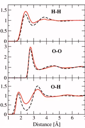
To adjust the Gaussian widths, molecular dynamics simulations were run on a system of 432 water molecules at 300 K. The radial distribution functions共RDFs兲were calcu-lated for various values of parameters ␣Oand␣Hand com-pared to the experimental RDFs.63Using the PBE exchange-correlation potential64,65 and Vanderbilt ultrasoft pseudopotentials,46 various types of KE functionals were also tested. It was found that the LLP functional and values of ␣O= 0.75 and ␣H= 0.8 reproduce the experimental RDFs
complex models of water can be formulated, which would further improve the agreement with experiment.
IV. KS DFT/FDOF DFT HYBRID METHOD
The energy functionals for KS and FDOF DFTs, Eqs.共1兲 and共8兲, are only different in the type of KE functional and the fact that the FDOF method does not use the nonlocal pseudopotential energy. Because of this similarity, it is rela-tively easy to write an expression for the total electronic energy of a hybrid KS DFT/FDOF DFT system.
To do this, consider a system that contains two types of atoms: those that are treated with the FDOF method共FDOF atoms兲and those that are treated with the KS DFT method 共KS atoms兲. The FDOF atoms have fixed charge density FDOF共r兲 attached to them, while the charge density corre-sponding to the KS atoms, KS共r兲, minimizes the energy
functional for the hybrid system. The total charge density of the entire system is simply the sum of both densities,
tot共r兲=FDOF共r兲+KS共r兲. 共12兲
Since the Hartree and exchange-correlation energies are explicit functions of the charge density, it is straightforward to calculate these quantities for the hybrid system usingtot.
The atom-atom interaction energy is also straightforward, be-ing the sum over all atoms present in the hybrid system, regardless of their type. As for the pseudopotential energy, the local and nonlocal parts are treated differently: Each atom has a local potential associated with it and it acts on the total density tot, while only the KS atoms have nonlocal
potentials associated with them and these only act on the KS orbitals.
Defining KE of the hybrid system is somewhat more
complicated. Taking the sum of the FDOF and KS KEs is not sufficient, since kinetic energies are nonadditive. The nonad-ditive part of KE can be estimated38 as
Tnadd关FDOF,KS兴=TOF关tot兴−TOF关FDOF兴−TOF关KS兴.
共13兲
In this and the following formulas, the spatial coordinates are omitted for clarity.
This gives the following functional for the total electron energy of a hybrid system:
Ehybrid关FDOF,KS,兵Ri其FDOF,兵Ri其KS兴
=TTF关TF兴+TKS关KS兴+Tnadd关FDOF,KS兴+EH关tot兴
+EXC关tot兴+EPPnonloc关KS,兵Ri其KS兴+EPPloc关tot,兵Ri其兴
+EAA关兵Ri其兴. 共14兲
Here兵Ri其denotes all atoms in the system and兵Ri其KSstands
for atoms treated by the KS DFT. Note that in this functional, FDOFis rigidly tied to the positions of FDOF atoms, while
KS is determined by minimizing the energy functional
above.
To find the KS ground state charge densityKS, a system
of Kohn-Sham-like equations for orbitals has to be solved,
共
−12ⵜ2+veff兲
i=⑀ii, 共15兲 whereveff= ␦
␦˜KS兵Tnadd关FDOF,˜KS兴+EH关˜KS+FDOF兴 +EXC关˜KS+FDOF兴+EPPnonloc关KS,兵Ri其KS兴
+EPPloc关tot,兵Ri其兴其˜
KS=KS. 共16兲
The effective potential entering Eq.共15兲is thus
veff=vnadd关FDOF,KS兴+vH关tot兴+vXC关tot兴
+vPP关兵Ri其KS兴+vPPloc关兵Ri其FDOF兴=vOF关tot兴
−vOF关KS兴+
冕
tot共r
⬘
兲兩r−r
⬘
兩dr⬘
+vXC关tot兴+vPP关兵Ri其KS兴+vPPloc关兵Ri其FDOF兴, 共17兲
where
vOF关兴=
冏
␦TOF关˜兴
␦˜
冏
˜=共18兲
and vPP without an additional index denotes both local and
nonlocal parts of the pseudopotential. This effective potential is similar to that in the KS DFT theory, the differences being the kinetic energy potential terms, the local pseudopotential due to FDOF atoms, and the fact that the Hartree and exchange-correlation potentials are evaluated using the total charge density rather than the KS density.
V. IMPLEMENTATION OF THE HYBRID METHOD
Hybrid calculation schemes take advantage of the fact that chemical processes in biological systems are usually
well localized. It should therefore be sufficient to treat only a small region of the whole system at a high level of theory. The hybrid KS/FDOF method, as defined in the previous section, has no partitioning between regions and KS or FDOF atoms can coexist anywhere in the simulation cell. However, for this method to be useful for biological simula-tions, the KS atoms have to be restricted to a part of the whole simulation cell.
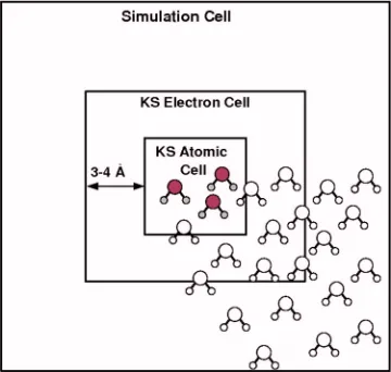
To accomplish this, a region at the center of the total simulation cell, called the KS atomic cell, is defined. This cell holds all KS atoms. The KS density is restricted to the KS electron cell; this cell is typically larger by 3 – 4 Å in each direction than the KS atomic cell to allow for the KS charge density to decrease smoothly to zero at the boundary of the electron cell. The total simulation cell is usually peri-odic. There is no restriction on its size other than it has to be large enough so that biologically relevant molecules located in the KS atomic cell do not interact with their periodic images. We typically use a total cell that is at least 7 Å larger in each direction than the KS electron cell. The layout of the subcells is shown in Fig.2. Note that OF solvent molecules can appear anywhere in the simulation cell, although usually only the first few shells of the solvent molecules closest to the active site are treated by KS DFT and the rest of the solvent molecules is treated by FDOF DFT. In this case, the KS atomic cell can contain both KS and FDOF atoms. An-other possibility, used typically for test simulations on liquid water, is that all solvent molecules completely inside the KS atomic cell are treated by KS DFT and all the rest by FDOF DFT.
The present hybrid method allows for varying the num-ber of solvent molecules treated by the KS method during the course of simulation. Being able to deal with a change in the number of KS atoms is important, since in dynamical calculations, the number of solvent molecules in first solva-tion shells or within the KS atomic cell can change. It is also possible that a solvent molecule originally treated by the KS method moves out of the KS atomic cell. Such molecule
cannot be treated by the KS DFT anymore, since it is re-quired that all KS atoms are inside the KS atomic cell, and the number of KS atoms has to be decreased. When such an event occurs, the KS/FDOF simulation can readily continue, since the total electron energy in the KS/FDOF system关Eq.
共14兲兴 can be calculated for any number of KS and FDOF molecules. However, the exchange causes discontinuities in the total electron energy due to the fact that the electron energy of a solvent molecule is different when calculated with KS or FDOF methods. These discontinuities and the way to restore energy conservation in the simulation will be discussed in the next section.
The hybrid method was implemented to work with both norm-conserving and ultrasoft pseudopotentials共PPs兲. Using ultrasoft PPs in real-space orbital-based DFT methods54 re-quire significant changes compared to using the norm-conserving ones. In particular, ultrasoft PPs require different grids for the charge density and the KS orbitals, while only one global grid is sufficient when norm-conserving PPs are utilized. Accordingly, in the hybrid KS/FDOF method, the KS part uses one or two global grids depending on the type of pseudopotential used. The FDOF part, which deals with charge density only, uses one grid regardless of the type of pseudopotential. To allow for simple transfers between the KS and FDOF grids, it is important that these grids are re-lated. This relationship depends on the PP type: for norm-conserving PPs, the KS and FDOF grids are the same, while for ultrasoft PPs, the FDOF grid is the same as the KS grid used for representing KS orbitals. This means that when the ultrasoft PPs are used, KS and FDOF densities are repre-sented on different grids. The reason for this is efficiency: In ultrasoft KS real-space calculations, the charge density is typically represented on a very fine grid. Using such a grid in the FDOF part would be inefficient and, therefore, the KS orbital grid, which is less dense than the charge density grid, is used. The KS ultrasoft code54 contains functions that in-terpolate between the two grids and, therefore, even when the grids for the charge densities in KS and FDOF parts are different, the quantities represented on one of the grids can be easily transferred to the other.
It should be noted that the present formulation of the hybrid method cannot treat biomolecules that do not fit in-side the KS atomic box, since the FDOF method is currently limited to solvent molecules. This limitation is practical rather than principal, since at present, only parameters for water molecules are determined. It is possible and even likely that a frozen-density parametrization will be devel-oped for biomolecular fragments enabling the treatment of large systems. Although at present only fragments of biomol-ecules with no more than a few hundred atoms can be used in the KS/FDOF DFT simulations, most chemical processes involving creating or breaking of bonds are usually well lo-calized and representing biomolecules by such fragments is often justified. Furthermore, in a typical biosimulation, water molecules constitute a large fraction of the entire simulation system. Therefore, using the FDOF method to treat only the solvent molecules saves substantial computational effort and enables studies of much larger systems.
Finally, it should be mentioned that our embedding
scheme is formally similar to that previously proposed by Wesolowskiet al.38,69,70While they also used frozen density for a part of the system and formulated a calculation scheme combining two DFT methods, the details of the methods are substantially different: Wesolowski et al. employed the so-called “freeze and thaw” procedure in which the two sub-systems in the calculation were periodically frozen and thawed and until convergence was reached. Our frozen-density orbital-free approach allows for more efficient treat-ment of the molecules in the fixed region while still treating all the interactions at the DFT level.
VI. APPLICATION TO LIQUID WATER
An important question for the hybrid method is whether an environment of FDOF water molecules can emulate that of real water molecules. To test this, we run a hybrid simu-lation on a system of 64 water molecules at liquid density at ambient conditions, in which one water molecule was treated by KS DFT and the remaining 63 water molecules were treated by OF DFT. As mentioned above, in the liquid phase, the dipole moment of a water molecule increases from 1.85 D in the gas phase to a value close to 3 D. The value of the dipole moment of the KS molecule during the simulation is plotted in Fig. 3. It varies from 2.23 to 3.54 D and its average value is 2.85 D, which is within the expected range of 2.6– 3.15 D mentioned above. This value is also close to the KS DFT value56,62of 2.95 D.
The ability of the KS/FDOF DFT hybrid method to per-form molecular dynamics simulation is also tested. A system of 432 water molecules at the liquid density at ambient con-ditions is used. The simulation cell and the internal subcells were all cubes with sides of 23.8 Å for the whole simulation cell, 11.9 Å for the KS electron box, and 6.0 Å for the KS atomic box. All the molecules completely inside the KS atomic box are treated by the KS DFT. During the course of the simulation, the number of such molecules charges be-tween 4 and 7. The time step is 0.4 fs and the equations of motions are integrated using second-order Verlet velocity scheme. Ultrasoft pseudopotentials46 are employed and five Nosé-Hoover thermostats are used to maintain the
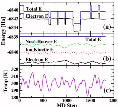
tempera-ture of the system at 300 K. This test simulation confirms that FDOF DFT is indeed much more efficient than the KS DFT calculation: KS DFT took 95% of the overall computa-tional time, even though only a small fraction of water mol-ecules is treated by it. The data from this test simulation run are shown in Fig.4.
The top plot shows the electronic and total energies dur-ing the course of the simulation. The latter is a sum of the electronic energy, the KE of atoms, and the energy of Nosé-Hoover thermostats. Both these energies exhibit rather large steps, which are due to exchanges of molecules between the KS and FDOF subsystems. The exchange causes discontinui-ties in energy, since the energy of a solvent molecule is dif-ferent when calculated with the KS or FDOF methods. The steps up occur when FDOF solvent molecules become KS solvent molecules, while the steps down are due to the op-posite process. Because the steps are about 1.6 Hartree high, the fine details of energy curves cannot be properly displayed on such a scale. In order to remove the steps and recover smooth energy curves, we compare the total energy, which should be conserved during a molecular dynamics run, just before and after each exchange and subtract the difference from both the total and electron energies. As shown in the middle plot in Fig.4, this procedure indeed leads to smooth energy curves. Note that no adjustment is needed for Nosé-Hoover and ion kinetic energies as well as temperature shown in the bottom plot.
It should be noted that switching of solvent molecules affects the kinetic energy of the system. When a water mol-ecule changes from KS to FDOF description, its vibrational motion is frozen and its vibrational energy is immediately reduced to zero. This causes a change in the total kinetic energy and the lost vibrational energy is added back into the system through the Nosé-Hoover thermostats. However, since the lowest vibrational frequency of the water molecule is 1595 cm−1, much higher than the average thermal energy per degree of freedom at room temperature, the lost
vibra-FIG. 3. 共Color online兲The dipole moment of a KS water molecule sur-rounded by 63 FDOF water molecules. The average dipole moment is 2.85 D.
tional energy is tiny and much smaller than normal fluctua-tions in the kinetic energy or the Nosé-Hoover energy. Fur-thermore, since the FDOF parametrization was developed to reproduce results for real liquid water, it effectively includes vibrational effects. Therefore, the effects of lost vibrational energy can be expected to be negligible and we find this in our calculations, see Fig.4, where kinetic and other energies appear as smooth and continuous lines.
The total energy, which appears as a straight line in Fig.
4共b兲, has oscillations of about 0.75 meV around its average value. This degree of energy conservation is similar to that in real-space KS DFT共Ref.54兲with ultrasoft pseudopotentials. It is also important to evaluate how the switching of solvent molecules affects hybrid simulations. Usually, this is done by calculating forces on a molecule that is about to be switched by both methods and comparing them. Unfortu-nately, direct comparison of FDOF and KS forces in the present hybrid method is not meaningful. Due to the use of fixed geometry in the FDOF method, the FDOF forces in-clude intramolecular forces, which are removed when the
RATTLEprocedure is applied to enforce the fixed geometry. The effective forces afterRATTLEcan be compared, but even this comparison is misleading, again due to the use of the fixed geometry. This is because the enforced geometry may not be fully appropriate for instantaneous state and position of a molecule under consideration, which would add a sig-nificant contribution to the calculated forces and distort the comparison.
Instead of comparing forces at a few discrete steps, it is better to compare effects of such transition on the entire simulation. To this end, we compare a regular hybrid calcu-lation on the system of 432 water molecules mentioned above with the calculation in which the switching was dis-abled. During the course of the regular simulation, one switching event occurred and the calculations continued for another 200 molecular dynamics steps after the event. We have compared the displacements of the switched molecule in the two calculations and found that the difference is 0.05 bohr or 5.6% of the total displacement of the molecule. The small size of this difference indicates that switching of solvent molecules between the two subsystems does not sig-nificantly affect the results of the hybrid simulation.
VII. APPLICATION TO BINDING OF CU„II…TO PRION
PROTEIN
As first application to a biologically relevant system, the binding of copper ion to prion protein,71PrP, is studied. The PrP is responsible for infectious neurodegenerative diseases such as the mad cow disease 共BSE兲 and the Creutzfeldt-Jakob disease. The physiological function of the PrP is un-known, but recent investigations72–77 suggest that it may be linked to its ability to bind copper.
The fundamental copper binding site consists of amino acids HGGGW.75 The binding of copper to HGGGW was previously investigated experimentally.75 Theoretical studies78,79also exist, although these did not consider all five amino acids. These studies indicate that the copper ion is five-coordinated in the PrP. It binds to a nitrogen in the imi-dazole ring, two deprotonated nitrogens, and an oxygen in the protein backbone.
In our simulation, the PrP is modeled as a fragment con-sisting of the five amino acids mentioned above. As usual in atomistic simulations of proteins, the ends of the fragment backbone are passivated with stable CH3 groups. The total
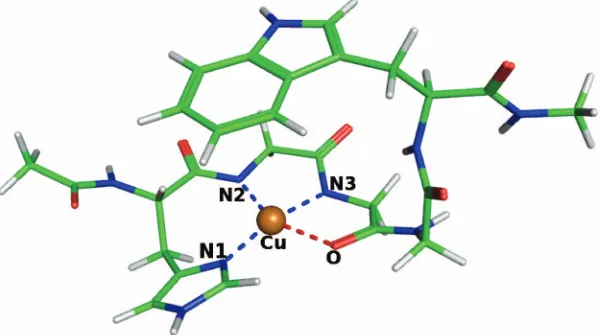
number of atoms in the fragment is 72. The protein fragment is first molded into a shape resembling the binding side ge-ometry obtained from experiment.75The system is then sol-vated with 3101 water molecules. The KS electron and the full simulation cells are cubic with sides of 22.49 and 44.98 Å, respectively. The water molecules closer to the cop-per ion than 6 Å are treated by KS DFT, which typically adds 12 water molecules to the KS subsystem, increasing the total number of KS atoms to 108. This system is equilibrated by first running molecular dynamics at 300 K for FDOF molecules only for 5000 steps, with the KS part frozen, and then 750 steps of molecular dynamics is performed for the entire system. Following the simulation, the structure of the hybrid system was relaxed. The resulting structure is shown in Fig. 5.
The calculated binding site geometry is quite similar to that obtained in Ref. 78. The Cu–N bonds differ only by a few hundreds of angstroms, while the Cu–O bond is 2.35 Å instead of 2.09 Å. A significant part of this difference ap-pears to be due to the different treatment of the solvent in Ref.78, where only the first solvation shell was explicit and
the rest of the solvent was modeled implicitly. In our calcu-lation, two water molecules are found in contact with the copper ion, which are stabilized by hydrogen bonding with other water molecules present in the system. No water mol-ecules close to the copper are reported in Ref.78. The pres-ence of these two water molecules is the major cause of the difference between the two calculations: When the calcula-tion is performed without the water molecules in contact with copper, the difference in Cu–O bond distance decreases by more than half to only 0.11 Å, while other bonds involv-ing copper stay almost unchanged.
The binding energy of the copper ion to the PrP was also calculated. To obtain it, the energy of a free protein fragment with protonated backbone nitrogens 共EfragH
2兲
was calculated when solvated with the same number of water molecules as the copper-bound fragment. We also computed the energy of a copper atom共ECu兲and the energy of a hydrogen molecule
H2 共EH2兲. The copper ion binding energy can then be
ob-tained as
Ebind
Cu=EfragCu−EfragH2−ECu+EH2, 共19兲
where Efrag
Cu is the energy of the relaxed solvated
HGGGW–Cu complex shown in Fig. 5. By calculating all four energies, we obtain 1.76 eV as the binding energy of the copper ion. We are not aware of any calculated or measured binding energy of copper ions in biological systems, but our calculated value is similar to the binding energy of a copper atom in copper clusters Cu4 and Cu13 共1.26 and 2.19 eV
respectively兲.80
Additional calculations on copper binding to the PrP are in progress, which address different copper binding modes and the resulting structural changes in the protein. The re-sults of these calculations will be reported elsewhere.
VIII. SUMMARY AND CONCLUSIONS
In simulations involving proteins or other biomolecules, the solvent plays an important role and its effects cannot be neglected. In a typical protein simulation, the number of at-oms in the solvent is by far greater than the number of atat-oms in the solvated protein. The hybrid method presented in this paper is designed for such biosimulations. The biomolecule, or its fragment, and solvent molecules in the first solvation shells are treated by full Kohn-Sham DFT, while the remain-ing solvent molecules are efficiently described usremain-ing a frozen-density orbital-free DFT. We have shown that this ap-proach allows for an efficient and accurate description of the solvent effects and that it provides seamless integration be-tween the regions treated by different DFT methods.
At present, the hybrid method requires that the biomol-ecules are fully treated by the KS DFT, which means that it can only treat biomolecular fragments with no more than a few hundred atoms. Hybrid simulations for large biomol-ecules with the current method are possible but require de-veloping of charge density parametrization for important parts of biomolecules, such as amino acids in the case of proteins.
In the near future, the need for treating biomolecules by two different methods may decrease due to the steady
ad-vances in computer power and computational methods. Cur-rent state-of-the-art supercomputers contain tens of thou-sands of processors and this number is expected to increase rapidly over the next few years. This will allow quantum calculations on systems with thousands of atoms especially when linear-scaling methods are used. When such calcula-tions become feasible, the present hybrid method will allow for simulation of fully solvated, full-length biomolecules at the quantum level, which at present can only be performed using classical potentials.
ACKNOWLEDGMENTS
We gratefully acknowledge support by NSF, DOE, DOD, and ORNL-LDRD and grants of supercomputer time provided by DOE and the DOD Challenge Program.
1P. Hohenberg and W. Kohn, Phys. Rev. 136, B864共1964兲.
2W. Kohn and L. J. Sham, Phys. Rev. 140, A1133共1965兲.
3J. Tomasi and M. Persico, Chem. Rev.共Washington, D.C.兲 94, 2027
共1994兲.
4J. L. Rivail and D. Rinald,Liquid State Quantum Chemistry:
Computa-tional Applications of The Polarizable Continuum Models共World Scien-tific, Singapore, 1995兲.
5C. J. Cramer and D. G. Truhlar,Continuum Solvation Models共Kluwer, Dordrecht, 1996兲.
6J. Fattebert and F. Gygi, J. Comput. Chem. 23, 662共2002兲.
7D. Begue, P. Carbonniere, V. Barone, and C. Pouchan, Chem. Phys. Lett.
416, 206共2005兲.
8L. Guimarães, H. Avelino de Abreu, and H. Duarte, Chem. Phys.333, 10
共2007兲.
9P. Bonifassi, P. Ray, and J. Leszczynski, Chem. Phys. Lett. 431, 321
共2006兲.
10R. Zhou and B. Berne, Proc. Natl. Acad. Sci. U.S.A. 99, 12777共2002兲.
11Y. M. Rhee, E. J. Sorin, G. Jayachandran, E. Lindahl, and V. S. Pande,
Proc. Natl. Acad. Sci. U.S.A. 101, 6456共2004兲.
12S. Miertus, E. Scrocco, and J. Tomasi, Chem. Phys. 55, 117共1981兲.
13R. Cammi and J. Tomasi, J. Comput. Chem. 16, 1449共1995兲.
14A. Warshel and M. Levitt, J. Mol. Biol. 102, 227共1976兲.
15U. C. Singh and P. A. Kollmann, J. Comput. Chem. 7, 718共1986兲.
16M. J. Field, P. A. Bash, and M. Karplus, J. Comput. Chem. 11, 700
共1990兲.
17T. Kerdcharoen and K. Morokuma, Chem. Phys. Lett. 355, 257共2002兲.
18L. Thomas, Proc. Cambridge Philos. Soc. 23, 542共1927兲.
19E. Fermi, Rend. Accad. Naz. Lincei 6, 602共1927兲.
20E. Fermi, Z. Phys. 48, 73共1928兲.
21C. von Weizsacker, Z. Phys. 96, 431共1934兲.
22R. O. Jones and O. Gunnarsson, Rev. Mod. Phys. 61, 689共1989兲.
23Y. Wang and E. Carter,Orbital Free Kinetic Energy Density Functional
Theory共Kluwer, Dordrecht, 2000兲, Chap. 5, pp. 117–184. 24A. E. DePristo and J. D. Kress, Phys. Rev. A 35, 438共1987兲.
25A. J. Thakkar, Phys. Rev. A 46, 6920共1992兲.
26P. I. Plindov and S. K. Pogrebnya, Chem. Phys. Lett. 143, 535共1988兲.
27J. P. Perdew, Phys. Lett. A 165, 79共1992兲.
28H. Lee, C. Lee, and R. Parr, Phys. Rev. A 44, 768共1991兲.
29D. Lacks and R. Gordon, J. Chem. Phys. 100, 4446共1994兲.
30A. D. Becke, Phys. Rev. A 38, 3098共1988兲.
31J. A. Alonso and L. A. Girifalco, Phys. Rev. B 17, 3735共1978兲.
32E. Chacón, J. E. Alvarellos, and P. Tarazona, Phys. Rev. B 32, 7868
共1985兲.
33E. Smargiassi and P. A. Madden, Phys. Rev. B 49, 5220共1994兲.
34Y. A. Wang, N. Govind, and E. A. Carter, Phys. Rev. B 58, 13465
共1998兲.
35Y. A. Wang, N. Govind, and E. A. Carter, Phys. Rev. B 60, 16350
共1999兲.
36R. Gordon and Y. Kim, J. Chem. Phys. 61, 3122共1972兲.
37Y. Kim and R. Gordon, Phys. Rev. B 9, 3548共1974兲.
38T. Wesolowski and A. Warshel, J. Phys.: Condens. Matter 97, 8050
共1993兲.
39T. Wesolowski and A. Warshel, J. Phys.: Condens. Matter 98, 5183
40D. Barker and M. Sprik, Mol. Phys. 101, 1183共2003兲.
41P. Huang and E. A. Carter, J. Chem. Phys. 125, 084102共2006兲.
42D. R. Hamann, M. Schlüter, and C. Chiang, Phys. Rev. Lett. 43, 1494
共1979兲.
43G. P. Kerker, J. Phys. C 13, L189共1980兲.
44A. Zunger and M. L. Cohen, Phys. Rev. B 18, 5449共1978兲.
45L. Kleinman and D. M. Bylander, Phys. Rev. Lett. 48, 1425共1982兲.
46D. Vanderbilt, Phys. Rev. B 41, 7892共1990兲.
47T. Starkloff and J. D. Joannopoulos, Phys. Rev. B 16, 5212共1977兲.
48S. C. Watson, B. J. Jesson, E. A. Carter, and P. A. Madden, Europhys.
Lett. 41, 37共1998兲.
49V. Shah, D. Nehete, and D. G. Kanhere, Z. Phys. 48, 73共1928兲.
50D. Nehete, V. Shah, and D. G. Kanhere, Phys. Rev. B 53, 2126共1996兲.
51A. Dhavale, V. Shah, and D. G. Kanhere, Phys. Rev. A 57, 4522共1998兲.
52E. L. Briggs, D. J. Sullivan, and J. Bernholc, Phys. Rev. B 52, 5471
共1995兲.
53E. L. Briggs, D. J. Sullivan, and J. Bernholc, Phys. Rev. B 54, 14362
共1996兲.
54M. Hodak, S. Wang, W. Lu, and J. Bernholc, Phys. Rev. B 76, 085108
共2007兲.
55J. Ryckaert, G. Ciccotti, and H. Berendsen, J. Comp. Phys. 23, 327
共1977兲.
56P. L. Silvestrelli and M. Parrinello, J. Chem. Phys. 111, 3572共1999兲.
57A. Shepard, G. Beers, G. Klein, and L. Rothmann, J. Chem. Phys. 59,
2254共1973兲.
58C. Coulson and D. Eisenbero, Proc. R. Soc. London, Ser. A 291, 445
共1966兲.
59E. Batista, S. Xantheas, and H. Jonsson, J. Chem. Phys. 109, 4546
共1998兲.
60M. Heggie, C. L. Latham, and S. Maynard, and R. Jones, Chem. Phys.
Lett. 249, 485共1996兲.
61Y. Badyal, M. Saboungi, D. Price, S. Shastri, D. Haeffner, and A. Soper,
J. Chem. Phys. 112, 9206共2000兲.
62P. L. Silvestrelli and M. Parrinello, Phys. Rev. Lett. 82, 3308共1999兲.
63A. K. Soper, Chem. Phys. 258, 121共2000兲.
64J. P. Perdew, K. Burke, and M. Ernzerhof, Phys. Rev. Lett. 77, 3865
共1996兲.
65J. P. Perdew, K. Burke, and M. Ernzerhof, Phys. Rev. Lett. 78, 1396
共1997兲.
66J. Grossman, E. Schwegler, E. Draeger, F. Gygi, and G. Galli, J. Chem.
Phys. 120, 300共2004兲.
67E. Schwegler, J. Grossman, F. Gygi, and G. Galli, J. Chem. Phys. 121,
5400共2004兲.
68M. Sprik, J. Hutter, and M. Parrinello, J. Chem. Phys. 105, 1142共1996兲.
69T. Wesolowski, R. Muller, and A. Warshel, J. Phys.: Condens. Matter
100, 15444共1996兲.
70T. Wesolowski and J. Weber, Chem. Phys. Lett. 248, 71共1996兲.
71S. Prusiner, Science 278, 245共1997兲.
72N. Vassallo and J. Herms, J. Neurochem. 86, 538共2003兲.
73N. Inestrosa, W. Cerpa, and L. Varela-Nallar, IUBMB Life 57, 645
共2005兲.
74D. Brown, K. Qin, J. Herms, A. Madlung, J. Manson, R. Strome, P.
Fraser, T. Kruck, A. von Bohlen, W. Schulz-Schaeffer, A. Giese, D. Westaway, and H. Kretzschmar, Nature共London兲 390, 684共1997兲. 75G. Millhauser, Acc. Chem. Res. 37, 79共2004兲.
76R. Whittal, H. Ball, F. Cohen, A. Prusiner, and M. Baldwin, Protein Sci.
9, 332共2000兲.
77P. Pauly and D. Harris, J. Biol. Chem. 273, 33107共1998兲.
78M. Pushie and A. Rauk, JBIC, J. Biol. Inorg. Chem. 8, 53共2003兲.
79H.-F. Ji and H.-Y. Zhang, Chem. Res. Toxicol. 17, 471共2004兲.
80B. Delley, D. E. Ellis, A. J. Freeman, E. J. Baerends, and D. Post, Phys.